Closed-Form Solution of the Bending Two-Phase Integral Model of Euler-Bernoulli Nanobeams

Abstract

Recent developments have shown that the widely used simplified differential model of Eringen’s nonlocal elasticity in nanobeam analysis is not equivalent to the corresponding and initially proposed integral models, the pure integral model and the two-phase integral model, in all cases of loading and boundary conditions. This has resolved a paradox with solutions that are not in line with the expected softening effect of the nonlocal theory that appears in all other cases. In addition, it revived interest in the integral model and the two-phase integral model, which were not used due to their complexity in solving the relevant integral and integro-differential equations, respectively. In this article, we use a direct operator method for solving boundary value problems for nth order linear Volterra–Fredholm integro-differential equations of convolution type to construct closed-form solutions to the two-phase integral model of Euler–Bernoulli nanobeams in bending under transverse distributed load and various types of boundary conditions.

1. Introduction

The classical or local theory of elasticity is scale-free. As a result, it cannot cope with situations where an internal characteristic length of material becomes comparable to an external geometric length. This is the case with micro- and nano-scale structures [1]. A remedy for these situations is the use of generalized continuity theories such as the higher-order continuum theories, namely the Cosserat theory [2], the couple stress theory [3], the micropolar theory [4], the strain gradient theory [5,6,7], and the nonlocal theories [8,9,10]. They incorporate additional material parameters in the constitutive equations that increase the complexity, and therefore, numerical methods, such as the finite element method, are employed to solve the governing equations, see for example in [11,12,13,14,15,16,17]. For similar developments in the field of thermoelasticity, one can see the very recent publications [18,19,20].

In the nonlocal continuum theory of elasticity developed by Eringen [10], the stress state at a point does not depend only on the strain at that particular point as in classical elasticity (local model) but is defined as an integrated average of the strain field at every point in the body (integral model). A variant of this integral model is the two-phase integral model (integro-differential model) that combines the local model and the nonlocal integral model [21,22,23]. Both integral models are associated with governing equations involving integral or integro-differential equations that are difficult to solve. A simplified form of nonlocality is the differential model, which includes a degenerated differential form of the integral model [10].

Due to its simplicity, the nonlocal differential model has widely been used to analyze various micro- and nano-structures including one-dimensional structures such as rods, tubes, and beams [24,25,26]. In particular, for the beam bending analysis, the interested reader can look at, among others, [27,28,29,30,31]. However, several authors have reported that the nonlocal differential model for certain types of loading gives inconsistent results compared to those obtained from other types of loading and boundary conditions [27,32]. This paradox was recently explained in [33] where it is shown that, in general, the nonlocal differential model is not equivalent to its integral counterpart unless certain conditions are met, as defined in [34].

This development has revived the interest in the nonlocal integral models, and therefore, there is a need to develop effective methods for producing exact analytical solutions. A closed-form solution of the nonlocal integral model for the bending of Euler–Bernoulli beams was recently obtained in [35]. Moreover, an analytical solution for the two-phase nonlocal integral model was obtained in [36] through a reduction to a differential equation with mixed boundary conditions as proposed by [34]. In general, integro-differential equations are usually difficult to solve directly. In the last few years, the authors have developed a direct operator technique for solving exactly Fredholm-type integro-differential equations (FIDE) with all kinds of boundary conditions, including nonlocal ones [37,38]. In [39], a method for solving in closed form boundary value problems for a class of nth order linear Volterra–Fredholm integro-differential equations (VFIDE) of convolution type was proposed. The technique was used to construct the closed-form solution of the boundary value problem for the two-phase nonlocal integral model of Euler–Bernoulli beams under a uniformly transverse distributed load and in the case of simply supported boundary conditions. In this article, we provide the closed-form solution for three more boundary value problems corresponding to three practical cases of boundary conditions, specifically a cantilever beam, a clamped pinned beam, and a clamped beam. Exact analytical solutions to these three boundary value problems through a direct operator method for integro-differential equations do not exist in the literature.

The outline of the article is as follows. In Section 2, the notation is explained, and the direct procedure for solving exactly Volterra–Fredholm integro-differential boundary value problems of convolution type is recalled. In Section 3, the closed-form solution of the integro-differential bending model of Euler–Bernoulli beams for three different types of boundary conditions are obtained, and an algorithm for their calculation in a computer algebra system is provided. Examples and discussion are given in Section 4. Finally, some conclusions are presented in Section 5.

2. Closed-Form Solution of Volterra–Fredholm Integro-Differential Equations

Let $X=C[0,L]$, $L\in {\mathbb{R}}^{+}$, and $A:X\to X$ be an nth order linear differential operator of the form

$$Au=\sum _{i=0}^n{a}_i{u}^{(n-i)}\left(x\right),\mathcal{D}\left(A\right)=\{u\in X_n:\mathrm{\Phi }\left(u\right)=\mathbf{0}\},$$

(1)

where $n\in \mathbb{N}$, $a_i,i=0,1,\dots ,n,$ are real constants with $a_0\ne 0$, $X_n=C^n[0,L],X_0=X$, $u=u\left(x\right)\in X_n$, $u^{\left(i\right)}\left(x\right)=\frac{d^{i}u}{d{x}^i},i=1,2,\dots ,n,$

$$\mathrm{\Phi }\left(u\right)=\left(\begin{array}{c}{\mathrm{\Phi }}_1\left(u\right)\\ {\mathrm{\Phi }}_2\left(u\right)\\ ⋮\\ {\mathrm{\Phi }}_n\left(u\right)\end{array}\right),\mathrm{\Phi }\in {\left[X_{n-1}^{*}\right]}^n,{\mathrm{\Phi }}_i\in X_{n-1}^{*},i=1,2,\dots ,n,$$

(2)

is a column vector of linear functionals that describe the specified boundary conditions, and 0 denotes the zero column vector.

Let $K:X\to X$ be the linear Volterra integral operator of convolution type

$$Ku=\sum _{i=0}^n{\int }_0^x{k}_i(x-t)u^{(n-i)}\left(t\right)dt,$$

(3)

where the kernels $k_i\left(x\right)\in X,i=0,1,\dots ,n$.

Let the Fredholm-type functionals

$${\int }_0^L{\overline{k}}_j(x,t)Au\left(t\right)dt,j=1,2,\dots ,m,$$

(4)

where the kernels ${\overline{k}}_j(x,t)\in X\times X$ are assumed to be separable, i.e.,

$${\overline{k}}_j(x,t)=g_j\left(x\right)h_j\left(t\right),g_j=g_j\left(x\right),h_j=h_j\left(t\right)\in X,j=1,2,\dots ,m.$$

(5)

Let the row vector of functions

$$g=\left(\begin{array}{cccc}{g}_1& g_2& \cdots & g_m\end{array}\right),g\in X^m,$$

(6)

and the column vector of functionals

$$\mathrm{\Psi }\left(Au\right)=\left(\begin{array}{c}{\mathrm{\Psi }}_1\left(Au\right)\\ {\mathrm{\Psi }}_2\left(Au\right)\\ ⋮\\ {\mathrm{\Psi }}_m\left(Au\right)\end{array}\right),{\mathrm{\Psi }}_j\left(Au\right)={\int }_0^L{h}_j\left(t\right)Au\left(t\right)dt,j=1,2,\dots ,m,$$

(7)

where $\mathrm{\Psi }\in {\left[X^{*}\right]}^m$ and ${\mathrm{\Psi }}_j\in X^{*},j=1,2,\dots ,m$.

Consider the linear Volterra–Fredholm type integro-differential operator $T:X\to X$ defined by

$$\begin{array}{ccc}\hfill Tu& =& Au+Ku-\sum _{j=1}^m{g}_j{\mathrm{\Psi }}_j\left(Au\right)=Au+Ku-g\mathrm{\Psi }\left(Au\right),\hfill \\ \hfill \mathcal{D}\left(T\right)& =& \mathcal{D}\left(A\right)=\{u\in X_n:\mathrm{\Phi }\left(u\right)=\mathbf{0}\},\hfill \end{array}$$

(8)

and the Volterra–Fredholm integro-differential boundary value problem

$$\begin{array}{c}\hfill VFIDBVP:Tu=f,f=f\left(x\right)\in X.\end{array}$$

(9)

Let the $m\times m$ matrix

$$\mathrm{\Psi }\left(g\right)=\left(\begin{array}{cccc}{\mathrm{\Psi }}_1\left(g_1\right)& {\mathrm{\Psi }}_1\left(g_2\right)& \cdots & {\mathrm{\Psi }}_1\left(g_m\right)\\ {\mathrm{\Psi }}_2\left(g_1\right)& {\mathrm{\Psi }}_2\left(g_2\right)& \cdots & {\mathrm{\Psi }}_2\left(g_m\right)\\ ⋮& ⋮& \ddots & ⋮\\ {\mathrm{\Psi }}_m\left(g_1\right)& {\mathrm{\Psi }}_m\left(g_2\right)& \cdots & {\mathrm{\Psi }}_m\left(g_m\right)\end{array}\right),$$

where the element ${\mathrm{\Psi }}_i\left(g_j\right)$ is the value of the functional ${\mathrm{\Psi }}_i$ on the element $g_j$, and $I_m$ denotes the $m\times m$ identity matrix.

The criteria for the existence of a unique solution of the VFIDBVP in (9) and a formula for its symbolic calculation in an exact closed form are given in [39] where the following theorem has been proved.

Theorem 1.

Let the operator $T:X\to X$ be defined as in (8). Assume that the Volterra integro-differential operator $D:X\to X$ defined by

$$Du=(A+K)u,\mathcal{D}\left(D\right)=\mathcal{D}\left(A\right),$$

(10)

is bijective on X and its inverse is denoted by $D^{-1}={(A+K)}^{-1}$. Then, the operator T is bijective, precisely it is injective if and only if

$$detW=det\left[I_m-\mathrm{\Psi }\left(A{D}^{-1}g\right)\right]\ne 0,$$

(11)

and in this case, the unique solution to the boundary value problem

$$Tu=f,\mathrm{for}\mathrm{all}\mathrm{functions}f\in X,$$

(12)

is given by the formula

$$\begin{array}{ccc}\hfill u& =& T^{-1}f\hfill \\ & =& D^{-1}f+D^{-1}g{W}^{-1}\mathrm{\Psi }\left(A{D}^{-1}f\right).\hfill \end{array}$$

(13)

3. Closed-Form Solution of Eringen’s Two-Phase Integral Model Equations

In a right-handed coordinate system, consider a uniform beam of length L and cross-sectional area S whose longitudinal axis coincides with the x-axis and with one end at $x=0$ and the other at $x=L$. The beam is loaded by a transverse distributed load $q\left(x\right)$ at the top in the z-direction.

Under the Euler–Bernoulli assumptions and for a homogeneous and isotropic material, the transverse displacement in the z-direction (deflection) $w\left(x\right)$ is a function of x, and the strain in the x-direction is defined by

$${\epsilon }_x\left(x\right)=-z\frac{d^{2}w\left(x\right)}{d{x}^2}$$

In the two-phase nonlocal Eringen’s elasticity model, the stress ${\sigma }_x\left(x\right)$ is defined through the constitutive relation

$${\sigma }_x\left(x\right)=E\left({\xi }_1{\epsilon }_x\left(x\right)+{\xi }_2{\int }_0^{L}k(x,t){\epsilon }_x\left(t\right)dt\right),$$

and the corresponding bending moment is defined by

$$M\left(x\right)={\int }_S^{}{\sigma }_x\left(x\right)zdS=-EI\left({\xi }_1\frac{d^{2}w\left(x\right)}{d{x}^2}+{\xi }_2{\int }_0^{L}k(x,t)\frac{d^{2}w\left(t\right)}{d{t}^2}dt\right),$$

(14)

where E is the elasticity modulus (constant) and $I={\int }_S^{}{z}^{2}dS$ is the second moment of area. The parameters ${\xi }_1>0$, ${\xi }_2>0$ and ${\xi }_1+{\xi }_2=1$ regulate the contribution from the local (classical) and nonlocal model, respectively. The kernel or attenuation function $k(x,t)$ determines the nonlocal effect of the strain ${\epsilon }_x\left(t\right)$ at the source point t on the stress ${\sigma }_x\left(x\right)$ at the receiver point x. There are many possible kernel functions $k(x,t)$. The most commonly used is the Helmholtz-type kernel

$$k(x,t)=\frac{1}{2\tau }{e}^{-\frac{|x-t|}{\tau }},x,t\in [0,L],$$

(15)

where the parameter $\tau =\frac{e_{0}a}{\ell }$, $e_0$ is a material constant, a is an internal characteristic length (e.g., lattice parameter, granular distance), and ℓ is an external characteristic length (e.g., the crack length, the wave length). The kernel $k(x,t)$ is a positive function which diminishes rapidly as $|x-t|$ increases and satisfies the normalizing condition ${\int }_0^{L}k(x,t)dt=1$.

The equilibrium equation in terms of the displacement $w\left(x\right)$ is

$$-EI\frac{d^2}{d{x}^2}\left({\xi }_1\frac{d^{2}w\left(x\right)}{d{x}^2}+{\xi }_2{\int }_0^{L}k(x,t)\frac{d^{2}w\left(t\right)}{d{t}^2}dt\right)+q\left(x\right)=0,0<x<L,$$

(16)

and the boundary conditions

$$w\left(x\right)or{M}^{\prime }\left(x\right),$$

(17)

and

$$w^{\prime }\left(x\right)orM\left(x\right),$$

(18)

specified at each of the two ends of the beam at $x=0$ and $x=L$.

Next, we look at the four most common cases of boundary conditions with practical interest. In each case, we formulate the corresponding boundary value problem in operator form and decomposed it in two lower-order problems, namely a second-order differential boundary value problem (DBVP) and a second-order Fredholm integro-differential boundary value problem (FIDBVP). The solution is obtained by first solving the DBVP in closed form and then the FIDBVP.

For convolution kernels of the type (15), the FIDBVP is converted to a Volterra–Fredholm integro-differential boundary value problem (VFIDBVP), which is then solved by using Theorem 1.

3.1. Simply Supported Beam (SS)

For a beam simply supported at both ends, the boundary conditions imposed at $x=0$ and $x=L$ are

$$w\left(0\right)=w\left(L\right)=0,M\left(0\right)=M\left(L\right)=0.$$

(19)

This problem is solved in detail in [39] and is not discussed further here.

3.2. Cantilever Beam (CF)

Let us consider the case of a cantilever beam subject to the following boundary conditions

$$w\left(0\right)=w^{\prime }\left(0\right)=0,M\left(L\right)=M^{\prime }\left(L\right)=0.$$

(20)

Let $X=C[0,L]$. Taking into account the equilibrium Equation (16) and the definition (14), we define the operator $B:X\to X$ as

$$\begin{array}{ccc}\hfill Bw\left(x\right)& =& \frac{d^2}{d{x}^2}\left(\frac{d^{2}w\left(x\right)}{d{x}^2}+\frac{{\xi }_2}{{\xi }_1}{\int }_0^{L}k(x,t)\frac{d^{2}w\left(t\right)}{d{t}^2}dt\right),\hfill \\ \hfill \mathcal{D}\left(B\right)& =& \left\{w\left(x\right)\in C^4[0,L]:w\left(0\right)=w^{\prime }\left(0\right)=0,\right.\hfill \\ & & {\left[\frac{d^{2}w\left(x\right)}{d{x}^2}+\frac{{\xi }_2}{{\xi }_1}{\int }_0^{x}k(x,t)\frac{d^{2}w\left(t\right)}{d{t}^2}dt\right]}_{x=L}=0,\hfill \\ & & \left.{\left[\frac{d}{dx}\left(\frac{d^{2}w\left(x\right)}{d{x}^2}+\frac{{\xi }_2}{{\xi }_1}{\int }_0^{x}k(x,t)\frac{d^{2}w\left(t\right)}{d{t}^2}dt\right)\right]}_{x=L}=0\right\},\hfill \end{array}$$

and write the boundary value problem (16), (20) in the compact form

$$Bw\left(x\right)=\frac{1}{EI{\xi }_1}q\left(x\right),0<x<L,q\left(x\right)\in X.$$

(21)

Let the Fredholm integro-differential operator $B_2:X\to X$ be defined by

$$\begin{array}{ccc}\hfill B_{2}w\left(x\right)& =& \frac{d^{2}w\left(x\right)}{d{x}^2}+\frac{{\xi }_2}{{\xi }_1}{\int }_0^{L}k(x,t)\frac{d^{2}w\left(t\right)}{d{t}^2}dt,\hfill \\ \hfill \mathcal{D}\left(B_2\right)& =& \left\{w\left(x\right)\in C^2[0,L]:w\left(0\right)=w^{\prime }\left(0\right)=0\right\}.\hfill \end{array}$$

(22)

Furthermore, let the differential operator $B_1:X\to X$ be

$$\begin{array}{ccc}\hfill B_{1}y\left(x\right)& =& \frac{d^{2}y\left(x\right)}{d{x}^2},\hfill \\ \hfill \mathcal{D}\left(B_1\right)& =& \left\{y\left(x\right)\in C^2[0,L]:y\left(L\right)=y^{\prime }\left(L\right)=0\right\}.\hfill \end{array}$$

If we take $y\left(x\right)=B_{2}w\left(x\right)$, then

$$\begin{array}{ccc}\hfill \mathcal{D}\left(B_1{B}_2\right)& =& \left\{w\left(x\right)\in C^2[0,L]:w\left(0\right)=w^{\prime }\left(0\right)=0,y\left(x\right)=B_{2}w\left(x\right)\in D\left(B_1\right)\right\}\hfill \\ & =& \left\{w\left(x\right)\in C^2[0,L]:w\left(0\right)=w^{\prime }\left(0\right)=0,y\left(x\right)\in C^2[0,L],y\left(L\right)=y^{\prime }\left(L\right)=0\right\}\hfill \\ & =& \left\{w\left(x\right)\in C^4[0,L]:w\left(0\right)=w^{\prime }\left(0\right)=0,\right.\hfill \\ & & {\left[\frac{d^{2}w\left(x\right)}{d{x}^2}+\frac{{\xi }_2}{{\xi }_1}{\int }_0^{x}k(x,t)\frac{d^{2}w\left(t\right)}{d{t}^2}dt\right]}_{x=L}=0,\hfill \\ & & \left.{\left[\frac{d}{dx}\left(\frac{d^{2}w\left(x\right)}{d{x}^2}+\frac{{\xi }_2}{{\xi }_1}{\int }_0^{x}k(x,t)\frac{d^{2}w\left(t\right)}{d{t}^2}dt\right)\right]}_{x=L}=0\right\}\hfill \\ & =& \mathcal{D}\left(B\right).\hfill \end{array}$$

That is, the operator B can be factorized as $B=B_1{B}_2$, and therefore, the boundary value problem (21) is carried to

$$B_1{B}_{2}w\left(x\right)=\frac{1}{EI{\xi }_1}q\left(x\right),0<x<L,q\left(x\right)\in X.$$

(23)

The solution of (23) can now be obtained by solving the following two boundary value problems, namely the differential boundary value problem

$$\mathrm{DBVP}:B_{1}y\left(x\right)=\frac{1}{EI{\xi }_1}q\left(x\right),0<x<L,q\left(x\right)\in X,$$

(24)

and the Fredholm integro-differential boundary value problem

$$\begin{array}{c}\hfill \mathrm{FIDBVP}:B_{2}w\left(x\right)=y\left(x\right),0<x<L.\end{array}$$

(25)

The solution of DBVP in (24) in closed form for any $q\left(x\right)\in X$ is given by

$$\begin{array}{ccc}\hfill y\left(x\right)& =& B_1^{-1}\left(\frac{1}{EI{\xi }_1}q\left(x\right)\right)\hfill \\ & =& \frac{1}{EI{\xi }_1}\left[{\int }_0^x(x-t)q\left(t\right)dt-x{\int }_0^{L}q\left(t\right)dt+{\int }_0^{L}tq\left(t\right)dt\right],\hfill \end{array}$$

(26)

see, for example, in [40].

The solution procedure for the FIDBVP in (25) is determined by the type of the kernel $k(x,t)$. For a kernel function of the type (15), the operator $B_2$ in (22) by removing the modulus in the integrand can be written equivalently as the Volterra–Fredholm integro-differential operator

$$\begin{array}{ccc}\hfill B_{2}w\left(x\right)& =& \frac{d^{2}w\left(x\right)}{d{x}^2}-\frac{{\xi }_2}{\tau {\xi }_1}{\int }_0^{x}sinh\left(\frac{x-t}{\tau }\right)\frac{d^{2}w\left(t\right)}{d{t}^2}dt+\frac{{\xi }_2}{2\tau {\xi }_1}{e}^{\frac{x}{\tau }}{\int }_0^L{e}^{-\frac{t}{\tau }}\frac{d^{2}w\left(t\right)}{d{t}^2}dt,\hfill \\ \hfill \mathcal{D}\left(B_2\right)& =& \left\{w\left(x\right)\in C^2[0,L]:w\left(0\right)=w^{\prime }\left(0\right)=0\right\},\hfill \end{array}$$

(27)

see [39] for details, and as a result, the FIDBVP in (25) degenerates to the Volterra–Fredholm integro-differential boundary value problem

$$\begin{array}{c}\hfill \mathrm{VFIDBVP}:B_{2}w\left(x\right)=y\left(x\right),0<x<L.\end{array}$$

(28)

After substituting (26) into (28), the exact solution of VFIDBVP can be obtained by applying Theorem 1. Comparing (28) with (9), we take $n=2$, $m=1$,

$$\begin{array}{ccc}\hfill Aw\left(x\right)& =& \frac{d^{2}w\left(x\right)}{d{x}^2},\mathcal{D}\left(A\right)=\{w\left(x\right)\in C^2[0,L]:\mathrm{\Phi }\left(w\right)=\mathbf{0}\},\hfill \\ \hfill \mathrm{\Phi }\left(w\right)& =& \left(\begin{array}{c}{\mathrm{\Phi }}_1\left(w\right)\\ {\mathrm{\Phi }}_2\left(w\right)\end{array}\right)=\left(\begin{array}{c}w\left(0\right)\\ w^{\prime }\left(0\right)\end{array}\right),\hfill \\ \hfill Kw\left(x\right)& =& -\frac{{\xi }_2}{\tau {\xi }_1}{\int }_0^{x}sinh\left(\frac{x-t}{\tau }\right)\frac{d^{2}w\left(t\right)}{d{t}^2}dt,\hfill \\ \hfill g\left(x\right)& =& \left(-\frac{{\xi }_2}{2\tau {\xi }_1}{e}^{\frac{x}{\tau }}\right),\hfill \\ \hfill \mathrm{\Psi }\left(Aw\right)& =& \left({\int }_0^L{e}^{-\frac{t}{\tau }}\frac{d^{2}w\left(t\right)}{d{t}^2}dt\right),\hfill \\ \hfill f\left(x\right)& =& \frac{1}{EI{\xi }_1}\left[{\int }_0^x(x-t)q\left(t\right)dt-x{\int }_0^{L}q\left(t\right)dt+{\int }_0^{L}tq\left(t\right)dt\right].\hfill \end{array}$$

In addition, we have

$$\begin{array}{ccc}\hfill Dz\left(x\right)& =& (A+K)z\left(x\right)=\frac{d^{2}z\left(x\right)}{d{x}^2}-\frac{{\xi }_2}{\tau {\xi }_1}{\int }_0^{x}sinh\left(\frac{x-t}{\tau }\right)\frac{d^{2}z\left(t\right)}{d{t}^2}dt,\hfill \\ \hfill \mathcal{D}\left(D\right)& =& \mathcal{D}\left(A\right)=\{z\left(x\right)\in C^2[0,L]:\mathrm{\Phi }\left(z\right)=\mathbf{0}\}.\hfill \end{array}$$

First, we find the inverse operator $D^{-1}$ by solving the boundary value problem $Dz\left(x\right)=f\left(x\right)$ via the Laplace transform method. By applying the Laplace transform operator on both sides, using the convolution theorem and utilizing the boundary conditions $z\left(x\right)=z^{\prime }\left(x\right)=0$, we get

$$\begin{array}{ccc}\hfill \mathcal{L}\left\{Dz\left(x\right)\right\}& =& \mathcal{L}\left\{\frac{d^{2}z\left(x\right)}{d{x}^2}\right\}-\frac{{\xi }_2}{\tau {\xi }_1}\mathcal{L}\left\{sinh\left(\frac{x}{\tau }\right)\right\}\mathcal{L}\left\{\frac{d^{2}z\left(x\right)}{d{x}^2}\right\}\hfill \\ & =& \left[1-\frac{{\xi }_2}{\tau {\xi }_1}\left(\frac{\frac{1}{\tau }}{s^2-\frac{1}{{\tau }^2}}\right)\right]s^{2}Z\left(s\right)=F\left(s\right),\hfill \end{array}$$

from where it follows that

$$Z\left(s\right)=F\left(s\right)Q\left(s\right),$$

(29)

where

$$Z\left(s\right)=\mathcal{L}\left\{z\left(x\right)\right\},F\left(s\right)=\mathcal{L}\left\{f\left(x\right)\right\},Q\left(s\right)=\frac{{\xi }_1({\tau }^2{s}^2-1)}{s^2({\xi }_1{\tau }^2{s}^2-1)}.$$

Taking the inverse Laplace transform of (29), we obtain

$$z\left(x\right)=D^{-1}f\left(x\right)={\mathcal{L}}^{-1}\left\{F\left(s\right)Q\left(s\right)\right\}.$$

(30)

Since Equation (30) holds for every $f\left(x\right)\in X$, it is implied that the operator D is bijective.

Next, we compute

$$D^{-1}g\left(x\right)=D^{-1}\left(-\frac{{\xi }_2}{2\tau {\xi }_1}{e}^{\frac{x}{\tau }}\right)={\mathcal{L}}^{-1}\left\{G\left(s\right)Q\left(s\right)\right\},$$

(31)

where $G\left(s\right)=\mathcal{L}\left\{g\left(x\right)\right\}$, and subsequently

$$\begin{array}{ccc}\hfill A{D}^{-1}g\left(x\right)& =& \frac{d^2}{d{x}^2}\left(D^{-1}g\left(x\right)\right),\hfill \\ \hfill \mathrm{\Psi }\left(A{D}^{-1}g\left(x\right)\right)& =& {\int }_0^L{e}^{-\frac{t}{\tau }}A{D}^{-1}g\left(t\right)dt.\hfill \end{array}$$

If

$$detW=det\left[I_1-\mathrm{\Psi }\left(A{D}^{-1}g\left(x\right)\right)\right]=1-\mathrm{\Psi }\left(A{D}^{-1}g\left(x\right)\right)\ne 0,$$

then from Theorem 1, it follows that the operator $B_2$ is bijective and the problem (28) admits a unique solution. To find the solution, we further compute

$$\begin{array}{ccc}\hfill A{D}^{-1}f\left(x\right)& =& \frac{d^2}{d{x}^2}\left(D^{-1}f\left(x\right)\right),\hfill \\ \hfill \mathrm{\Psi }\left(A{D}^{-1}f\left(x\right)\right)& =& {\int }_0^L{e}^{-\frac{t}{\tau }}A{D}^{-1}f\left(t\right)dt.\hfill \end{array}$$

(32)

Finally, by substituting (30)–(32) and $W^{-1}$ into (13), we obtain the exact solution in the closed form of VFIDBVP in (28), viz.

$$w\left(x\right)=D^{-1}f\left(x\right)+D^{-1}g\left(x\right)W^{-1}\mathrm{\Psi }\left(A{D}^{-1}f\left(x\right)\right).$$

(33)

This is the solution of the boundary value problem (23) and so the solution to the nonlocal Euler–Bernulli Equation (16) subject to the boundary conditions (20).

3.3. Clamped Pinned Beam (CP)

In this section, we look at a clamped pinned beam in which case the boundary conditions are

$$w\left(0\right)=w^{\prime }\left(0\right)=0,w\left(L\right)=M\left(L\right)=0.$$

(34)

To solve analytically the integro-differential boundary value problem (16), (34), we define the operator $B:X\to X$ as

$$\begin{array}{ccc}\hfill Bw\left(x\right)& =& \frac{d^2}{d{x}^2}\left(\frac{d^{2}w\left(x\right)}{d{x}^2}+\frac{{\xi }_2}{{\xi }_1}{\int }_0^{L}k(x,t)\frac{d^{2}w\left(t\right)}{d{t}^2}dt\right),\hfill \\ \hfill \mathcal{D}\left(B\right)& =& \left\{w\left(x\right)\in C^4[0,L]:w\left(0\right)=w^{\prime }\left(0\right)=0,w\left(L\right)=0,\right.\hfill \\ & & \left.{\left[\frac{d^{2}w\left(x\right)}{d{x}^2}+\frac{{\xi }_2}{{\xi }_1}{\int }_0^{x}k(x,t)\frac{d^{2}w\left(t\right)}{d{t}^2}dt\right]}_{x=L}=0\right\},\hfill \end{array}$$

where the definition (14) is utilized, and write (16), (34) in the symbolic form

$$Bw\left(x\right)=\frac{1}{EI{\xi }_1}q\left(x\right),0<x<L,q\left(x\right)\in X.$$

(35)

We define the Fredholm integro-differential operator $B_2:X\to X$ as in (22) in Section 3.2, namely

$$\begin{array}{ccc}\hfill B_{2}w\left(x\right)& =& \frac{d^{2}w\left(x\right)}{d{x}^2}+\frac{{\xi }_2}{{\xi }_1}{\int }_0^{L}k(x,t)\frac{d^{2}w\left(t\right)}{d{t}^2}dt,\hfill \\ \hfill \mathcal{D}\left(B_2\right)& =& \left\{w\left(x\right)\in C^2[0,L]:w\left(0\right)=w^{\prime }\left(0\right)=0\right\},\hfill \end{array}$$

(36)

and the differential operator $B_1:X\to X$ as

$$\begin{array}{ccc}\hfill B_{1}y\left(x\right)& =& \frac{d^{2}y\left(x\right)}{d{x}^2},\hfill \\ \hfill \mathcal{D}\left(B_1\right)& =& \left\{y\left(x\right)\in C^2[0,L]:y\left(L\right)=0\right\},\hfill \end{array}$$

where $y\left(x\right)=B_{2}w\left(x\right)$.

Then, the operator $B_1{B}_2:X\to X$ is defined on

$$\begin{array}{ccc}\hfill \mathcal{D}\left(B_1{B}_2\right)& =& \left\{w\left(x\right)\in C^2[0,L]:w\left(0\right)=w^{\prime }\left(0\right)=0,y\left(x\right)=B_{2}w\left(x\right)\in \mathcal{D}\left(B_1\right)\right\}\hfill \\ & =& \left\{w\left(x\right)\in C^2[0,L]:w\left(0\right)=w^{\prime }\left(0\right)=0,y\left(x\right)\in C^2[0,L],y\left(L\right)=0\right\}\hfill \\ & =& \left\{w\left(x\right)\in C^4[0,L]:w\left(0\right)=w^{\prime }\left(0\right)=0,\right.\hfill \\ & & \left.{\left[\frac{d^{2}w\left(x\right)}{d{x}^2}+\frac{{\xi }_2}{{\xi }_1}{\int }_0^{x}k(x,t)\frac{d^{2}w\left(t\right)}{d{t}^2}dt\right]}_{x=L}=0\right\},\hfill \end{array}$$

(37)

and the boundary value problem (35) becomes

$$\begin{array}{ccc}\hfill Bw\left(x\right)& =& B_1{B}_{2}w\left(x\right)=\frac{1}{EI{\xi }_1}q\left(x\right),0<x<L,q\left(x\right)\in X,\hfill \\ \hfill \mathcal{D}\left(B\right)& =& \left\{w\left(x\right)\in \mathcal{D}\left(B_1{B}_2\right):w\left(L\right)=0\right\}.\hfill \end{array}$$

(38)

The solution of the problem

$$\mathrm{DBVP}:B_{1}y\left(x\right)=\frac{1}{EI{\xi }_1}q\left(x\right),0<x<L,q\left(x\right)\in X,$$

for any $q\left(x\right)\in X$ is given by

$$y\left(x\right)=\frac{1}{EI{\xi }_1}\left[{\int }_0^x(x-t)q\left(t\right)dt-{\int }_0^L(L-t)q\left(t\right)dt+C_1(x-L)\right],$$

(39)

where $C_1$ represents an arbitrary constant.

By using $y\left(x\right)$ in (39), we solve the problem

$$\mathrm{FIDBVP}:B_{2}w\left(x\right)=y\left(x\right),0<x<L,$$

which in the case of a kernel function $k(x,t)$ of the type (15) degenerates to the problem

$$\mathrm{VFIDBVP}:B_{2}w\left(x\right)=y\left(x\right),0<x<L,$$

(40)

where operator $B_2$ is given in (27). Working just like in Section 3.2 except that now $f\left(x\right)=y\left(x\right)$ as in (39), we get the solution

$$w\left(x\right)=D^{-1}f\left(x\right)+D^{-1}g\left(x\right)W^{-1}\mathrm{\Psi }\left(A{D}^{-1}f\left(x\right)\right),$$

(41)

which depends linearly on the arbitrary constant $C_1$.

By requiring $w\left(L\right)=0$, we can calculate $C_1$ which when replaced at (41) gives the exact solution of the boundary value problem (38) or the nonlocal Euler–Bernulli Equation (16) subject to the boundary conditions (34).

3.4. Clamped Beam (CC)

Here, we study the behavior of a clamped beam, i.e., a beam subject to boundary conditions

$$w\left(0\right)=w^{\prime }\left(0\right)=0,w\left(L\right)=w^{\prime }\left(L\right)=0.$$

(42)

We define the operator $B:X\to X$ by

$$\begin{array}{ccc}\hfill Bw\left(x\right)& =& \frac{d^2}{d{x}^2}\left(\frac{d^{2}w\left(x\right)}{d{x}^2}+\frac{{\xi }_2}{{\xi }_1}{\int }_0^{L}k(x,t)\frac{d^{2}w\left(t\right)}{d{t}^2}dt\right),\hfill \\ \hfill \mathcal{D}\left(B\right)& =& \left\{w\left(x\right)\in C^4[0,L]:w\left(0\right)=w^{\prime }\left(0\right)=0,w\left(L\right)=w^{\prime }\left(L\right)=0\right\},\hfill \end{array}$$

and write the integro-differential boundary value problem (16), (42) compactly as

$$Bw\left(x\right)=\frac{1}{EI{\xi }_1}q\left(x\right),0<x<L,q\left(x\right)\in X.$$

(43)

We take the Fredholm integro-differential operator $B_2:X\to X$ as in (22) in Section 3.2, viz.

$$\begin{array}{ccc}\hfill B_{2}w\left(x\right)& =& \frac{d^{2}w\left(x\right)}{d{x}^2}+\frac{{\xi }_2}{{\xi }_1}{\int }_0^{L}k(x,t)\frac{d^{2}w\left(t\right)}{d{t}^2}dt,\hfill \\ \hfill \mathcal{D}\left(B_2\right)& =& \left\{w\left(x\right)\in C^2[0,L]:w\left(0\right)=w^{\prime }\left(0\right)=0\right\},\hfill \end{array}$$

and the differential operator $B_1:X\to X$ as

$$B_{1}y\left(x\right)=\frac{d^{2}y\left(x\right)}{d{x}^2},\mathcal{D}\left(B_1\right)=\left\{y\left(x\right)\in C^2[0,L]\right\},$$

where $y\left(x\right)=B_{2}w\left(x\right)$.

Then, the operator $B_1{B}_2:X\to X$ is defined on

$$\begin{array}{ccc}\hfill \mathcal{D}\left(B_1{B}_2\right)& =& \left\{w\left(x\right)\in C^2[0,L]:w\left(0\right)=w^{\prime }\left(0\right)=0,y\left(x\right)=B_{2}w\left(x\right)\in \mathcal{D}\left(B_1\right)\right\}\hfill \\ & =& \left\{w\left(x\right)\in C^2[0,L]:w\left(0\right)=w^{\prime }\left(0\right)=0,,y\left(x\right)\in C^2[0,L]\right\}\hfill \\ & =& \left\{w\left(x\right)\in C^4[0,L]:w\left(0\right)=w^{\prime }\left(0\right)=0\right\},\hfill \end{array}$$

and the boundary value problem (43) may be written in the form

$$\begin{array}{ccc}\hfill Bw\left(x\right)& =& B_1{B}_{2}w\left(x\right)=\frac{1}{EI{\xi }_1}q\left(x\right),0<x<L,q\left(x\right)\in X,\hfill \\ \hfill \mathcal{D}\left(B\right)& =& \left\{w\left(x\right)\in \mathcal{D}\left(B_1{B}_2\right):w\left(L\right)=w^{\prime }\left(L\right)=0\right\}.\hfill \end{array}$$

(44)

The solution of the problem

$$\mathrm{DBVP}:B_{1}y\left(x\right)=\frac{1}{EI{\xi }_1}q\left(x\right),0<x<L,q\left(x\right)\in X,$$

for any $q\left(x\right)\in X$ is given by

$$y\left(x\right)=\frac{1}{EI{\xi }_1}\left[{\int }_0^x(x-t)q\left(t\right)dt+C_{1}x+C_2\right],$$

(45)

where $C_i,i=1,2,$ are arbitrary constants.

By using $y\left(x\right)$ in (45), we solve the problem

$$\mathrm{FIDBVP}:B_{2}w\left(x\right)=y\left(x\right),0<x<L,$$

or in the case of a kernel function $k(x,t)$ of the type (15), the problem

$$\mathrm{VFIDBVP}:B_{2}w\left(x\right)=y\left(x\right),0<x<L,$$

where operator $B_2$ assumes the form (27). As before, we follow the procedure in Section 3.2 except that now $f\left(x\right)=y\left(x\right)$ as in (45) to get the solution

$$w\left(x\right)=D^{-1}f\left(x\right)+D^{-1}g\left(x\right)W^{-1}\mathrm{\Psi }\left(A{D}^{-1}f\left(x\right)\right),$$

(46)

which depends linearly on the arbitrary constants $C_i,i=1,2$.

By enforcing the boundary conditions $w\left(L\right)=0$ and $w^{\prime }\left(L\right)=0$, we can calculate $C_i,i=1,2,$ which when replaced at (46) gives the solution of the boundary value problem (44) or the nonlocal Euler–Bernulli Equation (16) subject to the boundary conditions (42).

3.5. Algorithm

The method for solving the above three boundary value problems can be easily programmed in any computer algebra system. For this, we provide the following algorithm in Listing 1.

Listing 1. Algorithm for solving the BVP: CF: (16), (20), CP: (16), (34) and CC: (16), (42).

input$L,I,E,\tau ,{\xi }_1,q\left(x\right)$

compute

$g\left(x\right)=-\frac{{\xi }_2}{2\tau {\xi }_1}{e}^{\frac{x}{\tau }}$

$Q\left(s\right)=\frac{{\xi }_1({\tau }^2{s}^2-1)}{s^2({\xi }_1{\tau }^2{s}^2-1)}$

$G\left(s\right)=\mathcal{L}\left\{g\right(x\left)\right\}$

$\widehat{g}\left(x\right)={\mathcal{L}}^{-1}\left\{G\left(s\right)Q\left(s\right)\right\}$

$D^{-1}g\left(x\right)=\widehat{g}\left(x\right)$

$A{D}^{-1}g\left(x\right)=\frac{d^2}{d{x}^2}\left(D^{-1}g\left(x\right)\right)$

$\mathrm{\Psi }\left(A{D}^{-1}g\left(x\right)\right)={\int }_0^L{e}^{-\frac{t}{\tau }}A{D}^{-1}g\left(t\right)dt$

$W=1-\mathrm{\Psi }\left(A{D}^{-1}g\left(x\right)\right)$

if$detW\ne 0$compute

in case:

CF: $f\left(x\right)=\frac{1}{EI{\xi }_1}\left[{\int }_0^x(x-t)q\left(t\right)dt-x{\int }_0^{L}q\left(t\right)dt+{\int }_0^{L}tq\left(t\right)dt\right]$

CP: $f\left(x\right)=\frac{1}{EI{\xi }_1}\left[{\int }_0^x(x-t)q\left(t\right)dt-{\int }_0^L(L-t)q\left(t\right)dt+C_1(x-L)\right]$

CC: $f\left(x\right)=\frac{1}{EI{\xi }_1}\left[{\int }_0^x(x-t)q\left(t\right)dt+C_{1}x+C_2\right]$

end

$F\left(s\right)=\mathcal{L}\left\{f\right(x\left)\right\}$

$\widehat{f}\left(x\right)={\mathcal{L}}^{-1}\left\{F\left(s\right)Q\left(s\right)\right\}$

$D^{-1}f\left(x\right)=\widehat{f}\left(x\right)$

$A{D}^{-1}f\left(x\right)=\frac{d^2}{d{x}^2}\left(D^{-1}f\left(x\right)\right)$

$\mathrm{\Psi }\left(A{D}^{-1}f\left(x\right)\right)={\int }_0^L{e}^{-\frac{t}{\tau }}A{D}^{-1}f\left(t\right)dt$

$w\left(x\right)=D^{-1}f\left(x\right)+D^{-1}g\left(x\right)W^{-1}\mathrm{\Psi }\left(A{D}^{-1}f\left(x\right)\right)$

in case:

CP: solve $w\left(L\right)=0$ wrt $C_1$

CC: solve $w\left(L\right)=0,w^{\prime }\left(L\right)=0$ wrt $C_1,C_2$

end

print $w\left(x\right)$

else

print ’There is no unique solution’

end

4. Examples

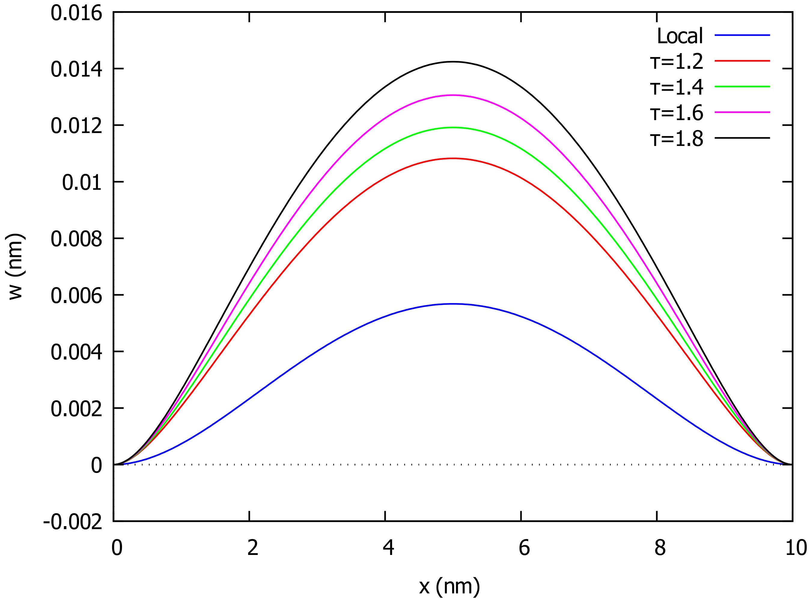
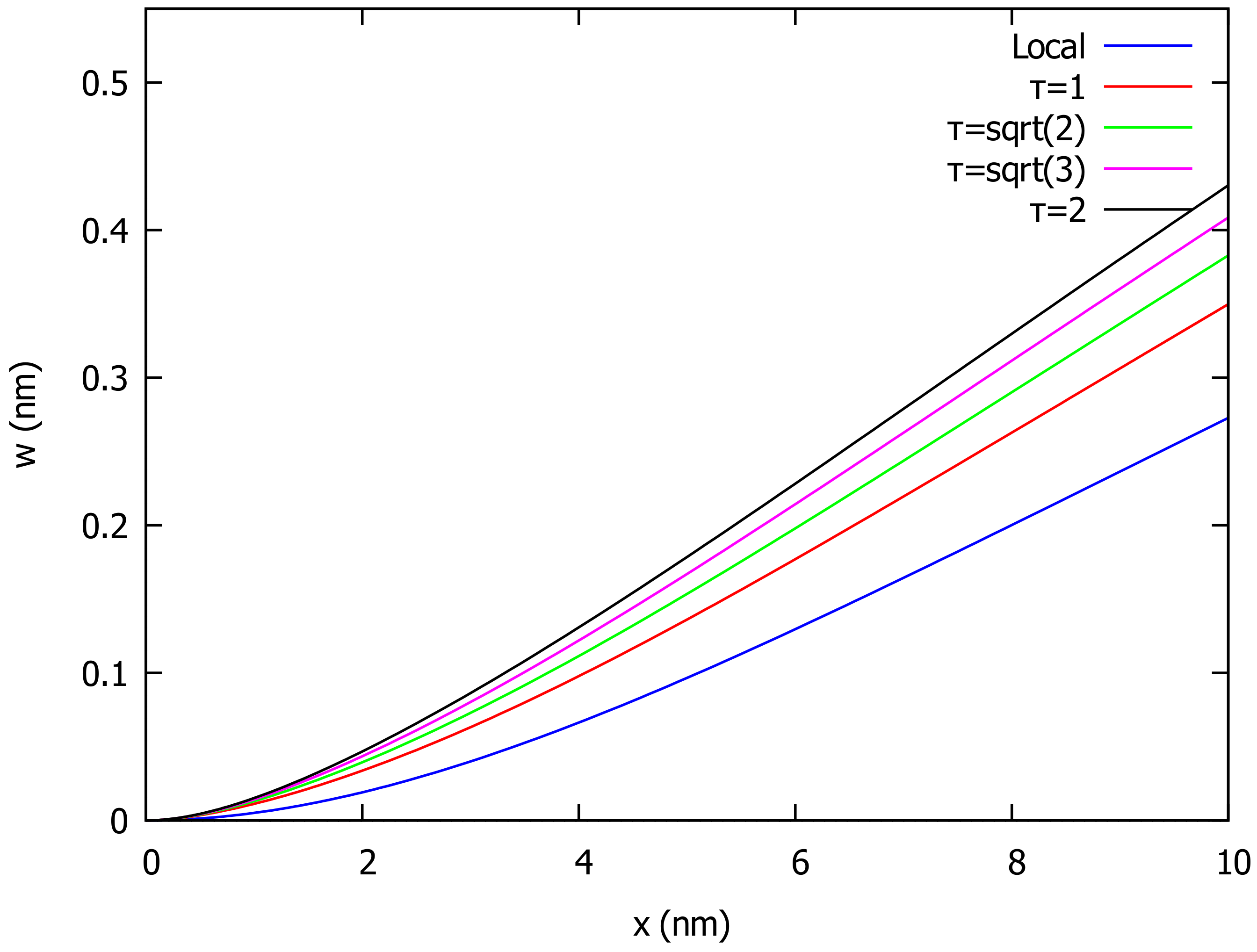
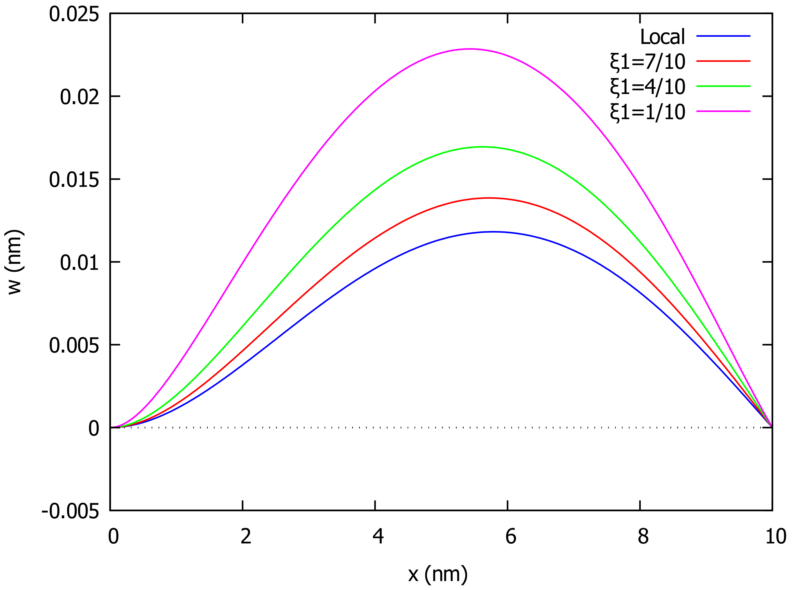
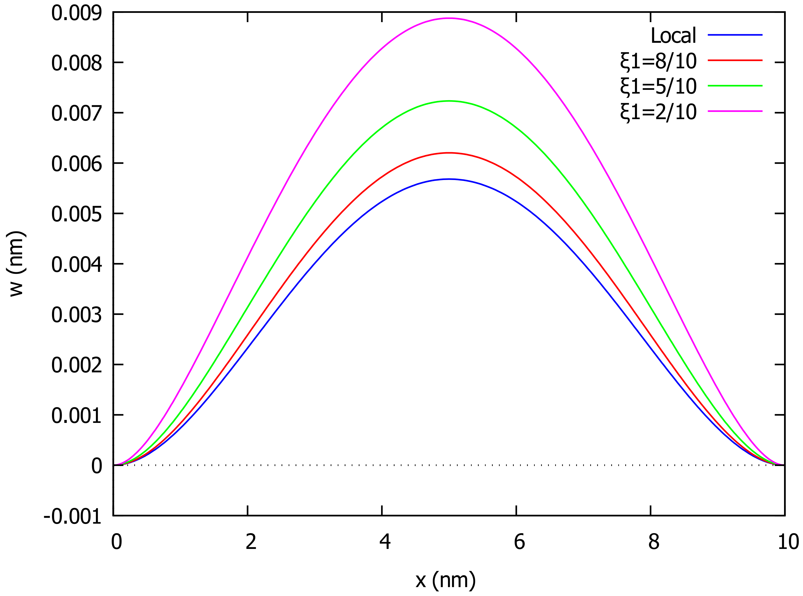
We consider three example problems corresponding to the three types of boundary conditions examined in the previous section, and for each of them, we find in closed form the transverse displacement (deflection) $w\left(x\right)$ for two different types of transverse distributed loads $q\left(x\right)$. It is noted that in all instances except the case of classical (local) theory, the solutions are generally large algebraic expressions.

Let a nanobeam have length L, height h, width b, Young’s modulus E, and a load intensity parameter $q_0$, as shown in Table 1[31]. The same table also has the intervals for the values of the nonlocal material constant $\tau$ and the parameter ${\xi }_1$ (${\xi }_1+{\xi }_2=1$). It is remarked that Wang, Q. and Liew, K.M. [28] stated that the nonlocal effect is noticeable when the length of the structure is less than 20 nm and recommended $e_{0}a<2.1$ nm, while Eringen [10] suggested a value of parameter $e_0$ to be $0.39$.

Table 1. Geometry, loading, and material parameters of the nanobeam.

L (nm)	b (nm)	h (nm)	${\mathit{q}}_0$ (nN/nm)	E (TPa)	$\mathit{\tau }={\mathit{e}}_0\mathit{a}$ (nm)	${\mathit{\xi }}_1$
10	1	1	${10}^{-4}$	5.5	$[1.0,2.0]$	$[0.1,1]$

First, we study the bending behavior of a cantilever beam (CF) for which the boundary conditions are as in (20) loaded by a transverse distributed load

$$q\left(x\right)=q_{0}orq\left(x\right)=-q_{0}sin\left(n\pi \frac{x}{L}\right),$$

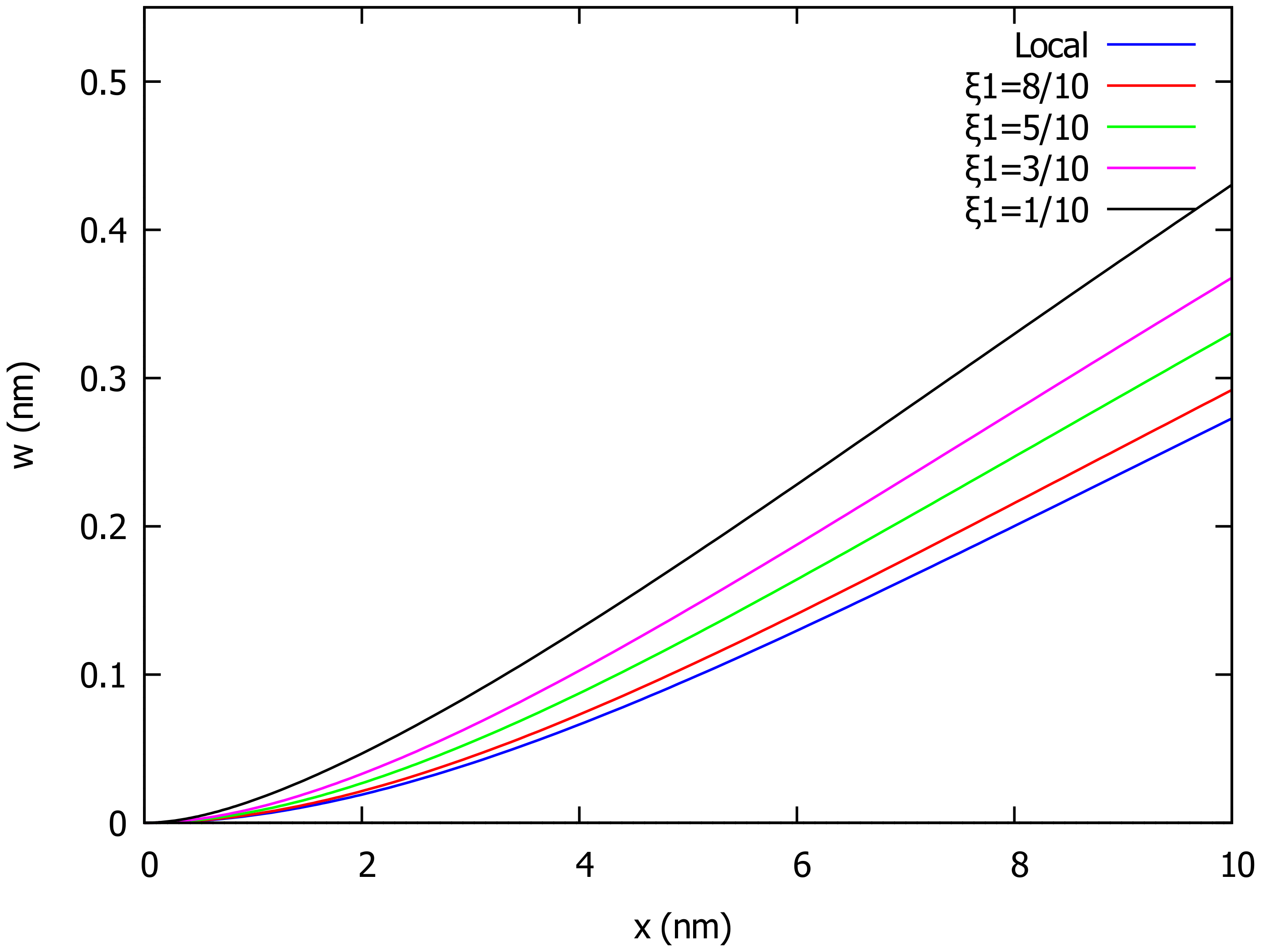
where n is a positive integer. For the case of uniformly distributed load $q\left(x\right)=q_0$, the deflection $w\left(x\right)$ throughout the beam according to local (${\xi }_1=1$) and nonlocal (${\xi }_1=0.1$) elasticity for various values of the nonlocal parameter $\tau =e_{0}a$ is depicted in Figure 1. 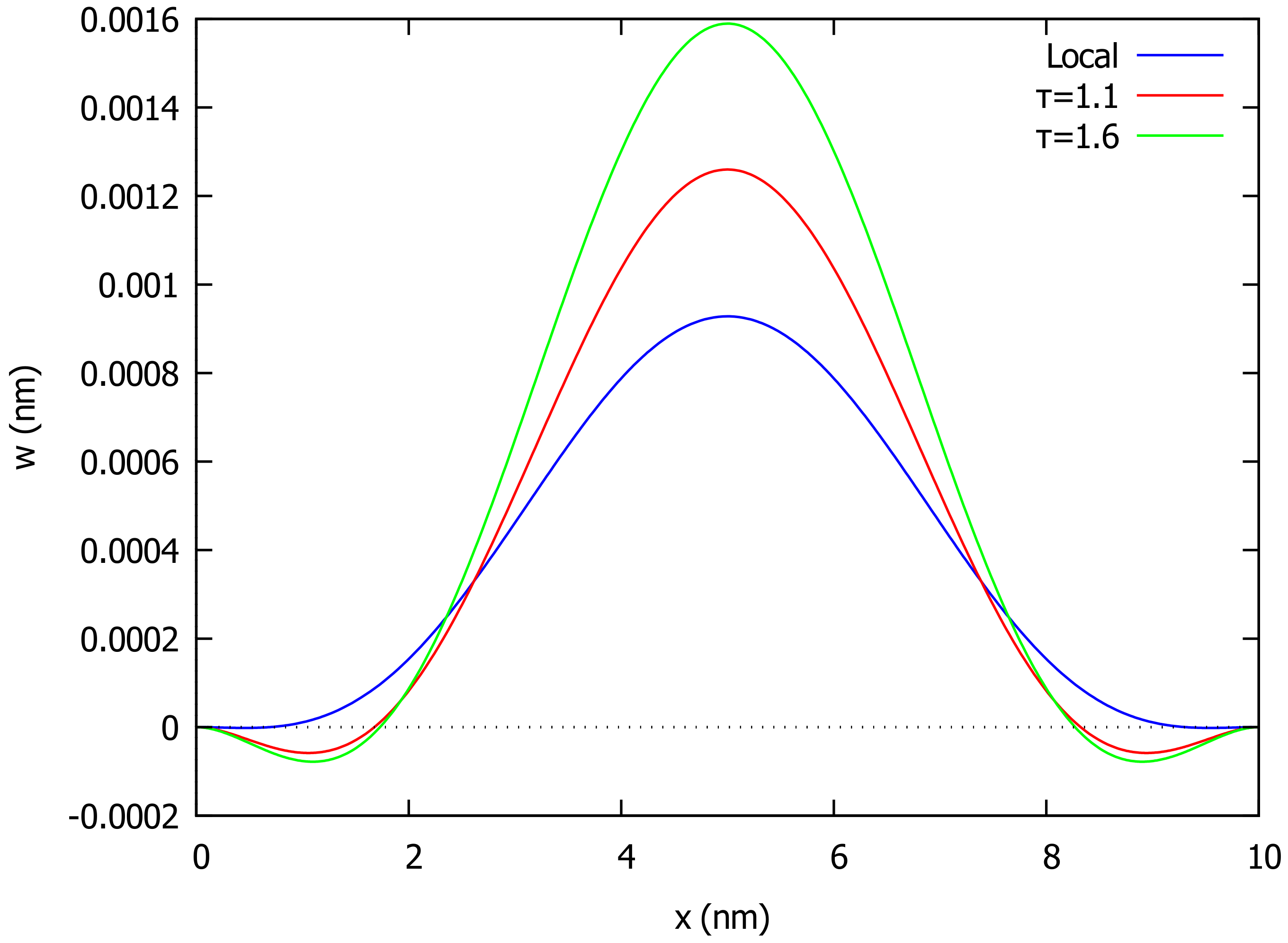Figure 2 shows the deflection $w\left(x\right)$ for $\tau =2$ and several values of the parameter ${\xi }_1$ that controls the influence of local and nonlocal integral models in the constitutive relation. In the case of a variable distributed load $q\left(x\right)$ with $n=3$, the deflection $w\left(x\right)$ is sketched in Figure 3 for different values of the nonlocal parameter $\tau$.

Figure 1. Deflection of cantilever beam (CF) under uniform load and various values of $\tau$.

Figure 2. Deflection of cantilever beam (CF) under uniform load and several values of ${\xi }_1$.

Figure 3. Deflection of cantilever beam (CF) under variable load and different values of $\tau$.

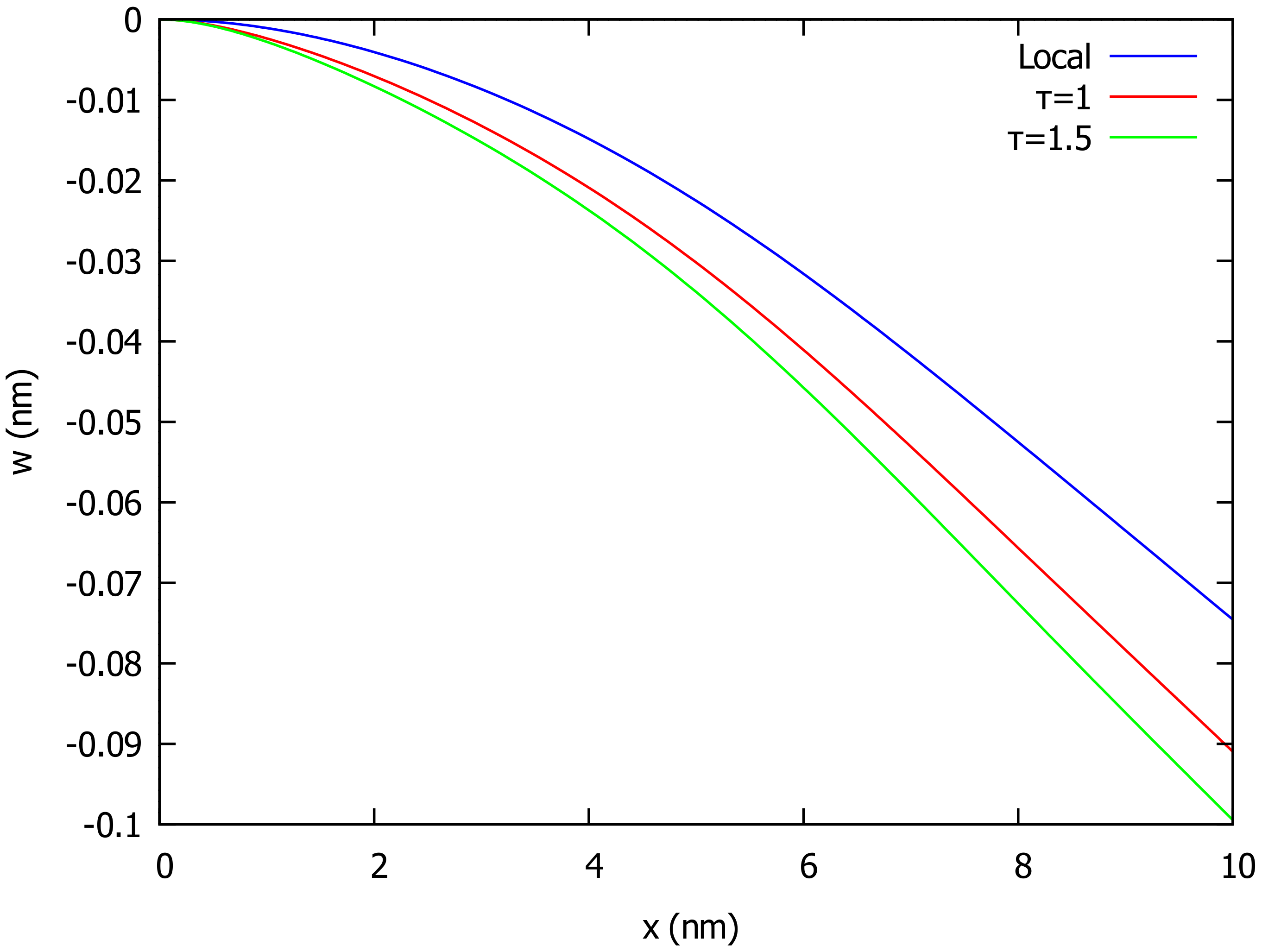
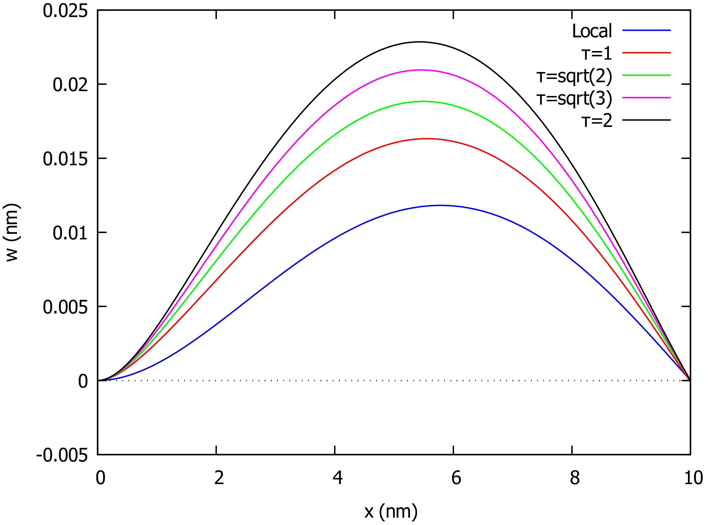
Next, we consider the case of a clamped pinned beam (CP) with the boundary conditions as in (34). For the case of uniformly distributed load $q\left(x\right)=q_0$, the deflection $w\left(x\right)$ for the whole beam in both local (${\xi }_1=1$) and nonlocal (${\xi }_1=0.1$) elasticity for several values of the nonlocal parameter $\tau =e_{0}a$ is outlined in Figure 4. In Figure 5, we give the deflection $w\left(x\right)$ for $\tau =2$ and various values of the control parameter ${\xi }_1$. 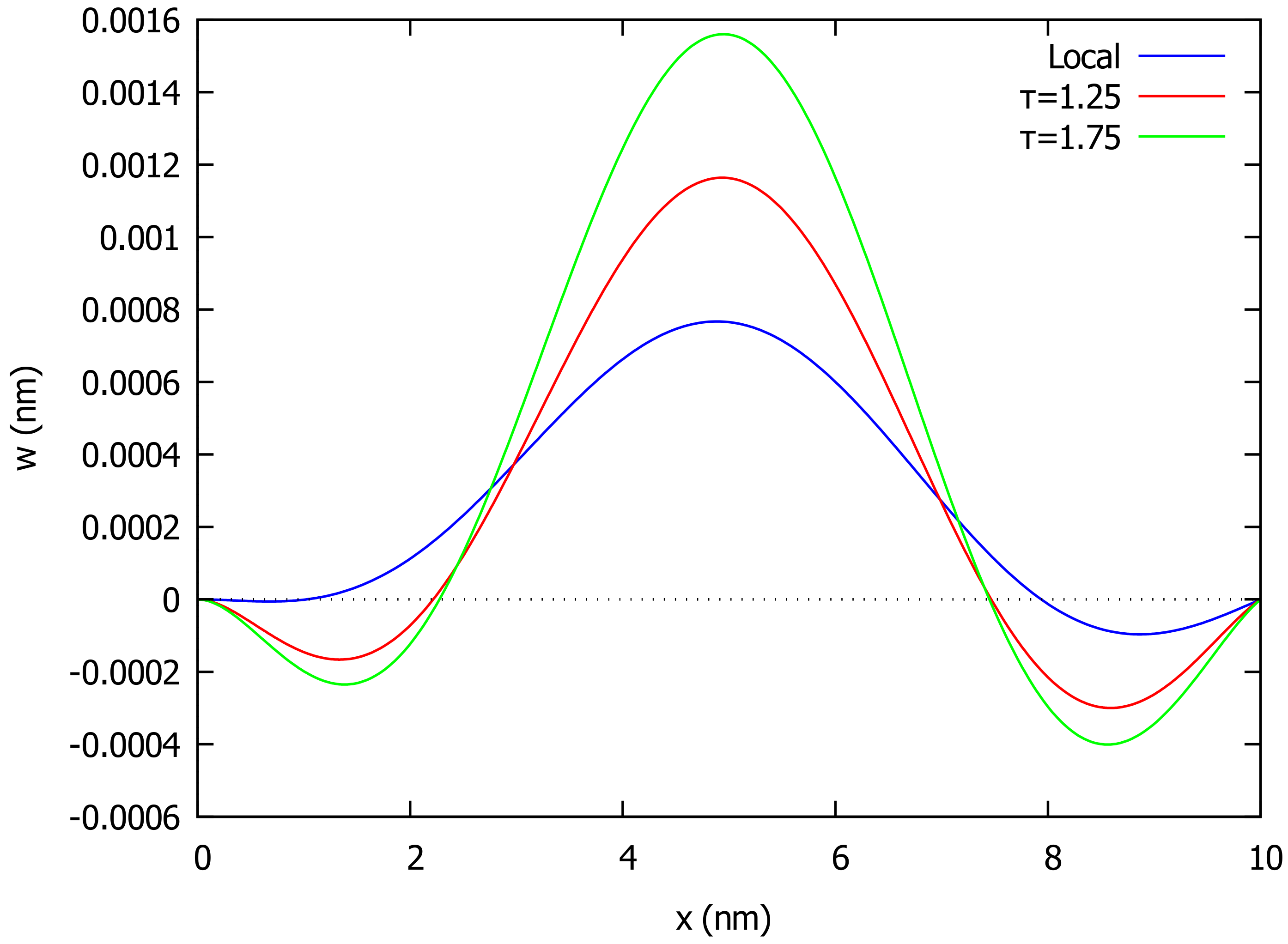The shape of deformation of the beam loaded by a variable distributed load $q\left(x\right)$ of the above type with $n=3$ is shown in Figure 6 for different values of $\tau$.

Figure 4. Deflection of clamped pinned beam (CP) under uniform load and several values of $\tau$.

Figure 5. Deflection of clamped pinned beam (CP) under uniform load and various values of ${\xi }_1$.

Figure 6. Deflection of clamped pinned beam (CP) under variable load and different values of $\tau$.

As a third example, we take the case of a clamped beam (CC) for which the boundary conditions are given in (42). In the case of a uniformly distributed load, the deflection $w\left(x\right)$ across the beam in both local (${\xi }_1=1$) and nonlocal (${\xi }_1=0.1$) theory for different values of $\tau =e_{0}a$ is given in Figure 7, while Figure 8 shows how the deflection changes as ${\xi }_1$ varies. In the case of the above variable distributed load $q\left(x\right)$ with $n=3$, the beam deforms as shown in Figure 9 in a local (${\xi }_1=1$) and nonlocal (${\xi }_1=0.2$) model for different values of the nonlocal parameter $\tau$.

Figure 7. Deflection of clamped beam (CP) under uniform load and several values of $\tau$.

Figure 8. Deflection of clamped beam (CP) under uniform load and various values of ${\xi }_1$.

Figure 9. Deflection of clamped beam (CP) under variable load and different values of $\tau$.

From the results presented, it can be concluded that in all three cases of boundary conditions and loading cases, the solutions obtained are characterized by the softening effect that the nonlocal theory has on the beam deformation. It is observed that as the nonlocal material parameter $\tau$ increases, the deformation of the beam becomes greater in all cases. In addition, as the control parameter ${\xi }_1$ approaches the unit, the influence of the nonlocal model on the beam deformation decreases, and the nonlocal solution convergences to a classical (local) solution.

Of primary interest is the case of the cantilever beam where the paradoxical behavior of the simplified nonlocal differential model has been reported by many researchers. It is noted that the cantilever beam finds many applications in nanotechnology as an actuator. It is shown here that the two-phase integral model in the case of the cantiliver beam predicts a softening effect, which is greater as the nonlocal parameter $\tau$ increases. This is consistent with the results in all other cases of boundary conditions and confirms the validity of the two-phase integral model.

5. Conclusions

The accuracy of the nonlocal differential model of Eringen’s nonlocal elasticity is questionable in some cases of loading and boundary conditions. The integral model and the two-phase integral model are valid and produce consistent results in all cases, but they have computational difficulties related to integral or integro-differential equations involved.

In this article, a technique has been presented for constructing closed-form solutions of the governing equations of the two-phase integral model of nonlocal Euler–Bernoulli nanobeams in bending, which find many applications in micro- or nano-electromechanical systems (MEMS or NEMS). The technique is based on the decomposition of the initial fourth-order integro-differential boundary value problem into two second-order boundary value problems and the use of the direct operator method for the exact solution of Volterra–Fredholm inegro-differential equations of convolution type presented in [39]. The procedure is easily programmable to any symbolic algebra system, and an algorithm has been provided.

Results have been given for three types of boundary conditions and two kinds of transverse distributed loads. It has been shown that the two-phase integral model in all cases predicts a softening effect, which is greater as the nonlocal parameter $\tau$ increases.

The technique can be used to solve easily and effectively other similar problems. Its main disadvantage is that because it is based on the Laplace transform, it is limited to classes of functions for which direct and inverse integral transformations are available.