Cost-Sensitive Variational Autoencoding Classifier for Imbalanced Data Classification

Abstract

Classification is among the core tasks in machine learning. Existing classification algorithms are typically based on the assumption of at least roughly balanced data classes. When performing tasks involving imbalanced data, such classifiers ignore the minority data in consideration of the overall accuracy. The performance of traditional classification algorithms based on the assumption of balanced data distribution is insufficient because the minority-class samples are often more important than others, such as positive samples, in disease diagnosis. In this study, we propose a cost-sensitive variational autoencoding classifier that combines data-level and algorithm-level methods to solve the problem of imbalanced data classification. Cost-sensitive factors are introduced to assign a high cost to the misclassification of minority data, which biases the classifier toward minority data. We also designed misclassification costs closely related to tasks by embedding domain knowledge. Experimental results show that the proposed method performed the classification of bulk amorphous materials well.

1. Introduction

Classification is a primary function of machine learning [1]. Some existing classification algorithms, such as support vector machines, decision trees, neural networks, and Bayesian classifiers, are widely used. However, they are typically based on the assumption that the distribution of data categories is roughly balanced [2]. However, this assumption is not valid for many practical tasks. In realistic classification tasks, the sample size of one category is likely to be much smaller than that of the other. For example, Kucat et al.’s study on detecting oil spills through satellite radar images showed that the imbalance ratio of the dataset used reached 22:1 [3]. Similarly, Perez et al. studied the identification of auto insurance fraud. The imbalanced dataset used in this study had 108,000 samples, of which, only 7.4% were fraudulent samples. There is also a large amount of imbalanced data in text classification, medical diagnosis, network intrusion monitoring, and other fields [4].

Traditional classification algorithms consider overall classification accuracy as the learning goal. When the classification data are imbalanced, traditional machine learning algorithms pay more attention to the majority-class samples and ignore the minority-class samples to increase the overall classification accuracy [5]. Thus, traditional machine learning algorithms do not perform well in the task of identifying members of minority data classes. In addition to classification accuracy, in many cases, the cost of the misclassification of a minority sample is much greater than that of the misclassification of a majority sample. For example, in medical diagnosis tasks, the identification of minority-class (ill) samples as majority-class (normal) samples may seriously delay the treatment time of patients and cause major medical accidents. Therefore, if the misclassification cost of minority samples is treated equally to the misclassification cost of majority samples, significant errors in the practical application of the classifier may result. The imbalanced data classification problem focuses on the performance of classifiers in the case of imbalanced data categories, and research on this problem has attracted considerable interest as a popular topic in the field of machine learning [6].

Research on imbalanced data classification has been mainly carried out on the levels of data, algorithms, and evaluation criteria. Existing algorithms for imbalanced data mainly involve improvements at a single level. In this paper, an imbalanced data classification algorithm termed a cost-sensitive variational autoencoding classifier (cost-sensitive VAE) is proposed, which involves both the data level and algorithm level. The main contributions of the present work are summarized as follows.

-

We propose a cost-sensitive variational autoencoding classifier for imbalanced data classification. In contrast to traditional imbalanced classification algorithms, which usually involve only one level, the proposed approach adapts to imbalanced data at the levels of data and algorithms. A cost-sensitive matrix is introduced to improve the recognition rate of minority samples, and data can be generated by generators to expand the minority classes from the data level. Experiments 1 and 2 show that this method has a good classification performance on imbalanced datasets. Experiment 1 confirmed that each category in the classification task exhibited good Precision, Recall, and F1-score by this method, with the F1-score, Precision, and Recall of the minority class (BMG) being 0.9432, 0.9644, and 0.9239, respectively. Experiment 2 confirmed that the cost-sensitive factor $\alpha$ in this method has a beneficial effect on the Precision, Recall, and F1-score of each category, which affects minority categories more obviously than majority categories.

-

A cost-sensitive matrix design based on domain-knowledge embedding is proposed. In traditional methods, the determination of the misclassification cost is closely related to the number of samples in each class. Usually, the number of samples in the dataset or the proportion of samples of each class is taken as the misclassification cost, which cannot reflect the real class distribution characteristics of data well and cannot guarantee the effect of cost-sensitive learning. The proposed approach includes misclassification costs closely related to tasks by embedding domain knowledge. The design and performance of the cost matrix is improved by embedding domain knowledge. Experiment 3 verifies that the cost matrix embedded with domain knowledge can improve the performance of the proposed classifier.

In this paper, we analyze the classification of imbalanced data and propose a classification algorithm for imbalanced data based on a cost-sensitive variational autoencoder. The remainder of this paper is organized as follows. In Section 2, we discuss the related work on imbalanced data classification and examine some classic algorithms. In Section 3, the proposed cost-sensitive variational autoencoding classifier is introduced, and the theoretical basis of the algorithm is described. In Section 4, the performance of the cost-sensitive variational autoencoding classifier algorithm is tested experimentally. In Section 5, we summarize the conclusions and suggest possible avenues for future research.

2. Related Work

Thus far, the related research on imbalanced data classification has mainly considered three different levels, including data, algorithm, and discriminant criterion levels.

2.1. Research on Imbalanced Data Classification at the Data Level

At the data level, classification is mainly used to change the distribution of training data by sampling the original data to eliminate or reduce data imbalance, including over-sampling and under-sampling methods.

The over-sampling method improves the classification performance of minority classes by increasing the number of minority samples. The simplest method is to copy minority samples directly. The disadvantage of this method is that it simply copies minority samples without adding any new information to minority classes, which may lead to overfitting. The improved over-sampling method solves the above problems to some extent by adding random Gaussian noise to minority classes to generate new synthetic samples. For example, the SMOTE algorithm proposed by Chawla et al. is a classic over-sampling method [7]. SMOTE generates a new minority sample without repetition by randomly selecting samples of the same kind of close neighbours for interpolation, which can overcome the overfitting problem of the random over-sampling method to some extent. However, the SMOTE method also has several problems, such as over-generalization, sample overlap, and noise. To solve the above problems, several improved methods have been developed based on SMOTE, such as Borderline-SMOTE [8] and SMOM [9]. In [10], the classification performance of minority classes is addressed by selecting suitable neighbours in the minority classes with which to increase the number of minority classes and generate new synthetic samples using the firefly algorithm. Reference [11] proposed a method that combines over-sampling technology and instance selection techniques to classify imbalanced data streams. The method selects data streams from different classes to form data chunks using the over-sampling technique, and then selects the data chunks for classifier learning using the instance selection techniques. Reference [12] proposed a density-based mixed sampling method that deletes high-density samples from the majority classes and samples low-density samples from the minority classes. This eliminates the noise in the two classes and maintains the structural balance of the classes to the maximum extent, improving the performance of the classifier.

In contrast, the under-sampling method improves the classification performance of the minority classes by reducing the number of majority-class samples. The simplest method is to remove some majority-class samples randomly to reduce the size of the majority class, which has the disadvantage of some important information of the majority class being lost and existing information not being able to be fully utilized [13]. Therefore, many improved under-sampling methods have been proposed. Kumat and Matwin proposed a one-sided sampling method to remove noise, boundary, and redundant samples in the majority-class samples. The basic idea of the algorithm is to divide the majority samples into noise, boundary, and safety samples, and to delete the boundary and noise samples from the majority samples without deleting useful samples as much as possible in order to achieve a better classification performance than random under-sampling [14]. In [15], an under-sampling algorithm based on clustering was proposed. First, the training set is divided into several clusters using a clustering method, and each cluster contains a certain number of majority and minority classes. For each cluster, all of the minority classes are removed, and the majority classes in the cluster are undersampled according to certain rules. Finally, the samples taken from each cluster are combined to obtain a new training set.

2.2. Research on Imbalanced Data Classification at the Algorithm Level

From the perspective of algorithms, the strategies adopted mainly include cost-sensitive and ensemble learning methods.

2.2.1. Cost-Sensitive Method

When dealing with the problem of imbalanced data classification, the traditional classifier algorithms treat the misclassification costs of different categories equally and aim to reduce the global classification error rate. Therefore, owing to the small number of samples of minority classes, the traditional classification algorithms have a low recognition rate of minority classes. However, in practical tasks, different classification errors result in different degrees of loss, and the cost of minority categories being misclassified is far greater than the cost of the majority categories being misclassified in general. For example, in medical diagnosis, the cost of misclassifying sick samples (minority samples) as healthy samples (majority samples) is much greater than that of misclassifying healthy samples (majority samples) as sick samples (minority samples). The basic idea of cost-sensitive learning is to assign a high misclassification cost to the minority classes and a low misclassification cost to the majority classes, and then to minimize the total misclassification cost as the training and optimization goal of the algorithm, so as to improve the classification performance of minority classes. At present, the research on cost-sensitive learning has mainly focused on two aspects: directed cost-sensitive learning and meta cost-sensitive learning.

The main method of directed cost-sensitive learning is to change the internal structure of the traditional classifier model by introducing a cost-sensitive factor based on the traditional classification algorithm and transforming the traditional training goal of reducing the global classification error rate into the training goal of reducing the global classification error cost. Researchers have proposed cost-sensitive versions of various learning models, such as a support vector machine (SVM), decision tree, and neural network [16,17]. For example, in [18], a new cost-sensitive decision tree approach that minimized the sum of misclassification costs while selecting the splitting attribute at each non-terminal node was developed. The performance of the proposed method was compared with that of the traditional classification model on a real credit card dataset, and better experimental results were obtained. Reference [19] assigned different costs to false positive errors and false negative errors as specified by a ratio to estimate a classifier that minimized the weighted error. In [20], the concept of a weighted SVM (W-SVM) was proposed to move the classification boundary to the majority classes to solve the defect of the SVM algorithm not being able to treat each class differently according to the importance of each class, and to improve the prediction accuracy of models for the data of minority classes. In [21], a cost-sensitive back-propagation neural network (CSBPNN) algorithm for multi-category imbalanced data classification was proposed. This algorithm introduced a misclassification cost such that the output threshold moved toward the higher cost classes to ensure that they were classified correctly. References [22,23] proposed a novel cost-sensitive algorithm that introduced cost information not only in the prediction stage, but also in the deep learning model stage.

Directed cost-sensitive learning makes the traditional classification algorithm suitable for imbalanced data by modifying the internal structure of the classifier. However, as some algorithms are difficult to modify directly, the concept of meta cost-sensitive learning has been proposed. On the premise of not changing the existing learning algorithm, meta cost-sensitive learning converts the misclassification cost of the class into the sample weight. It weights each sample according to the misclassification cost of the class to which it belongs, and then reconstructs the original dataset according to the weight. The disadvantage is that the process of reconstruction changes the distribution of samples and sometimes loses some useful sample information. MetaCost [24] is a typical meta cost-sensitive learning method. The idea of MetaCost is derived from the Bayesian risk theory. The main steps are as follows [25]. First, the original training set is randomly sampled M times to obtain M sub-datasets, a base classifier is trained for each sub-dataset to obtain M base classifiers, and then all base classifiers predict the original data and average all predicted probability values (if parameter q is set to true, all models directly predict all data; otherwise, it is set to false and only its own training data are predicted). Then, the prediction probability of the sample is multiplied by the cost-sensitive matrix and the category with the least loss is taken as the new label of the sample to reconstruct the sample. By estimating the posterior probability density of training samples, the ideal category of each training sample is calculated by combining the cost matrix; then, the original training sample category is modified according to the ideal category to obtain the new training set. Finally, the new training set is learned by using the classifier based on the error rate.

2.2.2. Ensemble Learning Method

The main idea of the ensemble learning method is to train multiple base learners and then to coordinate the results of multiple base learners to obtain the final result. Ensemble learning is used for imbalanced data classification, mainly because of its concept of integration. It combines the preferences of multiple classifiers and combines classifiers with existing imbalanced data classification methods to deal with the task of imbalanced data classification [26].

Ensemble learning methods can be divided into heteromorphic and homomorphic types, according to the category relationship between basic classifiers [27]. Heteromorphic ensemble learning refers to the use of a variety of different classifiers for integration, whereas homomorphic ensemble learning refers to the integration of the basic classifier with the same kind of classifier with different parameters. Different integration methods have their own advantages in the classification of imbalanced data.

In heteromorphic integration methods, each basic classifier has its own unique characteristics; therefore, for a particular type of data set, one of the basic classifiers will be more efficient than the others. The heteromorphic ensemble learning method is always combined with a cost-sensitive method to change the weight of each base classifier in the next iteration according to the performance of each base classifier in each iteration until the final result is integrated at the end of the iteration. The classical algorithm is AdaBoost [17,28,29]. AdaBoost has multiple iterations, with each iteration learning a classifier and updating the weight of the sample based on the performance of the current classifier. The update strategy is as follows. In each iteration classification, the weight of the correctly classified samples is reduced, and the weight of the incorrectly classified samples is increased. The final model is a weighted linear combination of multiple iteration models. AdaCost [30] modifies the weight-update strategy of the AdaBoost algorithm. In AdaBoost, the weight of the correctly classified sample is reduced to the same proportion, and the weight of all misclassified instances is also increased by the same proportion. By contrast, the adjustment strategy of AdaCost is to greatly increase the weight of the misclassified samples at a high cost. Researchers have also proposed many improved versions of AdaCost, such as AdaC1, AdaC2, and AdaC3 [31].

In the homomorphic ensemble learning method, the strategy for imbalanced data is to combine sampling and integration, to generate multiple subsets through a series of sampling of the original training set, then to train the base classifier with different subsets, and finally to output the final result through voting or merging. Typical algorithms include SMOTEBoost [32]. The method is based on an imbalanced data processing method, and the sampling technology is embedded in the boosting algorithm, which changes the data distribution used to train the next classifier in the direction of small classes. Some studies have shown that the integration interval is the key factor influencing the integrated learning classification performance [33]. Chen et al. [34] combined SMOTE with bagging, boosting, and other methods, and proposed a method designed to change the sample weight by changing the data sampling interval, which can improve the classification accuracy of a few types of samples.

2.3. Research on Imbalanced Data Classification at Discriminant Criterion Level

The method of evaluation is to judge the performance of the algorithm using a special discriminant criterion. Accuracy is a commonly used evaluation standard for classification problems. It reflects the overall classification performance of the classifier on the dataset, but it cannot accurately reflect the classification performance of an imbalanced dataset. Therefore, more reasonable evaluation criteria should be proposed for imbalanced data. Commonly used criteria include Recall, Precision, F1-score, G-mean, and area under the curve(AUC).

3. Method and Algorithm

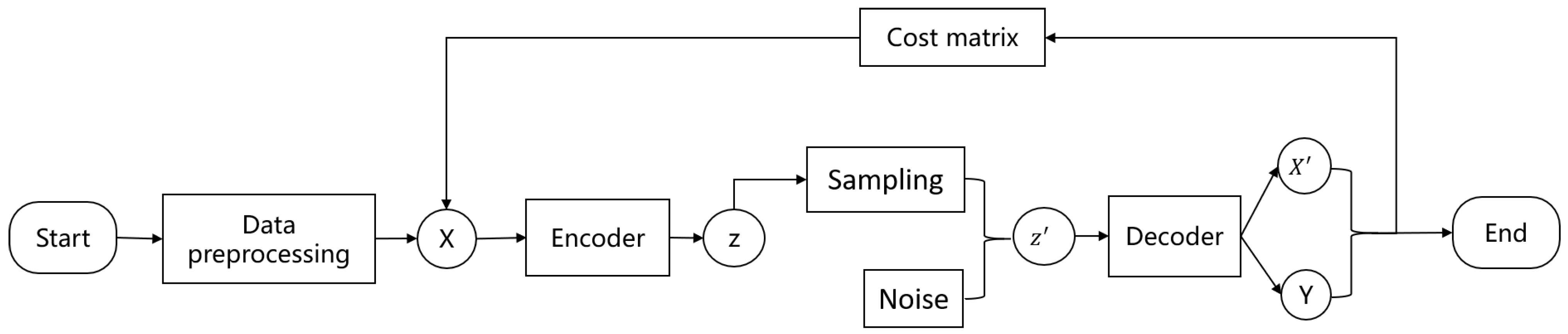
3.1. Overall Model

The cost-sensitive variational autoencoding classifier (cost-sensitive VAE) proposed in this paper is divided into three parts: encoder, decoder, and cost-sensitive modules. The function of the encoder is to obtain the distribution of the hidden variable Z of the original data X. The decoder’s function is to sample the hidden variable Z and then reconstruct the data X and obtain the label Y of the data. The function of the cost-sensitive module is to adapt to the situation of imbalanced data. A flow chart of the proposed cost-sensitive VAE classifier is shown in Figure 1.

The cost-sensitive method adopts a cost matrix; the form of the matrix is shown in Equation (1). The order c of the matrix is the same as the number of data categories. The element $cost[i,j]$ ($1\le i,j\le c$) in the matrix represents the cost of a sample originally classified as class i being misclassified as class j.

$$Cost=\left[\begin{array}{ccccc}cost[1,1]& \cdots & cost[1,j]& \cdots & cost[1,c]\\ ⋮& & ⋮& & ⋮\\ cost[i,1]& \cdots & cost[i,j]& \cdots & cost[i,c]\\ ⋮& & ⋮& & ⋮\\ cost[c,1]& \cdots & cost[c,j]& \cdots & cost[c,c].\end{array}\right]$$

(1)

The cost function of this model is shown in Equation (2).

$$L=-E_{z\sim q\left(z\right|x)}\left[logP\left(x\right|z)\right]+KL\left(q\left(z\right|x)\right|\left|p\left(z\right)\right)+\psi \ast L(\widehat{y},y)\ast cost[y,\widehat{y}].$$

(2)

where $-E_{z\sim q\left(z\right|x)}\left[logP\left(x\right|z)\right]$ represents the minimized reconstruction error of the original data. KL is the Kullback–Leibler divergence, which is used to measure the difference between two probability distributions in the same event space; thus, $KL\left(q\right(z\left|x\right)\left|\right|p\left(z\right))$ represents whether the distribution of the hidden variable Z is close to the Gaussian distribution. $L(\widehat{y},y)$ represents the model classification loss function (in this paper, the cross-entropy loss function was adopted), $cost[y,\widehat{y}]$ represents the classification cost, and $\psi$ represents the importance of the classification task.

3.2. Cost-Sensitive Variational Auto-Encoder Classifier

This section presents, in detail, the construction of the cost-sensitive variational autoencoding classifier.

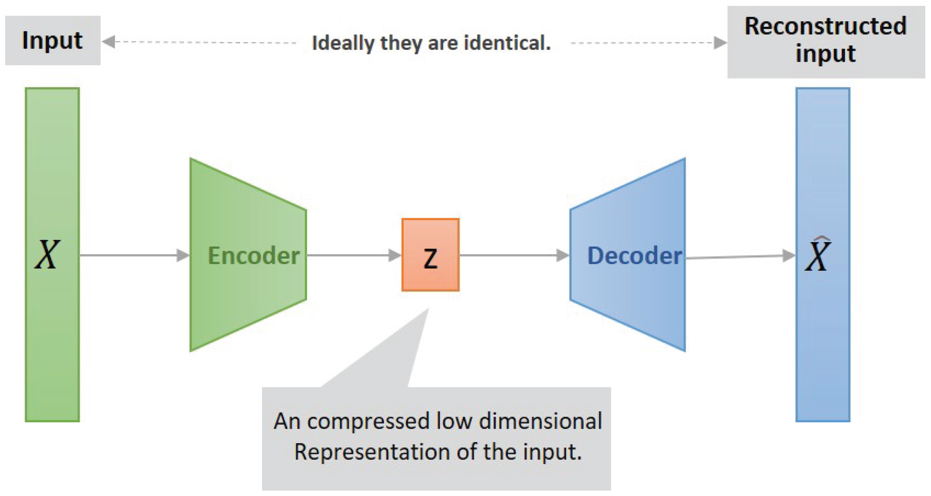
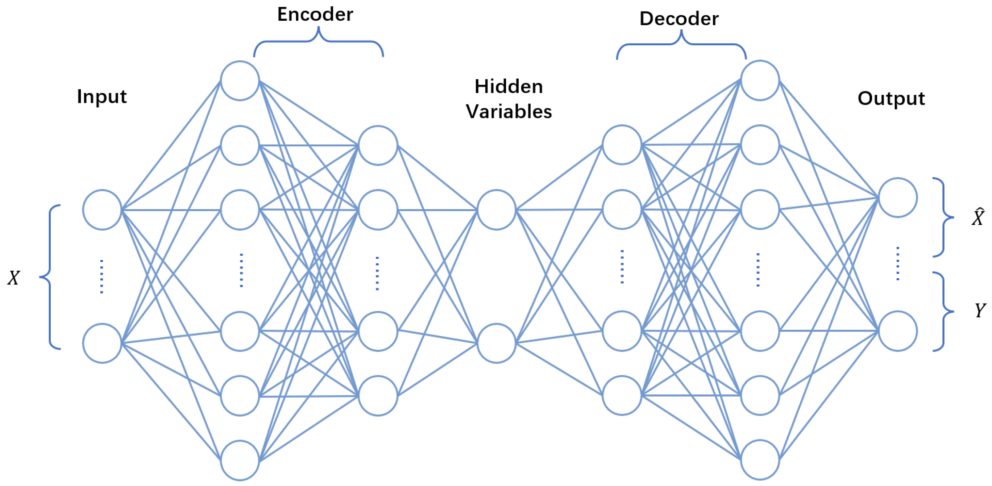
3.2.1. Variational Autoencoder

Variational autoencoder (VAE) is an important generation model proposed by Diederik P. Kingma and Max Welling in 2013 [35]. The graph model of VAE is shown in Figure 2, where x denotes the data that we can observe, z denotes the hidden variable, and VAE assumes x is produced by the hidden variable z. $z\to x$ is the generation model, which is the working process of the decoder from the view point of the autoencoder, and $x\to z$ is the recognition model, which is the working process of the encoder from the view point of the autoencoder. $\theta$ and $\omega$ represent the parameters of the process and N stands for N samples.

The basic idea of the VAE is to assume that the data sample X is generated by the hidden variable Z in a certain way, i.e., $X=g\left(Z\right)$. If we can learn the distribution of the hidden variable Z from the original data, i.e., determine the f in $Z=f\left(X\right)$, then we can obtain a new $\widehat{Z}$ by sampling on Z and generate new data by $\widehat{X}=g\left(\widehat{Z}\right)$. The VAE model is shown in Figure 3 as being mainly composed of encoder and decoder. The encoder accepts the input data X and outputs the distribution of the hidden variable. In the VAE, it is assumed that the hidden variable z satisfies the Gaussian distribution, so the encoder outputs the expectation and variance of the Gaussian distribution. The decoder accepts the mean of the hidden variable Z, and then outputs the reconstructed sample of the input data ($\widehat{X}$), where X and $\widehat{X}$ should be as close as possible. In the process of data generation, a new $\widehat{Z}$ is first sampled from the distribution obtained by the encoder and then input into the decoder to generate new sample data.

We assumed that there were some hidden variables z, but we did not know what the distribution was, and all we could observe was sample x. Therefore, we had to derive the distribution of z given x; specifically, we had to calculate $p\left(z\right|x)$. $p\left(z\right|x)$ can be given by Equation (3).

$$p\left(z\right|x)=p(x\left|z\right)\ast p\left(z\right)/p\left(x\right).$$

(3)

However, this integral of the Equation (3) cannot be calculated directly because we cannot directly calculate $p\left(x\right|z)$ (x may have a high dimension). We could use the MCMC method to sample and then estimate the integral directly; however, in practice, this method is not feasible because it would be too slow. To solve this problem, we introduced the variational method by introducing an additional encoder $q\left(z\right|x)$ to model the relationship between x and z; that is, we used $q\left(z\right|x)$ to approximate $p\left(x\right|z)$. Therefore, our goal is as shown in Equation (4).

$$minKL\left(q\right(z\left|x\right)\left|\right|p\left(z\right|x\left)\right).$$

(4)

KL is the Kullback–Leibler divergence, which is used to measure the difference between two probability distributions in the same event space. The KL divergence is an asymmetric measure of the difference between two probability distributions. For $q\left(z\right|x)$ to be as close as possible to $p\left(x\right|z)$, the KL value must be minimized. According to the calculation formula of KL divergence, Equation (5) can be obtained.

$$\begin{array}{cc}\hfill KL\left(q\right(z\left|x\right)\left|\right|p\left(z\right|x\left)\right)& =\int q(z|x)\ast logq(z|x)dz+logp(x)\ast \int q(z|x)dz\hfill \\ \hfill & -\int q(z|x)\ast log(p(z|x)\ast p(z))dz\hfill \end{array}$$

(5)

Due to the fact that $\int q(z|x)dz$ is equal to one, and the value of $logp(x)$ is fixed, the goal can be converted to minimizing the first and third terms of Equation (5). Setting the target as L, Equation (6) can be obtained.

$$L=\int q(z|x)\ast logq(z|x)dz-\int q(z|x)\ast log(p(z|x)\ast p(z))dz$$

(6)

Then, by dividing the first and second terms by $p\left(z\right)$, Equation (6) is transformed to obtain Equation (7), as shown below.

$$\begin{array}{cc}\hfill L& =\int q(z|x)\ast log(q(z|x)/p(z))dz-\int q(z|x)\ast logp(z|x)dz\hfill \\ \hfill & =-E_{Z\sim q\left(z\right|x)}\left[logP\left(x\right|z)\right]+KL\left(\right(q\left(z\right|x)\left|\right|p\left(z\right)\left)\right)\hfill \end{array}$$

(7)

The $KL\left(q\right(z\left|x\right)\left|\right|p\left(z\right))$ signifies that the hidden variables z are close to a Gaussian distribution, and the $-E_{Z\sim q\left(z\right|x)}\left[logP\left(x\right|z)\right]$ represents the minimized reconstruction error of the original data.

3.2.2. Variational Auto-Encoder Classifier

VAE can be seen as a neural network in nature, so it can be used as a classifier in addition to generating new samples as a generation model. A new output layer is added after the VAE model for data classification, and then a classification loss item (such as the cross entropy loss function) is added on the basis of the original loss function to convert the VAE model into a classifier. The model of the classifier is shown in Figure 4, where X represents the input data, Y represents the label of the input data, and $\widehat{X}$ represents the reconstruction of the input data. Due to the fact that a new classification task is added to the original VAE model, the cost function of the original model needs to be changed. The changed cost function is shown in Equation (8), where $L(\widehat{y},y)$ represents the loss function of the model classification, and the cross-entropy loss function was used in this study. $\psi$ indicates the importance of the classification task.

$$L=-E_{Z\sim q\left(z\right|x)}\left[logP\left(x\right|z)\right]+KL\left(q\left(z\right|x)\right|\left|p\left(z\right)\right)+\psi \ast L(\widehat{y},y)$$

(8)

3.2.3. Classifier Design Based on Cost-Sensitive Factor

Considering the data imbalance, cost-sensitive factors can be introduced on the basis of the above model to adapt to the imbalanced data and improve the classification performance of the model on the imbalanced data. Commonly used cost-sensitive factors include cost sampling, cost matrix, learning rate adjustment, and threshold shift. A cost-sensitive method based on a cost matrix was adopted in this study. The cost matrix presents the cost of category misclassification in the form of a matrix. The form of the cost matrix is given in Equation (1). The number c represents the number of data categories, e.g., in a binary classification task, and the cost-sensitive matrix is a $2\ast 2$ matrix. The element $cost[i,j]$ in the matrix represents the cost of category i samples being misclassified into category j. To improve the classification performance of the minority class, the overall design idea of the cost-sensitive matrix is to add a high cost to the minority class and a low cost to the majority class. In the cost-sensitive variational autoencoder proposed in this paper, domain knowledge was introduced to design the cost-sensitive matrix. The specific operation method is described in detail in the experimental section (Section 4.2). After the cost sensitivity is added, the cost function of the model is as shown in Equation (9).

$$L=-E_{Z\sim q\left(z\right|x)}\left[logP\left(x\right|z)\right]+KL\left(q\left(z\right|x)\right|\left|p\left(z\right)\right)+\psi \ast L(\widehat{y},y)\ast cost[y\underline{}true,y\underline{}predict]$$

(9)

where $-E_{Zq\left(z\right|x)}\left[logP\left(x\right|z)\right]$ is the reconstruction error of the input data, $KL\left(q\right(z\left|x\right)\left|\right|p\left(z\right))$ is the KL error, $L(\widehat{y},y)$ is the classification error, $\psi$ is the weight of the classification error, and $cost[y\underline{}true,y\underline{}predict]$ is the corresponding misclassification cost.

In summary, we obtained the overall algorithm for the cost-sensitive VAE. First, the cost-sensitive matrix was designed based on the domain knowledge. Next, the original data x were input, and the distribution of the hidden variable z was obtained by the encoder. Then, the new hidden variable $z^{\prime }$ was obtained by sampling on the distribution of the hidden variable. Finally, the reconstruction $\widehat{x}$ and the label $\widehat{y}$ of the original data x were obtained through the decoder. The specific procedure utilized by the cost-sensitive VAE is shown in Algorithm 1.

Algorithm 1 Cost-sensitive Variational Autoencoding Classifier
Input: training set $X={\left\{x_t\right\}}_{t=1}^N$, corresponding labels $Y={\left\{y_t\right\}}_{t=1}^N$, loss weight $\psi$, cost matrix $cost$
Output: Model ${\theta }_{final}$, ${\omega }_{final}$
1:	Initialize model parameters $\theta$ and $\omega$
2:	fort in $iteration$ do
3:	Sample $x_t$ in the minibatch: ${\mathit{out}}_i=fp(x_i,{\theta }_i)$.
4:	Encoder: $u_{z_t},{\sigma }_{z_t}\leftarrow f_{\omega }\left(x_t\right)$.
5:	Sampling: $z_t\leftarrow u_{z_t}+ϵ\odot {\sigma }_{z_t},ϵN\left(0,I\right)$.
6:	Decoder: ${\widehat{x}}_t,{\widehat{y}}_t\leftarrow f_{\theta }\left(z_t\right)$.
7:	Compute reconstruction loss:
8:	${\mathcal{L}}_{rec}=-log{p}_{\theta }\left(\left.x_t\right|z_t\right)$.
9:	Compute KL loss:
10:	${\mathcal{L}}_{KL}=KL(q\left(z_t\right|x_t)\left|\right|p\left(z_t\right))$.
11:	Compute classification loss:
12:	${\mathcal{L}}_{cla}=L(\widehat{y_t},y_t)$.
13:	Fuse the three losses:
14:	$\mathcal{L}(\theta ,\omega )=-log{p}_{\theta }\left(\left.x_t\right|z_t\right)+KL(q\left(z_t\right|x_t)\left|\right|p\left(z_t\right))+\psi \ast L(\widehat{y_t},y_t)\ast cost[y\underline{}true,y\underline{}predict]$.
15:	Back propagation: $gra{d}_t=bp({\theta }_t,{\omega }_t)$.
16:	Update: ${\theta }_{t+1}={\theta }_t-lr\ast gra{d}_t$.
17:	end for
18:	return Model with parameters ${\theta }_{final}$ and ${\omega }_{final}$

4. Experimental Setup and Analysis of Results

In this section, we detail the experiments conducted to verify the performance of the proposed cost-sensitive VAE classifier on an imbalanced dataset. The cost-sensitive VAE classifier was compared with some existing classification algorithms, such as SVM, k-nearest neighbour, decision tree, Bayesian classifier, and random forest. This section presents the dataset used, experimental methods, experimental environment, and results obtained.

4.1. Experimental Datasets

The data used in the experiment were bulk amorphous materials data. There were 5935 pieces of data in the dataset, each of which included 94 atomic features and a phase formation label including bulk metallic glass (BMG), crystalline alloy (CRA), and ribbon metallic glass (RMG). The purpose of the experiment was to identify the phase formation of a certain material. This dataset contained 5935 pieces of data, including 675 pieces of BMG, 1552 pieces of CRA, and 3708 pieces of RMG. Thus, it was an imbalanced dataset with a class-imbalanced ratio of 1:2.29:5.49. The dataset was prepared through the following pre-processing steps. The label attribute was changed to the corresponding one-hot encoding, and each feature of the data was normalized to the interval [−1, 1].

4.2. Design of Cost Sensitive Factor

This experiment involved three categories of classification. Its purpose was to classify the material dataset; that is, to identify the phase formation of the samples, including BMG, RMG, and CRA. Therefore, the cost matrix was a $3\ast 3$ matrix, which is listed in

Table 1. Cost matrix for amorphous alloy phase classification.

	BMG	CRA	RMG
BMG	1	High	High
CRA	Medium	1	Medium
RMG	Low	Low	1

. The diagonal element in the table was set to one instead of zero to prevent the cost of the classification task from being excessively small (i.e., preventing the value of $L(\widehat{y},y)$ from being excessively small), resulting in a serious imbalance in the importance ratio of the three tasks of calculating the distribution of hidden variables, reconstruction of input data, and classification of the data. When the main diagonal element of the cost matrix is set to zero, if the number of correctly classified samples is too large, the value of $L(\widehat{y},y)$ will be too small. Thus, the proportion of the classification task in the total task was accordingly reduced, and the classification task was ignored, which, in turn, led to the number of correctly classified samples and the classification performance being reduced.

As shown in the previous section, the cost-sensitive VAE classifier assigns different cost-sensitive factors to the three types of samples, as shown in Table 1, where High > Medium > Low. In this paper, the determination of the value of the three parameters High, Medium, and Low is mainly based on the method of domain knowledge embedding, and the relationship between the size of each misclassification cost is confirmed by analyzing the possible consequences of mutual misclassification between the categories. Relationships are then established between the three, and the values of the three are obtained through a grid search method.

Among the three categories of experimental data, BMG is bulk metallic glass, which is an amorphous material with a large diameter. RMG is an amorphous material. RMG is a ribbon metallic glass with a small diameter. CRA is a crystalline material. The misclassification cost between BMG and CRA is very high because BMG is an amorphous material and CRA is a crystalline material, and the diameter of BMG is very large. Considering that the number of BMG samples is less than that of CRA samples, on the basis of the high cost of misclassification between BMG and CRA, the cost of the misclassification of BMG as CRA is set to “High”, and the cost of the misclassification of CRA as BMG is set to “Medium”. On the one hand, it shows that the overall misclassification cost of the two categories is high. On the other hand, it shows that BMG is a minority class and needs to be given a higher cost. The misclassification cost between BMG and RMG is relatively small because they are both amorphous materials, and there is a gap in the material morphology. Considering that the number of BMG samples is small and that it is the most relevant category in real tasks, on the basis of the small misclassification cost between BMG and RMG, the cost of the misclassification of RMG as BMG is set to “Low” and the cost of the misclassification of BMG as RMG is set to “High”. Thus, the misclassification cost of the combination of the two is small, but it is biased toward the minority class. The misclassification cost between the CRA and the RMG is also relatively small. Although CRA is a crystal and RMG is an amorphous material, the diameter of the RMG material is very small, and there is a relatively small gap between CRA and RMG. Therefore, the cost of misclassification between RMG and CRA is less than that between BMG and CRA. Due to the fact that the number of CRA samples was less than that of RMG, based on the small misclassification cost between CRA and RMG, we set the misclassification cost of CRA as RMG as “Medium” and the misclassification cost of RMG as CRA as “Low”. This not only shows that the misclassification cost between CRA and RMG is relatively small, but also shows that the cost matrix is biased toward a few classes.

To reflect the relationship between the misclassification costs of different types, a relationship was established between High, Medium, and Low. In this experiment, it was assumed that High = α ∗ α ∗ Low = α ∗ Medium and Medium = α ∗ Low, where $\alpha$ is a cost-sensitive factor. Thus, both linear and nonlinear relationships were included. By designing the relationship between H, M, and L, the three parameters involved in the model were reduced to two parameters, facilitating the determination of subsequent parameter values. In this paper, a grid search method is used to determine the values of the three parameters.

4.3. Experimental Methods

To ensure the accuracy of the experimental results, 10-fold cross validation was performed. The dataset was divided into 10 mutually exclusive subsets of the same size and marked with an index number. The hierarchical sampling method was adopted to ensure that each subset maintained the same imbalanced ratio as the original dataset. The generated data subset was traversed according to the index number; the subset traversed in each traversal was taken as the testing set, and the remaining subset was used as the training set. In this way, 10 groups of training–testing sets were obtained, which were used for training and testing. Therefore, 10 different training–testing results were generated, and the average of the results of these 10 experiments was used as the final result.

The structure used in this experiment is shown in Figure 5, where X represents the input data, Y represents the label of the input data, $\widehat{X}$ represents the reconstruction of the input data, and z represents hidden variable. The number of neurons in the input layer was 94, and the number of neurons in the output layer was 97 (comprising 94-dimensional reconstruction of the original data, and 3-dimensional one-hot encoding of data labels). In the method proposed in this paper, the design of the cost-sensitive matrix has a significant influence on the experimental results and the number of neurons in each layer has a small influence on the final experimental results. To facilitate comparison, the number of neurons in the fully connected layer was set to a power of two. Thus, the encoder contained two neural network layers, with 64 neurons in the first layer and 32 neurons in the second layer. The decoder also contained two layers, with 32 neurons in the first layer and 64 neurons in the second layer.

4.4. Experimental Evaluation Criteria

Appropriate performance measures need to be selected to evaluate the algorithm model correctly. The error rate and accuracy are commonly used evaluation criteria for classification problems. The error rate refers to the proportion of misclassified samples to the total number of samples, whereas accuracy refers to the proportion of correctly classified samples to the total number of samples. The error rate and accuracy can reflect the overall classification performance of the dataset, but cannot accurately reflect the classification performance of the imbalanced dataset. For imbalanced datasets, we sometimes pay more attention to the ability of the classifier to identify important samples (minority class samples), so we need measures other than the error rate and accuracy. In this experiment, the evaluation criteria Recall, Precision, and F1-score of each category in the dataset were evaluated to comprehensively analyze the classification performance of the imbalanced dataset. Recall represents the proportion of the predicted positive examples among the real positive examples, whereas Precision represents the proportion of the real positive examples among the samples judged as positive examples. The calculation formulas for the Recall and Precision rates are given as Equations (10) and (11), respectively, where TP represents the true positive, FP the false positive, TN the true negative, and FN the false negative samples.

$$\mathrm{Recall}=\frac{TP}{TP+FN}$$

(10)

$$\mathrm{Precision}=\frac{TP}{TP+FP}$$

(11)

Precision and Recall are usually a pair of relative contradictory measures. When the Precision ratio is high, the Recall ratio tends to be low and vice versa. To comprehensively consider the two, we recorded the F1-score of all types of categories. The calculation method for the F1-score is given by Equation (12).

$$\mathrm{F}1-\mathrm{score}=\frac{2\ast \mathrm{Precision}\ast \mathrm{Recall}}{\mathrm{Precision}+\mathrm{Recall}}$$

(12)

4.5. Experimental Results and Analysis

4.5.1. Classification Performance of Cost-Sensitive VAE

To demonstrate the performance of the cost-sensitive VAE classifier proposed in this paper on the imbalanced data classification task, the comparative experiments conducted are outlined in this subsection. The cost-sensitive VAE classifier was compared with SVM, k-nearest neighbour, decision tree, Bayesian classifier, and random forest for the classification of bulk amorphous materials data. The parameters of each algorithm are listed in

Table 2. Main parameters used in different learning algorithm.

Algorithm	Main Parameters
Support Vector Machine	C = 1.0, Kernel = ‘rbf’
K-Nearest Neighbour	N Neighbours = 5
Decision Tree	Criterion = ‘gini’
Bayes	Priors = None
Random Forest	N Estimators = 10
Cost-Sensitive VAE	L = 15, $\alpha$ = 25

. The default parameters were used for all models in the experiment.

Table 3. F1-score, Recall, and Precision of different algorithms.

	F1-Score			Recall			Precision
	BMG	CRA	RMG	BMG	CRA	RMG	BMG	CRA	RMG
Random Forest	0.9427	0.8016	0.9184	0.9259	0.7318	0.9428	0.9601	0.7651	0.8953
Support Vector Machine	0.8017	0.6408	0.8604	0.6919	0.5271	0.9458	0.9531	0.8172	0.7892
K-Nearest Neighbour	0.9210	0.7497	0.8968	0.9244	0.6765	0.9328	0.9176	0.8407	0.8635
Decision Tree	0.8835	0.7417	0.8790	0.8933	0.7403	0.8805	0.8739	0.7539	0.8775
Bayes	0.4619	0.5784	0.6167	0.7274	0.6488	0.5208	0.3384	0.5218	0.7516
Cost-sensitive VAE	0.9432	0.8809	0.9213	0.9230	0.8209	0.9299	0.9644	0.8426	0.9129

lists the F1-score, Recall, and Precision of each dataset class in each algorithm.

It can be seen that, for the BMG class, the F1-score and Precision obtained by the cost-sensitive VAE algorithm were the highest, the Recall obtained by the random forests algorithm was the highest, and the Recall obtained by the cost-sensitive VAE algorithm was not significantly different from the highest value. For the CRA class, the F1-score, Recall, and Precision obtained by the cost-sensitive VAE algorithm were all the highest. For the RMG class, the F1-score and Precision obtained by the cost-sensitive VAE were the highest, the Recall obtained by the random forests algorithm was the highest, and the Recall obtained by the cost-sensitive VAE algorithm was not significantly different from the highest value. As can be seen from the results, compared with other algorithms favoring a certain index in a certain category, the cost-sensitive VAE algorithm performed well overall in terms of the F1-score, Precision, and Recall in all kinds of categories.

Among the five comparison methods selected above, the SVR and RF are commonly used and available in versions that accommodate data imbalance. There is a “class weight” parameter in RF and SVR that adjusts the weights of different classes. For fairness of comparison, a comparison experiment is also performed to compare the csVAE with the versions of these two algorithms that accommodate imbalanced data. The recently proposed density-based random forest algorithm (DBRF) [36] was also added in the comparison. The “class weight” parameter in the RF was set to “class weight = 0:12, 1:5, 2:2” according to the ratio of the three classes in the dataset used in this study(BMG:CRA:RMG = 1:2.29:5.49). In the SVR method, the “class weight” parameter was set to “balanced”, so that the weight was automatically adjusted according to the value of y in the training data, which is inversely proportional to the class frequency in the input data.

Table 4. F1-score, Recall, and Precision of different algorithms.

	F1-Score			Recall			Precision
	BMG	CRA	RMG	BMG	CRA	RMG	BMG	CRA	RMG
Random Forest (Imbalanced)	0.9380	0.7826	0.9038	0.9529	0.9237	0.7748	0.9098	0.79058	0.8979
Support Vector Machine (Imbalanced)	0.75	0.6536	0.7844	0.9389	0.7185	0.7188	0.6244	0.5994	0.8631
DBRF	0.9430	0.8225	0.9163	0.9437	0.8209	0.9169	0.9423	0.8241	0.9157
Cost-Sensitive VAE	0.9432	0.8809	0.9213	0.9230	0.8209	0.9299	0.9644	0.8426	0.9129

lists the F1-score, Recall, and Precision of each class of dataset in each algorithm.

From the results in Table 4, it is clear that csVAE achieved the highest F1-score for the three classes: BMG, CRA, and RMG. The Precision achieved by csVAE for BMG and CRA is the highest, and the Precision for RMG is not much different from the maximum. The Recall achieved by csVAE for RMG is the highest, and the Recall of the remaining two categories is not the highest, but also not much different from the maximum value. Thus, from the experimental results, we can see that all of the indicators of the csVAE are relatively high, the F1-score indicator of the csVAE is the highest, and the performance is relatively balanced.

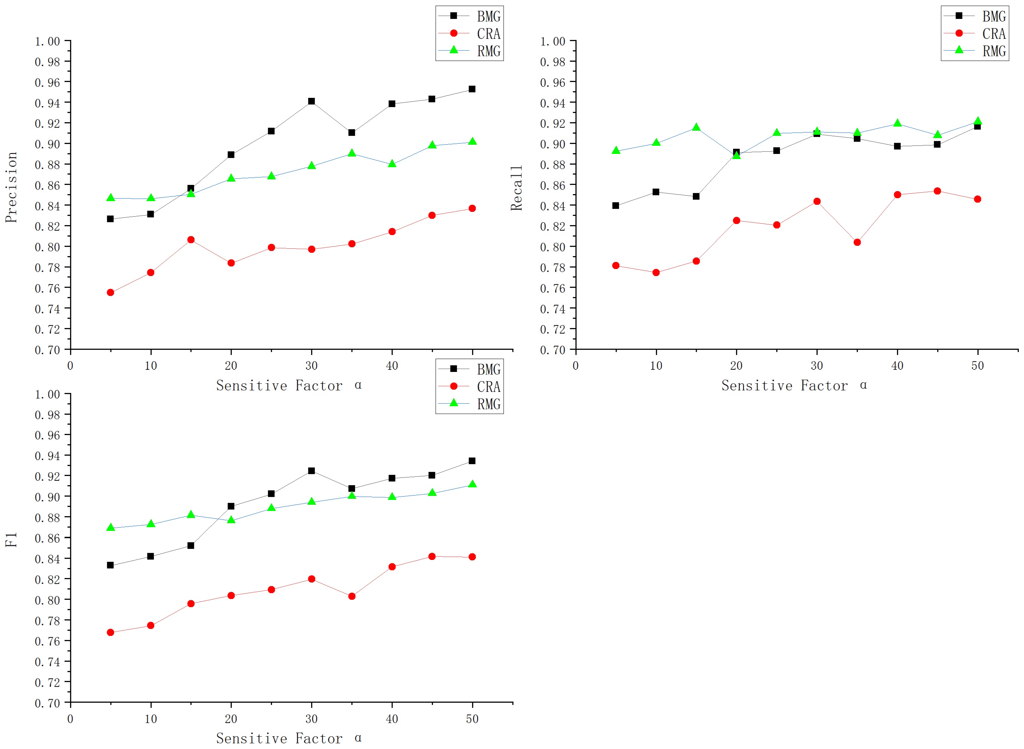
4.5.2. Impact of Different Cost-Sensitive Factor $\alpha$

To further demonstrate the contribution of the cost matrix to the classification performance of the minority classes, this experiment was conducted to verify its effect on the final experimental results by changing the value of the cost-sensitive factor $\alpha$. In the previous content, a relationship was established between High, Medium, and Low in the cost matrix, i.e., High = α ∗ α ∗ Low = α ∗ Medium. Keeping Low constant, as $\alpha$ increases, the corresponding cost increases, and the increase in the cost of misclassification is greater for the minority classes. Figure 6 shows the changes in F1-score, Recall, and Precision for BMG, CRA, and RMG with different cost-sensitive factor $\alpha$.

It may be observed from the results that, in terms of the F1-score, in general, the F1-score of the BMG class was the largest, because the cost associated with the BMG class was the largest, which compensated for the shortcoming of the BMG samples being the fewest. Although the cost-sensitive factor associated with the RMG class was the smallest Low, the maximum number of RMG samples made up for the low-cost factor and the F1-score of the RMG class was the second. The F1-score of the CRA class was the smallest because the sensitive factors related to CRA were not the largest and the number of CRA samples was small.

In terms of Precision, the Precision for the BMG class was the largest, the Precision for the RMG class was the second largest, and the Precision for the CRA class was the smallest. This result is consistent with that described in the previous paragraph. BMG exhibited a high misclassification cost and RMG had the most sample data; thus, the Precision for both was high, whereas CRA had fewer sample data and no high misclassification cost to compensate for the small number of samples; thus, the Precision was the smallest.

In terms of Recall, the Recall for the RMG class was the largest, the Recall for the BMG class was the second largest, and the Recall for the CRA class was the smallest. Precision and Recall are usually a pair of relative contradictory measures. When the Precision ratio is high, the Recall ratio tends to be low, and vice versa. Therefore, in this experiment, the F1-score and Precision for BMG were the highest, and its Recall became smaller accordingly.

From the perspective of change trend, with an increase in the cost-sensitive factor $\alpha$, all types of F1-score, Recall, and Precision showed an upward trend, indicating that the cost-sensitive matrix plays a positive role in the algorithm. As a result of the higher misclassification cost of samples in BMG and CRA, they were more affected by cost-sensitive factor $\alpha$, and the change trend of the three indicators in BMG and CRA was greater than that of the three indicators in RMG. With the increase in the cost-sensitive factor $\alpha$, the F1-score, Precision, and Recall for BMG increased from less than that for RMG to greater than that for RMG.

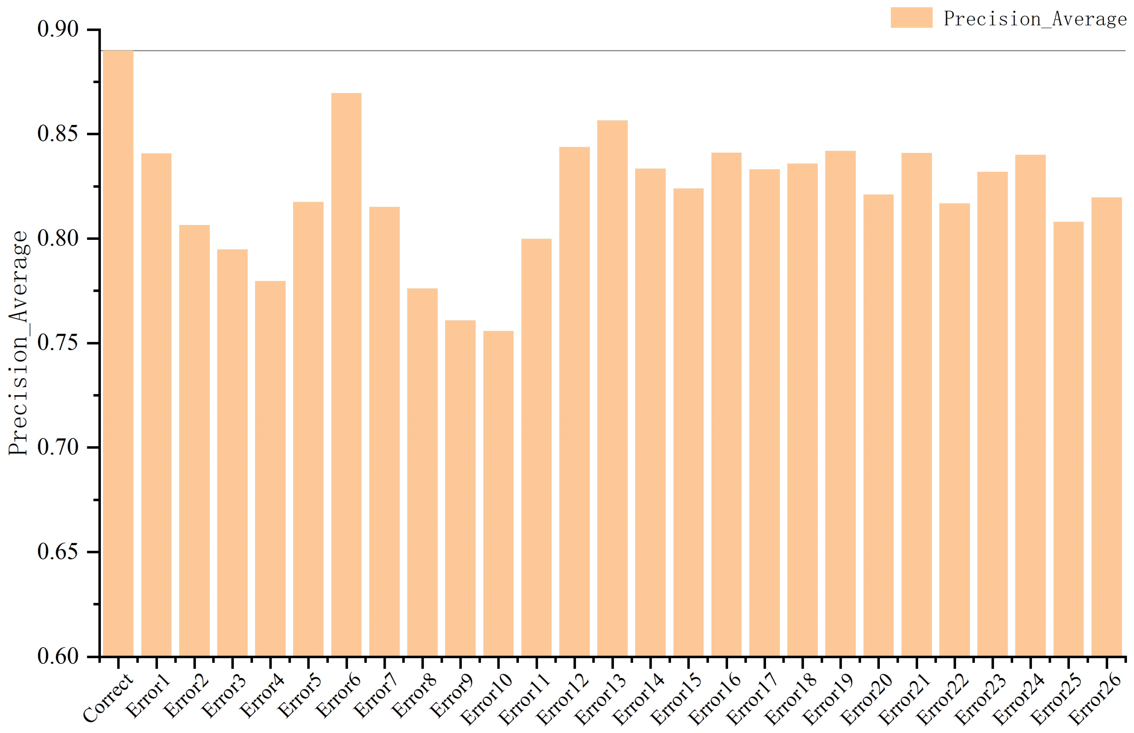
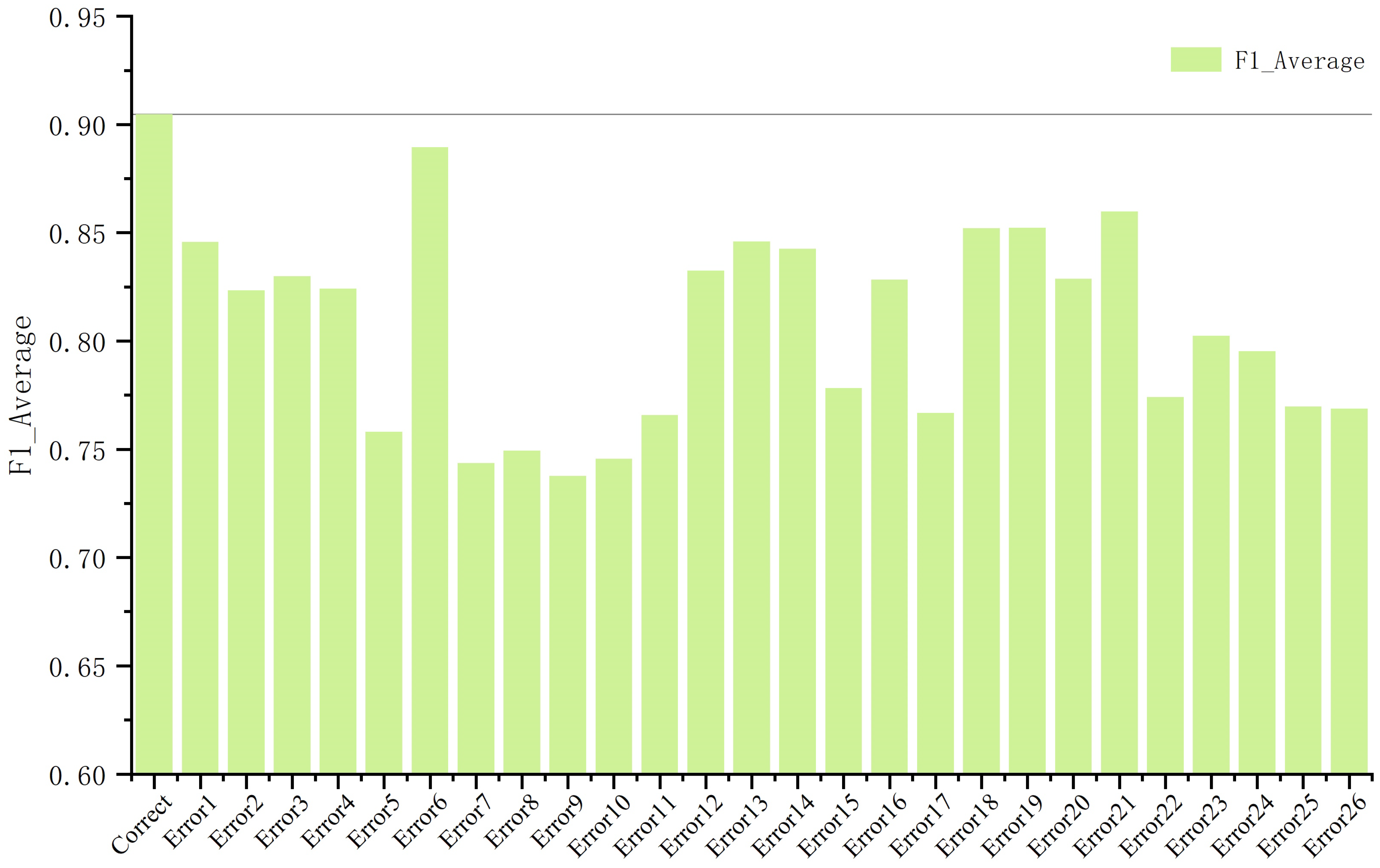
4.5.3. Influence of Cost Matrix of Correct Domain Knowledge Embedding on F1-score

To verify whether the correct sensitivity factors (High, Medium, and Low, which follow High > Medium > Low) would have a more positive impact on the experimental results, we tested the experimental results when the cost matrix was correct, and when the cost matrix was not in accordance with the reality. There were 27 possible scenarios of the cost matrix; all scenarios of the cost matrix are presented in

Table A1. Different cost matrix configurations. Here, there is one correct configuration from domain knowledge (Correct), and the other 26 (Error1–Error26) are not correct. H: High, M: Medium, L: Low.

	Correct			Error1			Error2
	BMG	CRA	RMG	BMG	CRA	RMG	BMG	CRA	RMG
BMG	1	H	H	1	H	H	1	H	H
CRA	M	1	M	M	1	M	M	1	M
RMG	L	L	1	M	M	1	H	H	1
	Error3			Error4			Error5
	BMG	CRA	RMG	BMG	CRA	RMG	BMG	CRA	RMG
BMG	1	H	H	1	H	H	1	H	H
CRA	L	1	L	L	1	L	L	1	L
RMG	L	L	1	M	M	1	H	H	1
	Error6			Error7			Error8
	BMG	CRA	RMG	BMG	CRA	RMG	BMG	CRA	RMG
BMG	1	H	H	1	H	H	1	H	H
CRA	H	1	H	H	1	H	H	1	H
RMG	L	L	1	M	M	1	H	H	1
	Error9			Error10			Error11
	BMG	CRA	RMG	BMG	CRA	RMG	BMG	CRA	RMG
BMG	1	L	L	1	L	L	1	L	L
CRA	M	1	M	M	1	M	M	1	M
RMG	L	L	1	M	M	1	H	H	1
	Error12			Error13			Error14
	BMG	CRA	RMG	BMG	CRA	RMG	BMG	CRA	RMG
BMG	1	L	L	1	L	L	1	L	L
CRA	L	1	L	L	1	L	L	1	L
RMG	L	L	1	M	M	1	H	H	1
	Error15			Error16			Error17
	BMG	CRA	RMG	BMG	CRA	RMG	BMG	CRA	RMG
BMG	1	L	L	1	L	L	1	L	L
CRA	H	1	H	H	1	H	H	1	H
RMG	L	L	1	M	M	1	H	H	1
	Error18			Error19			Error20
	BMG	CRA	RMG	BMG	CRA	RMG	BMG	CRA	RMG
BMG	1	M	M	1	M	M	1	M	M
CRA	M	1	M	M	1	M	M	1	M
RMG	L	L	1	M	M	1	H	H	1
	Error21			Error22			Error23
	BMG	CRA	RMG	BMG	CRA	RMG	BMG	CRA	RMG
BMG	1	M	M	1	M	M	1	M	M
CRA	L	1	L	L	1	L	L	1	L
RMG	L	L	1	M	M	1	H	H	1
	Error24			Error25			Error26
	BMG	CRA	RMG	BMG	CRA	RMG	BMG	CRA	RMG
BMG	1	M	M	1	M	M	1	M	M
CRA	H	1	H	H	1	H	H	1	H
RMG	L	L	1	M	M	1	H	H	1

of Appendix B and five typical scenarios of them are listed in

Table 5. Different cost matrix configurations. Here, there is one correct configuration from domain knowledge, and the other five (Error1–Error5) were not correct. H: High, M: Medium, L: Low.

	Correct			Error1			Error2
	BMG	CRA	RMG	BMG	CRA	RMG	BMG	CRA	RMG
BMG	1	H	H	1	H	H	1	H	H
CRA	M	1	M	L	1	L	L	1	L
RMG	L	L	1	L	L	1	H	H	1
	Error3			Error4			None
	BMG	CRA	RMG	BMG	CRA	RMG	BMG	CRA	RMG
BMG	1	L	L	1	L	L	1	L	L
CRA	L	1	L	H	1	H	H	1	H
RMG	H	H	1	L	L	1	H	H	1

. The results of all experiments are shown in

Table A2. F1-score, Recall, and Precision of different cost matrices.

	Precision			Recall			F1-Score
	BMG	CRA	RMG	BMG	CRA	RMG	BMG	CRA	RMG
Correct	0.9409	0.8313	0.8976	0.9200	0.7809	0.9239	0.9303	0.8734	0.9106
Error1	0.8762	0.8214	0.8246	0.8178	0.6076	0.9245	0.8460	0.8196	0.8717
Error2	0.8616	0.7597	0.7982	0.8119	0.5316	0.9070	0.8360	0.7849	0.8491
Error3	0.8807	0.7221	0.7816	0.8533	0.4504	0.9091	0.8668	0.7823	0.8405
Error4	0.8810	0.6898	0.7681	0.8667	0.4040	0.9036	0.8738	0.7682	0.8304
Error5	0.9254	0.7745	0.7526	0.6252	0.4227	0.9401	0.7462	0.6919	0.8360
Error6	0.9106	0.8255	0.8725	0.9052	0.7133	0.9231	0.9079	0.8635	0.8971
Error7	0.8529	0.7946	0.7980	0.5926	0.6220	0.9153	0.6993	0.6789	0.8527
Error8	0.8878	0.6892	0.7514	0.6563	0.4330	0.9040	0.7547	0.6724	0.8207
Error9	0.8424	0.6949	0.7453	0.6415	0.4124	0.9045	0.7283	0.6671	0.8173
Error10	0.8218	0.6944	0.7511	0.6696	0.4304	0.8959	0.7380	0.6818	0.8171
Error11	0.9106	0.7360	0.7531	0.6637	0.4149	0.9277	0.7678	0.6980	0.8313
Error12	0.9200	0.7787	0.8325	0.7837	0.6553	0.9102	0.8464	0.7812	0.8696
Error13	0.9492	0.7830	0.8372	0.8030	0.6579	0.9167	0.8700	0.7928	0.8751
Error14	0.8740	0.8015	0.8248	0.8222	0.6089	0.9167	0.8473	0.8117	0.8683
Error15	0.8523	0.7863	0.8331	0.6667	0.7113	0.8994	0.7481	0.7216	0.8650
Error16	0.8985	0.7919	0.8328	0.7733	0.6572	0.9132	0.8312	0.7825	0.8711
Error17	0.9062	0.7821	0.8108	0.6296	0.6476	0.9142	0.7430	0.6976	0.8594
Error18	0.8827	0.8005	0.8240	0.8474	0.5969	0.9177	0.8647	0.8233	0.8683
Error19	0.8894	0.8265	0.8099	0.8341	0.5738	0.9293	0.8609	0.8303	0.8655
Error20	0.9161	0.7519	0.7954	0.8089	0.5481	0.9078	0.8592	0.7793	0.8479
Error21	0.8741	0.8066	0.8418	0.8637	0.6450	0.9142	0.8689	0.8342	0.8765
Error22	0.8752	0.7698	0.8053	0.6652	0.6205	0.9059	0.7559	0.7137	0.8526
Error23	0.8796	0.8003	0.8158	0.7141	0.6250	0.9186	0.7882	0.7547	0.8641
Error24	0.8736	0.8302	0.8163	0.6859	0.6598	0.9229	0.7685	0.7512	0.8663
Error25	0.8602	0.7583	0.8054	0.6652	0.6209	0.8997	0.7502	0.7087	0.8499
Error26	0.8404	0.7905	0.8283	0.6474	0.7049	0.9005	0.7314	0.7118	0.8629

of Appendix C, and

Table 6. F1-score, Recall, and Precision of different cost matrices.

	Precision			Recall			F1-Score
	BMG	CRA	RMG	BMG	CRA	RMG	BMG	CRA	RMG
Correct	0.9409	0.8313	0.8976	0.9200	0.7809	0.9239	0.9303	0.8734	0.9106
Error1	0.8807	0.7221	0.7816	0.8533	0.4504	0.9091	0.8668	0.7823	0.8405
Error2	0.9254	0.7745	0.7526	0.6252	0.4227	0.9401	0.7462	0.6919	0.8360
Error3	0.9106	0.7360	0.7531	0.6637	0.4149	0.9277	0.7678	0.6980	0.8313
Error4	0.8523	0.7863	0.8331	0.6667	0.7113	0.8994	0.7481	0.7216	0.8650
Error5	0.9062	0.7821	0.8108	0.6296	0.6476	0.9142	0.7430	0.6976	0.8594

lists the six typical scenarios of them. The Precision, Recall, and F1-score of the result are shown in Figure A1, Figure A2 and Figure A3 of Appendix A more clearly.

It may be observed from the experimental results that, when the cost matrix was not embedded with domain knowledge, the F1-score, Recall, and Precision of the three types were reduced, which means that the embedding of domain knowledge into the cost matrix was effective.

Comparing the results of Error2 and Correct, the cost of CRA in Error1 was set to L and that of the other two were set to H; thus, the Recall, Precision, and F1-score for CRA in Error1 became smaller. Comparing the results of Error3 and Correct, Error3 set the cost of RMG as H and the cost of the other two as L, which was furthest from the actual domain knowledge; thus, the experimental result of this item was the worst. Comparing the results of Error5 and Correct, the cost of the BMG class in Error5 was set as L, and the cost of the other two categories was set as H; thus, the Recall and F1-score for BMG in Error1 became smaller.

5. Discussion and Future Work

Imbalanced data classification is concerned with the performance of learning algorithms in the presence of imbalanced data categories, and this problem has become a popular research topic in the field of machine learning. Traditional processing methods are based only on the data level or algorithm level for a single improvement. In this paper, we proposed a cost-sensitive VAE classifier method that combines the advantages of algorithm-level and data-level approaches.

-

To address the imbalance of data categories, this method incorporates a cost-sensitive factor so that the misclassification cost of minority-class samples is high and that of majority-class samples is low. Then, the overall misclassification cost is used as the model optimization target to improve the classification accuracy of the minority class. The results of Experiment 1 show that, in the task of amorphous alloy material classification, the cost-sensitive VAE outperforms other algorithms that favor a particular class of metrics in a comprehensive way. The F1-score, Precision, and Recall metrics are higher for each class of the data. Among them, the F1-score, Precision, and Recall for the minority classes (BMG) were 0.9432, 0.9644, and 0.9239, respectively.

-

Through Experiment 2, it was shown that the F1-score, Precision, and Recall of the three types of data classifications also increased for increasing values of the adjustment factor $\alpha$, indicating that the cost-sensitive factor has an effect on the classification of the imbalanced data. For the minority class, the three evaluation criteria grew faster.

-

The traditional method of designing the cost matrix is closely related to the number of samples, and generally takes the number of samples or the proportion of the number of samples as its cost, which cannot accurately reflect the real category distribution characteristics of the data. The proposed method combines the domain knowledge to design the cost matrix, and refines the cost-sensitive factor to make the cost matrix design more reasonable. The experimental results show that the method introducing correct domain knowledge results in a better F1-score, Precision, and Recall than other methods introducing wrong domain knowledge in the classification task of amorphous alloy materials. The results of Experiment 3 show that the algorithm introducing the cost matrix of correct domain knowledge exhibited a better F1-score, Precision, and Recall than the other five algorithms that introduced incorrect domain knowledge. The experimental results show that the correct cost matrix with domain knowledge can achieve a better classification effect, and that the embedding cost matrix with domain knowledge is effective.

Despite its performance, the cost-sensitive VAE has some limitations. The algorithm used in this study is a cost-sensitive variational classifier algorithm that incorporates the three cost sensitive parameters H, M, and L. In this study, we learned the size relationship of the three parameters through domain knowledge, so we introduced the adjustment factor $\alpha$ to set the corresponding equality relationship for the three parameters, and then determined the size of the three parameters through the grid search method. This method can be very time-consuming and labor-intensive when faced with the problem of having a very large search space.

Consequently, the following two points may be considered in future research.

-

Future studies can consider methods to learn the size of the three parameters H, M, and L through the algorithm adaptively; that is, methods designed to adaptively acquire domain knowledge adaptively.

-

In addition to the function of the cost-sensitive VAE classifier used in this study, the cost-sensitive VAE classifier can also generate new data by sampling the hidden variable Z and placing it into the decoder. Therefore, subsequent studies can also investigate how to compensate for the shortcomings of imbalanced datasets by generating new data.

References

1. Wu, X.; Kumar, V.; Quinlan, J.R.; Ghosh, J.; Yang, Q.; Motoda, H.; Mclachlan, G.J.; Ng, A.; Liu, B.; Yu, P.S.; et al. Top 10 algorithms in data mining. Knowl. Inf. Syst. 2008, 14, 1–37. [Google Scholar] [CrossRef] [Green Version]
2. Chawla, N.V.; Japkowicz, N.; Kotcz, A. Editorial: Special issue on learning from imbalanced data sets. SIGKDD Explor. 2004, 6, 1–6. [Google Scholar] [CrossRef]
3. Kubat, M.; Holte, R.C.; Matwin, S. Machine Learning for the Detection of Oil Spills in Satellite Radar Images. Mach. Learn. 1998, 30, 195–215. [Google Scholar] [CrossRef] [Green Version]
4. He, H.; Garcia, E.A. Learning from Imbalanced Data. IEEE Trans. Knowl. Data Eng. 2009, 21, 1263–1284. [Google Scholar]
5. Provost, F.J.; Weiss, G.M. Learning When Training Data are Costly: The Effect of Class Distribution on Tree Induction. arXiv 2011, arXiv:1106.4557. [Google Scholar]
6. Chawla, N.; Japkowic, N.; Kotcz, A.; Japkowicz, N. Editorial: Special issues on learning from imbalanced data sets. Ann. Nucl. Energy 2004, 36, 255–257. [Google Scholar] [CrossRef]
7. Chawla, N.V.; Bowyer, K.W.; Hall, L.O.; Kegelmeyer, W.P. SMOTE: Synthetic Minority Over-sampling Technique. J. Artif. Intell. Res. 2002, 16, 321–357. [Google Scholar] [CrossRef]
8. Han, H.; Wang, W.; Mao, B. Borderline-SMOTE: A New Over-Sampling Method in Imbalanced Data Sets Learning. In Advances in Intelligent Computing, Proceedings of the International Conference on Intelligent Computing, ICIC 2005, Hefei, China, 23–26 August 2005; Springer: Berlin/Heidelberg, Germany, 2005; pp. 878–887, Part I. [Google Scholar]
9. Zhu, T.; Lin, Y.; Liu, Y. Synthetic minority oversampling technique for multiclass imbalance problems. Pattern Recognit. 2017, 72, 327–340. [Google Scholar] [CrossRef]
10. Czarnowski, I. Learning from Imbalanced Data Using Over-Sampling and the Firefly Algorithm. In Proceedings of the Computational Collective Intelligence—13th International Conference, ICCCI 2021, Rhodes, Greece, 29 September–1 October 2021. [Google Scholar]
11. Czarnowski, I. Learning from Imbalanced Data Streams Based on Over-Sampling and Instance Selection. In Proceedings of the Computational Science—ICCS 2021—21st International Conference, Krakow, Poland, 16–18 June 2021. Part III. [Google Scholar]
12. Mayabadi, S.; Saadatfar, H. Two density-based sampling approaches for imbalanced and overlapping data. Knowl. Based Syst. 2022, 241, 108217. [Google Scholar] [CrossRef]
13. Weiss, G.M. Mining with rarity. ACM SIGKDD Explor. Newsl. 2004, 6, 7–19. [Google Scholar] [CrossRef]
14. Kubat, M.; Matwin, S. Addressing the Curse of Imbalanced Training Sets: One-Sided Selection. In Proceedings of the Fourteenth International Conference on Machine Learning (ICML 1997), Nashville, TN, USA, 8–12 July 1997. [Google Scholar]
15. Yen, S.J.; Lee, Y.S. Cluster-based under-sampling approaches for imbalanced data distributions. Expert Syst. Appl. 2009, 36, 5718–5727. [Google Scholar] [CrossRef]
16. Du, S.; Chen, S. Weighted support vector machine for classification. In Proceedings of the IEEE International Conference on Systems, Man and Cybernetics, Waikoloa, HI, USA, 10–12 October 2005. [Google Scholar]
17. Freund, Y. Boosting a Weak Learning Algorithm by Majority. Inf. Comput. 1995, 121, 256–285. [Google Scholar] [CrossRef]
18. Sahin, Y.; Bulkan, S.; Duman, E. A cost-sensitive decision tree approach for fraud detection. Expert Syst. Appl. 2013, 40, 5916–5923. [Google Scholar] [CrossRef]
19. Dhar, S.; Cherkassky, V. Development and Evaluation of Cost-Sensitive Universum-SVM. IEEE Trans. Cybern. 2015, 45, 806–818. [Google Scholar] [CrossRef] [PubMed]
20. Li, D.; Du, S.; Wu, T. A weighted support vector machine method and its application. J. Nat. Gas Sci. Eng. 2004, 2, 1834–1837. [Google Scholar]
21. Zhang, Z.; Luo, X.; García, S.; Herrera, F. Cost-Sensitive back-propagation neural networks with binarization techniques in addressing multi-class problems and non-competent classifiers. Appl. Soft Comput. 2017, 56, 357–367. [Google Scholar] [CrossRef]
22. Shen, W.; Wang, X.; Wang, Y.; Bai, X.; Zhang, Z. DeepContour: A Deep Convolutional Feature Learned by Positive-sharing Loss for Contour Detection. In Proceedings of the IEEE Conference on Computer Vision and Pattern Recognition, CVPR 2015, Boston, MA, USA, 7–12 June 2015. [Google Scholar]
23. Chung, Y.; Lin, H.; Yang, S. Cost-Aware Pre-Training for Multiclass Cost-Sensitive Deep Learning. In Proceedings of the Twenty-Fifth International Joint Conference on Artificial Intelligence, IJCAI 2016, New York, NY, USA, 9–15 July 2016. [Google Scholar]
24. Domingos, P.M. MetaCost: A General Method for Making Classifiers Cost-Sensitive. In Proceedings of the Fifth ACM SIGKDD International Conference on Knowledge Discovery and Data Mining, San Diego, CA, USA, 15–18 August 1999. [Google Scholar]
25. Madong, S. What Is the MetaCost. Available online: https://zhuanlan.zhihu.com/p/85527467 (accessed on 8 October 2019).
26. Galar, M.; Fernández, A.; Barrenechea, E.; Sola, H.; Herrera, F. A Review on Ensembles for the Class Imbalance Problem: Bagging-, Boosting-, and Hybrid-Based Approaches. Trans. Syst. Man Cybern. Part C Appl. Rev. 2012, 42, 463–484. [Google Scholar] [CrossRef]
27. Zhang, X.; Zhuang, Y.; Wang, W.; Pedrycz, W. Transfer Boosting with Synthetic Instances for Class Imbalanced Object Recognition. IEEE Trans. Cybern. 2018, 48, 357–370. [Google Scholar] [CrossRef]
28. Schapire, R.E. The strength of weak learnability. Proc. Second. Annu. Workshop Comput. Learn. Theory 1989, 5, 197–227. [Google Scholar]
29. Freund, Y.; Schapire, R.E. Experiments with a New Boosting Algorithm. In Machine Learning, Proceedings of the Thirteenth International Conference (ICML ’96), Bari, Italy, 3–6 July 1996; Lorenza Saitta: Bari, Italy, 1996; pp. 148–156. [Google Scholar]
30. Fan, W.; Stolfo, S.J.; Zhang, J.; Chan, P.K. AdaCost: Misclassification Cost-Sensitive Boosting. In Proceedings of the Sixteenth International Conference on Machine Learning (ICML 1999), Bled, Slovenia, 27–30 June 1999. [Google Scholar]
31. Sun, Y.; Kamel, M.S.; Wong, A.K.C.; Wang, Y. Cost-sensitive boosting for classification of imbalanced data. Pattern Recognit. 2007, 40, 3358–3378. [Google Scholar] [CrossRef]
32. Chawla, N.; Lazarevic, A.; Hall, L.; Bowyer, K. SMOTEBoost: Improving Prediction of the Minority Class in Boosting. In Proceedings of the 7th European Conference on Principles of Data Mining and Knowledge Discovery, Cavtat-Dubrovnik, Croatia, 22–26 September 2003; Springer: Berlin/Heidelberg, Germany, 2003. [Google Scholar]
33. Feng, W.; Huang, W.; Ren, J. Class Imbalance Ensemble Learning Based on the Margin Theory. Appl. Sci. 2018, 8, 815. [Google Scholar] [CrossRef] [Green Version]
34. Chen, S.; Shen, S.; Li, D. Imbalanced Data Integration learning method based on updating sample weight. Comput. Sci. 2018, 45, 31–37. [Google Scholar]
35. Kingma, D.P.; Welling, M. Auto-Encoding Variational Bayes. In Proceedings of the 2nd International Conference on Learning Representations, ICLR 2014, Banff, AB, Canada, 14–16 April 2014. [Google Scholar]
36. Dong, J.; Qian, Q. A Density-Based Random Forest for Imbalanced Data Classification. Future Internet 2022, 14, 90. [Google Scholar] [CrossRef]
Figure 1. The diagram of the proposed Cost-Sensitive Variational AutoEncoding Classifier algorithm. X denotes the original data, Z denotes the hidden variable, Z′ denotes the sample of Z, Y denotes the data label, and X′ denotes the reconstruction of the original data. The encoder module is used to obtain the distribution of hidden variable Z from the original data X, the decoder module is used to reconstruct samples and classify them, and the cost matrix module is used to adapt to imbalanced data.
Algorithms 15 00139 g001
Figure 2. Graph model of VAE.
Algorithms 15 00139 g002
Figure 3. Structure of the proposed variational autoencoder. The encoder accepts the input data X and outputs the distribution of the hidden variable. The decoder accepts the mean of the hidden variable Z and then outputs the reconstructed sample of the input data ( X ^ ). X and X ^ should be as close as possible.
Algorithms 15 00139 g003
Figure 4. Structure of the variational autoencoding classifier. Compared with the variational autoencoder, the variational autoencoding classifier includes a new output Y. X represents the input data, Y represents the label of the input data, and X ^ represents the reconstruction of the input data.
Algorithms 15 00139 g004
Figure 5. Structure of the cost-sensitive variational autoencoding classifier. Based on the variational autoencoding classifier, a cost-sensitive module is added to adapt to the imbalanced data. X represents the input data, Y represents the label of the input data, X ^ represents the reconstruction of the input data, and z represents hidden variable.
Algorithms 15 00139 g005
Figure 6. F1-score, Recall, and Precision under different cost sensitive factors α .
Algorithms 15 00139 g006