Adaptive Cooperative Control of Multiple Urban Rail Trains with Position Output Constraints

Abstract

This paper studies the distributed adaptive cooperative control of multiple urban rail trains with position output constraints and uncertain parameters. Based on an ordered set of trains running on the route, a dynamic multiple trains movement model is constructed to capture the dynamic evolution of the trains in actual operation. Aiming at the position constraints and uncertainties in the system, different distributed adaptive control algorithms are designed for all trains by using the local information about the position, speed and acceleration of the train operation, so that each train can dynamically adjust its speed through communicating with its neighboring trains. This control algorithm for each train is designed to track the desired position and speed curve, and the headway distance between any two neighboring trains is stable within a preset safety range, which guarantee the safety of tracking operation of multiple urban rail trains. Finally, the effectiveness of the designed scheme is verified by numerical examples.

1. Introduction

Under the condition that urban rail trains operate at high speed, high density, and long cycle automatic operation, effective train control strategies are needed to ensure the position and speed tracking accuracy of train operation. In order to solve these problems, many scholars have proposed different schemes. According to the number of controlled trains, the train control methods mainly include single train operation control and multiple trains cooperative control algorithms. The current control algorithms for single train mainly include PID control [1], fuzzy control [2], neural network control [3], adaptive control [4], predictive control [5], iterative learning [6], or the combination of several control theories [7,8,9], but in the environment of the high-density operation where interactions between trains are common, the control methods for single train can hardly meet the control requirements. However, the multiple trains cooperative control (MTCC) is applicable to train operation control in the case of mutual interference between trains. This method integrates the operating states of multiple trains and considers them as a whole for optimization, which is a solution to achieve global optimum and ensure system performance [10,11]. For example, the authors of [12] developed a multiple trains cooperative robust sampling data acquisition system to track the desired speed. The authors of [13] proposed a cooperative trains control method to reduce the energy consumption and peak demand of trains. The authors of [14,15] adopted a centralized control framework to design a MTCC strategy with the safe distance headway. However, the multiple trains cooperative method based on centralized control may reduce the robustness and reliability of the system and increase the computational complexity of the control system. To overcome these problems, the authors of [16] proposed a distributed MTCC based on nonlinear mapping feedback. The authors of [17] proposed an alternating direction method of multipliers to optimize the distributed control of multiple trains. Distributed control is able to equip each train with its own controller, allowing for more rational regulation of multiple trains movements, rather than relying on a centralized control mechanism that requires to observe and operate all trains. Therefore, distributed control is better for multiple trains cooperation system. In addition, since the actual train operation process is subject to various constraints, some researchers have studied the problem of distributed cooperative control with constraints. The authors of [18,19,20] investigated a multiple trains cooperative control method with saturation constraints. The authors of [21] proposed a multi-agent system with speed limit to improve the tracking accuracy of train operation control. The authors of [22] comprehensively studied distributed multi-agent systems with input control and non-convex velocity constraints. Previous literature on MTCC considers speed constraints and saturation constraints, but not position constraints. However, during the actual train operation and station stopping, the control system has strict requirements on the position output of the trains.

Inspired by these discussions, this paper focuses on the multiple trains distributed adaptive cooperative control scheme with position output constraints (POC) to track the desired train speed and position. Specifically, the main contributions of this paper are as follows.

• Considering the safety of multiple trains operation and station fixing stops, the distributed cooperative control law based on potential functions and POC is designed to ensure that each train tracks the desired train position and speed, at the same time, ensuring that the distance between each train and adjacent trains is within the predefined safety range.
• The adaptive laws automatically estimate the drag coefficient online, and proposes a single-value learning adaptive train cooperative control method to further simplify the structure of the controller.
• Different distributed control designs are applied to the various trains, not only for a single train, but also for a collection of $n$ trains ($n>1$ is a natural number). When the number of train groups varies, there exists no requirement to adjust the control structure or redesign the adaptive laws.

The rest of this paper is organized as follows. Section 2 introduces the multiple trains dynamic system model. Section 3 gives the detailed control schemes. Section 4 discusses the simulation results. Section 5 provides the concluding comments.

2. Preliminaries System Model

In the process of multiple trains tracking operation, each train is able to dynamically adjust its own speed based on communication with neighboring trains. In this paper, by treating each train as an agent and the information exchange between trains as the communication between agents, the tracking operation of the trains can be described by the framework of a multi-agent system.

Let $G=(V,E,A)$ be a weighted digraph of $n$ order, where $V=\left\{1,2,\cdots ,n\right\}$ is the set of nodes, $E\in V\times V$ is the set of edges, $A={\left[a_{ij}\right]}_{n\times n}$ is the nonnegative adjacency matrix of the digraph $G$, representing the information interaction between trains. If $(i,j)\in E$ holds, it means that the two trains can get the status data of each other, then $a_{ij}=1$, otherwise $a_{ij}=0$. $N_i=\left\{j\in V:\left(i,j\right)\in E\right\}$ represents the set of neighbors of node $i$. The Laplacian matrix $L$ corresponding to the adjacency matrix $A$ is described as ${\left[L\right]}_{ii}={\displaystyle \sum _{j=1,j\ne i}^n{a}_{ij}}$ and ${\left[L\right]}_{ij}=-a_{ij}$ for $i\ne j$.

For the MTCC system, this paper sets that each train can communicate with its neighboring trains, then the middle train can exchange data with its preceding and following trains. The foremost train can only communicate with the one immediately behind it, and the rearmost train can only communicate with the train immediately in front of it. So, the following adjacency matrix consisting of $n$ trains can be obtained as follows:

$$A=\left[\begin{array}{lllll}0\hfill & 1\hfill & 0\hfill & 0\hfill & \cdots \hfill \\ 1\hfill & 0\hfill & 1\hfill & 0\hfill & \cdots \hfill \\ ⋮\hfill & ⋮\hfill & ⋮\hfill & ⋮\hfill & ⋮\hfill \\ 0\hfill & \cdots \hfill & 1\hfill & 0\hfill & 1\hfill \\ 0\hfill & \cdots \hfill & 0\hfill & 1\hfill & 0\hfill \end{array}\right]$$

(1)

The corresponding Laplace matrix is expressed as follows:

$$L=\left[\begin{array}{lllll}1\hfill & -1\hfill & 0\hfill & 0\hfill & \cdots \hfill \\ -1\hfill & 2\hfill & -1\hfill & 0\hfill & \cdots \hfill \\ ⋮\hfill & ⋮\hfill & ⋮\hfill & ⋮\hfill & ⋮\hfill \\ 0\hfill & \cdots \hfill & -1\hfill & 2\hfill & -1\hfill \\ 0\hfill & \cdots \hfill & 0\hfill & -1\hfill & 1\hfill \end{array}\right]$$

(2)

In addition, in order to ensure that the safety separation distance between each train and its neighboring trains is stable within a certain range, the potential function is introduced in this paper as follows.

Definition 1.

$U_{i,j}(‖x_{i,j}‖)$ is a differentiable non-negative potential function of the distance $‖x_{i,j}‖$ between train $i$ and $j$, $l_1$ is the minimum safe separation distance between two neighboring trains, $l_2$ is the maximum allowable separation distance between two neighboring trains, and $l_1<l_2$, such that:

1. 

When$‖x_{i,j}‖\to l_1$or$‖x_{i,j}‖\to l_2$,$U_{i,j}(‖x_{i,j}‖)\to +\infty$;

2. 

When the positions of train$i$and$j$are at the desired position,$U_{i,j}(‖x_{i,j}‖)$is the unique minimum value.

Consider the cooperative operation system of multiple urban rail trains with n trains shown in Figure 1, the motion dynamics model of train $i$ can be described as follows:

$$\left\{\begin{array}{l}{\dot{x}}_{i,1}(t)=x_{i,2}(t)\hfill \\ {\dot{x}}_{i,2}(t)=u_i(t)-(a_{i,0}+a_{i,1}{x}_{i,2}(t)+a_{i,2}{x}_{i,2}^2(t))-(f_{i,s}+f_{i,c}+f_{i,t}),\hfill \end{array}\right.i=1,2,\cdots ,n$$

(3)

where $x_{i,1}(t)$ and $x_{i,2}(t)$ represent the position and speed of the $i$th train at time $t$, respectively, $u_i(t)$ is the cooperative control input to be designed, that is, the acceleration of the $i$th train, $a_{i,0}$, $a_{i,1}$, and $a_{i,2}$ are the basic operating resistance coefficients for the $i$th train, $f_{i,s}$ is the ramp resistance caused by the route slope, $f_{i,c}$ is the curve resistance caused by the route curve, and $f_{i,t}$ is the tunnel resistance caused by the route. During the actual train operation, the basic operating resistance coefficients $a_{i,0}$, $a_{i,1}$, $a_{i,2}$ and additional resistance $f_{i,s}$, $f_{i,c}$, $f_{i,t}$ change with different trains, weather conditions, outside environments, and other factors, these parameters are extremely difficult to get precisely, resulting in the parameters uncertainties of the train dynamics model. Among them, $\left|a_{i,0}\right|\le a_{i,0}^{+}$, $\left|a_{i,1}\right|\le a_{i,1}^{+}$, $\left|a_{i,2}\right|\le a_{i,2}^{+}$, $\left|f_{i,s}\right|\le f_{i,s}^{+}$, $\left|f_{i,c}\right|\le f_{i,c}^{+}$, and $\left|f_{i,t}\right|\le f_{i,t}^{+}$, $a_{i,0}^{+}$, $a_{i,1}^{+}$, $a_{i,2}^{+}$, $f_{i,s}^{+}$, $f_{i,c}^{+}$, and $f_{i,t}^{+}$ are the unknown upper bounds of the time-varying function, respectively. Thus, in this paper, an adaptive control scheme is designed to identify uncertain parameters to ensure the control performance of multiple trains cooperative control system.

Definition $f_i=a_{i,0}+f_{i,s}+f_{i,c}+f_{i,t}$, then the system model Equation (3) can be rewritten as follows:

$$\left\{\begin{array}{l}{\dot{x}}_{i,1}(t)=x_{i,2}(t)\hfill \\ {\dot{x}}_{i,2}(t)=u_i(t)-f_i-a_{i,1}{x}_{i,2}(t)-a_{i,2}{x}_{i,2}^2(t)\hfill \end{array}\right.$$

(4)

In order to ensure that the trains accurately track the operation curve and the requirements of station fixing stop in the MTCC operation system, the higher and lesser bounds of the train position output bounds need to be strictly restricted. It is defined as follows.

Lemma 1

([23]). For the train operation control system with position error ${\tilde{x}}_{i,1}$ and speed error ${\tilde{x}}_{i,2}$, there exist continuously differentiable and positive definite functions $V_{i,1}$ and $V_{i,2}$. The desired position outputs $x_{i,1d}$, and $k_i>0$ is the parameter limiting the value of the train position output. Define a position error of ${\tilde{x}}_{i,1}=x_{i,1}-x_{i,1d}$, such that

1. 

When${\tilde{x}}_{i,1}\to -k_i$or${\tilde{x}}_{i,1}\to k_i$,$V_{i,1}({\tilde{x}}_{i,1})\to +\infty$,

2. 

${\chi }_1(‖{\tilde{x}}_{i,2}‖)\le V_{i,2}({\tilde{x}}_{i,2})\le {\chi }_2(‖{\tilde{x}}_{i,2}‖)$, where${\chi }_1$and${\chi }_2$are$K_{\infty }$class functions.

Set $\left|{\tilde{x}}_{i,1}(0)\right|<k_i$, take $V_i=V_{i,1}({\tilde{x}}_{i,1})+V_{i,2}({\tilde{x}}_{i,2})$, if ${\dot{V}}_i\le 0$ can satisfy, then $\left|{\tilde{x}}_{i,1}(t)\right|<k_i$, $\forall t\in \left[0,\infty \right)$.

The design objectives of multiple trains distributed adaptive cooperative control are as follows.

• The position errors of all trains in the multiple trains cooperative operation are limited to a preset range, that is $\left|{\tilde{x}}_{i,1}(t)\right|<k_i$, and each train can accurately track the desired speed and distance curve.
• The separation distance between each train and neighboring trains in the MTCC system is kept within a predefined safety range.
• In the process of multiple trains tracking and cooperative operation, the speed of each train approaches the desired speed.

3. Control Law Design

In this section, two control schemes are proposed for multiple trains distributed adaptive cooperative control with POC and parameters uncertainties. The first is the multiple trains adaptive cooperative control with POC based on neighboring trains data, while the second is the multiple trains single-value learning adaptive cooperative control with POC. The second proposes a novel single-parameter adaptive control scheme, which requires only one online parameter adjustment and simplifies the structure of the controller.

3.1. Adaptive Cooperative Control Design of Multiple Trains with POC

For the MTCC system with POC and uncertain parameters, the distributed adaptive cooperative control algorithm based on the data of neighboring trains is designed as follows:

$$u_i(t)=u_{i,1}(t)+u_{i,2}(t)+u_{i,3}(t),\hspace{1em}i=1,2,\cdots ,n$$

(5)

$$u_{i,1}(t)={\widehat{f}}_i+{\widehat{a}}_{i,1}{x}_{i,2}+{\widehat{a}}_{i,2}{x}_{i,2}^2+{\dot{x}}_{i,2d}-{\beta }_i{\tilde{x}}_{i,2}-{\alpha }_i\frac{{\tilde{x}}_{i,1}}{k_i^2-{\tilde{x}}_{i,1}^2}$$

(6)

where ${\dot{\widehat{f}}}_i=-{\lambda }_{i,1}{\tilde{x}}_{i,2}(t)$, ${\dot{\widehat{a}}}_{i,1}=-{\lambda }_{i,2}{\tilde{x}}_{i,2}(t)x_{i,2}(t)$, and ${\dot{\widehat{a}}}_{i,2}=-{\lambda }_{i,3}{\tilde{x}}_{i,2}(t)x_{i,2}^2(t)$ are the parameter control laws, ${\lambda }_i\in \left\{{\lambda }_{i,1},{\lambda }_{i,2},{\lambda }_{i,3}\right\}$ is the positive design parameter, $x_{i,2d}$ is the desired speed output value, and ${\alpha }_i>0$ and ${\beta }_i>0$ are designed control gains.

Equation (6) is the position output constrained adaptive control part, which is used to identify the unknown parameters of the train model, compensate the desired speed, limit the position output, enable the train to accurately track the desired speed and distance curve, and achieve the first term of the control objective.

$u_{i,2}(t)$ is used to maintain the safe separation distance between each train and neighboring trains, and the specific design is as follows:

$$u_{i,2}(t)=-d_i{\displaystyle \sum _{j\in N_i}{a}_{ij}}{\nabla }_{x_{i,1}}{U}_{i,j}$$

(7)

where $d_i>0$ is the control parameter.

Artificial potential field function $U_{i,j}(x_{i,j})$ is introduced according to Definition 1.

$$U_{i,j}(x_{i,j})=\frac{1}{{‖x_{i,j}‖}^2-l_1^2}+\frac{1}{l_2^2-{‖x_{i,j}‖}^2},\hspace{1em}{l}_1<‖x_{i,j}‖<l_2$$

(8)

where $x_{i,j}=x_{i,1}-x_{j,1}$, $l_1$ is the minimum safe separation distance between two neighboring trains, and $l_2$ is the maximum allowable separation distance between two neighboring trains.

Equation (8) can ensure that the separation distance between two neighboring trains is kept within the preset safety range of $\left(l_1,l_2\right)$, and the rear-end collision of two neighboring trains can be avoided.

Remark 1.

$u_{i,2}$is the negative gradient of the artificial potential field function$U_{i,j}(x_{i,j})$, and$u_{i,2}$acts on the MTCC system to bring down$U_{i,j}(x_{i,j})$. When$x_{i,j}=\sqrt{\frac{l_1^2+l_2^2}{2}}$, the gradient information of$U_{i,j}(x_{i,j})$is equal to zero, at this time$u_{i,2}=0$, that is, the stable separation distance between two neighboring trains is$x_{i,j}=\sqrt{\frac{l_1^2+l_2^2}{2}}$.

$u_{i,3}(t)$ requires the speed of each train to be consistent, and the specific design is as follows:

$$u_{i,3}(t)=h_i{\displaystyle \sum _{j\in N_i}{a}_{ij}}\left(x_{j,2}(t)-x_{i,2}(t)\right)$$

(9)

where $h_i>0$ is the control parameter.

Define position tracking error ${\tilde{x}}_{i,1}(t)=x_{i,1}(t)-x_{i,2d}t$ and speed tracking error ${\tilde{x}}_{i,2}(t)=x_{i,2}(t)-x_{i,2d}$, by applying $u_i(t)$ to each train $i$, Equation (4) can be rewritten as the following multiple trains error dynamics system.

$$\left\{\begin{array}{ll}{\dot{\tilde{x}}}_{i,1}(t)=& {\tilde{x}}_{i,2}(t)\\ {\dot{\tilde{x}}}_{i,2}(t)=& {\tilde{f}}_i+{\tilde{a}}_{i,1}{x}_{i,2}(t)+{\tilde{a}}_{i,2}{x}_{i,2}^2(t)-{\beta }_i{\tilde{x}}_{i,2}(t)-{\alpha }_i\frac{{\tilde{x}}_{i,1}(t)}{k_i^2-{\tilde{x}}_{i,1}^2(t)}\\ & -d_i{\displaystyle \sum _{j\in N_i}{a}_{ij}}{\nabla }_{{\tilde{x}}_{i,1}}{\tilde{U}}_{i,j}+h_i{\displaystyle \sum _{j\in N_i}{a}_{ij}}\left({\tilde{x}}_{j,2}(t)-{\tilde{x}}_{i,2}(t)\right)\end{array}\right.$$

(10)

where ${\tilde{f}}_i={\widehat{f}}_i-f_i$, ${\tilde{a}}_{i,1}={\widehat{a}}_{i,1}-a_{i,1}$ and ${\tilde{a}}_{i,2}={\widehat{a}}_{i,2}-a_{i,2}$ are the estimated error values, respectively, ${\tilde{U}}_{i,j}=U_{i,j}({\tilde{x}}_{i,j})$.

Theorem 1.

For a set of n urban rail trains system (4) operating on the same route, an adaptive cooperative controller (5) with POC is used, in which each train can track the target speed-distance curve during train operation, the separation distance between two neighboring trains is always kept within the safe range of $(l_1,l_2)$, and the speed of each train is able to reach the desired speed. That is, the closed-loop dynamic system satisfies the control objective.

Proof of Theorem 1.

The symmetrical Barrier Lyapunov function for the POC is chosen as follows:

$$V_{i,1}({\tilde{x}}_{i,1})=\frac{1}{2}{\alpha }_i{\displaystyle \sum _{i=1}^n\log \frac{k_i^2}{k_i^2-{\tilde{x}}_{i,1}^2}}$$

(11)

According to Lemma 1, for $k_i>0$, if $\left|{\tilde{x}}_{i,1}(0)\right|<k_i$ holds, $\forall t\in \left[0,\infty \right)$, thus [23,24]

$$\log \frac{k_i^2}{k_i^2-{\tilde{x}}_{i,1}^2}<\frac{{\tilde{x}}_{i,1}^2}{k_i^2-{\tilde{x}}_{i,1}^2}$$

(12)

The differential of $V_{i,1}$ is obtained as follows:

$${\dot{V}}_{i,1}<{\alpha }_i{\displaystyle \sum _{i=1}^n\frac{{\tilde{x}}_{i,1}{\dot{\tilde{x}}}_{i,1}}{k_i^2-{\tilde{x}}_{i,1}^2}}={\alpha }_i{\displaystyle \sum _{i=1}^n\frac{{\tilde{x}}_{i,1}{\tilde{x}}_{i,2}}{k_i^2-{\tilde{x}}_{i,1}^2}}$$

(13)

The Lyapunov function is chosen as follows:

$$V_i=V_{i,1}+\frac{1}{2}{\displaystyle \sum _{i=1}^n{\tilde{x}}_{i,2}{\tilde{x}}_{i,2}}+\frac{1}{2}{\displaystyle \sum _{i=1}^n\left(\frac{{\tilde{f}}_{i,1}^2}{{\lambda }_{i,1}}+\frac{{\tilde{a}}_{i,2}^2}{{\lambda }_{i,2}}+\frac{{\tilde{a}}_{i,3}^2}{{\lambda }_{i,3}}\right)}$$

(14)

The differential of $V_i$ is obtained as follows:

$$\begin{array}{lll}{\dot{V}}_i& =& {\alpha }_i{\displaystyle \sum _{i=1}^n\frac{{\tilde{x}}_{i,1}{\tilde{x}}_{i,2}}{k_i^2-{\tilde{x}}_{i,1}^2}+}{\displaystyle \sum _{i=1}^n{\tilde{x}}_{i,2}{\dot{\tilde{x}}}_{i,2}}+{\displaystyle \sum _{i=1}^n\left(\frac{{\tilde{f}}_i{\dot{\tilde{f}}}_i}{{\lambda }_{i,1}}+\frac{{\tilde{a}}_{i,1}{\dot{\tilde{a}}}_{i,1}}{{\lambda }_{i,2}}+\frac{{\tilde{a}}_{i,2}{\dot{\tilde{a}}}_{i,2}}{{\lambda }_{i,3}}\right)}\\ & =& {\alpha }_i{\displaystyle \sum _{i=1}^n\frac{{\tilde{x}}_{i,1}{\tilde{x}}_{i,2}}{k_i^2-{\tilde{x}}_{i,1}^2}+}{\displaystyle \sum _{i=1}^n{\tilde{x}}_{i,2}\left[{\dot{x}}_{i,2}-{\dot{x}}_{i,2d}\right]}+{\displaystyle \sum _{i=1}^n\left(\frac{{\tilde{f}}_i{\dot{\tilde{f}}}_i}{{\lambda }_{i,1}}+\frac{{\tilde{a}}_{i,1}{\dot{\tilde{a}}}_{i,1}}{{\lambda }_{i,2}}+\frac{{\tilde{a}}_{i,2}{\dot{\tilde{a}}}_{i,2}}{{\lambda }_{i,3}}\right)}\\ & =& {\alpha }_i{\displaystyle \sum _{i=1}^n\frac{{\tilde{x}}_{i,1}{\tilde{x}}_{i,2}}{k_i^2-{\tilde{x}}_{i,1}^2}+{\displaystyle \sum _{i=1}^n{\tilde{x}}_{i,2}\left[{\tilde{f}}_i+{\tilde{a}}_{i,1}{x}_{i,2}+{\tilde{a}}_{i,2}{x}_{i,2}^2-{\beta }_i{\tilde{x}}_{i,2}-{\alpha }_i\frac{{\tilde{x}}_{i,1}}{k_i^2-{\tilde{x}}_{i,1}^2}\right]}}\\ & & -{\displaystyle \sum _{i=1}^n\left({\tilde{x}}_{i,2}{\tilde{f}}_i+{\tilde{x}}_{i,2}{\tilde{a}}_{i,1}{x}_{i,2}+{\tilde{x}}_{i,2}{\tilde{a}}_{i,2}{x}_{i,2}^2\right)}\\ & =& -{\beta }_i{\displaystyle \sum _{i=1}^n{\tilde{x}}_{i,2}^2}\end{array}$$

(15)

From ${\beta }_i>0$, we can know that ${\dot{V}}_i\le 0$. Then, ${\dot{V}}_i$ is semi-negative definite, so $V_i$ is a not-increasing state, and its numerical boundary value is $V_i(0)$, i.e., $V_i$ is bounded, which further ensures the boundedness of ${\tilde{x}}_{i,1}$, ${\tilde{x}}_{i,2}$, ${\tilde{f}}_i$, ${\tilde{a}}_{i,1}$, and ${\tilde{a}}_{i,2}$. Therefore, the control input $u_{i,1}$ is bounded. It is further guaranteed that ${\ddot{V}}_i$ is bounded by differentiating both sides of Equation (15), so ${\dot{V}}_i$ is consistently continuous. According to Barbǎlat Lemma, it is known that $\underset{t\to \infty }{\lim }{\dot{V}}_i(t)=0$. According to the linear control theory, it is known that the designed controller can guarantee the asymptotic speed and position tracking of each train, and achieve the tracking of the target speed-distance curve.

Based on the error dynamics Equation (10) for multiple trains operation, the following global positive definite Lyapunov function is selected as

$$Q_1=\frac{1}{2}{d}_i{\displaystyle \sum _{i=1}^n{\displaystyle \sum _{j=1}^n{a}_{ij}{\tilde{U}}_{i,j}}+\frac{1}{2}{\displaystyle \sum _{i=1}^n{\tilde{x}}_{i,2}{\tilde{x}}_{i,2}}}+\frac{1}{2}{\alpha }_i{\displaystyle \sum _{i=1}^n\log \frac{k_i^2}{k_i^2-{\tilde{x}}_{i,1}^2}}+\frac{1}{2}{\displaystyle \sum _{i=1}^n\left(\frac{{\tilde{f}}_{i,1}^2}{{\lambda }_{i,1}}+\frac{{\tilde{a}}_{i,2}^2}{{\lambda }_{i,2}}+\frac{{\tilde{a}}_{i,3}^2}{{\lambda }_{i,3}}\right)}$$

(16)

The differential of $Q_1$ is obtained as follows:

$$\begin{array}{ll}{\dot{Q}}_1=& \frac{1}{2}{d}_i{\displaystyle \sum _{i=1}^n{\displaystyle \sum _{j=1}^n{a}_{ij}{\dot{\tilde{U}}}_{i,j}}}+{\displaystyle \sum _{i=1}^n{\tilde{x}}_{i,2}}\left[-d_i{\displaystyle \sum _{j\in N_i}{a}_{ij}}{\nabla }_{{\tilde{x}}_{i,1}}{\tilde{U}}_{i,j}+h_i{\displaystyle \sum _{j\in N_i}{a}_{ij}}\left({\tilde{x}}_{j,2}-{\tilde{x}}_{i,2}\right)\right]\hfill \\ & +{\displaystyle \sum _{i=1}^n{\tilde{x}}_{i,2}}\left[{\tilde{f}}_i+{\tilde{a}}_{i,1}{x}_{i,2}+{\tilde{a}}_{i,2}{x}_{i,2}^2-{\beta }_i{\tilde{x}}_{i,2}-{\alpha }_i\frac{{\tilde{x}}_{i,1}}{k_i^2-{\tilde{x}}_{i,1}^2}\right]\hfill \\ \\ & +{\alpha }_i{\displaystyle \sum _{i=1}^n\frac{{\tilde{x}}_{i,1}{\tilde{x}}_{i,2}}{k_i^2-{\tilde{x}}_{i,1}^2}}+{\displaystyle \sum _{i=1}^n\left(\frac{{\tilde{f}}_i{\dot{\tilde{f}}}_i}{{\lambda }_{i,1}}+\frac{{\tilde{a}}_{i,1}{\dot{\tilde{a}}}_{i,1}}{{\lambda }_{i,2}}+\frac{{\tilde{a}}_{i,2}{\dot{\tilde{a}}}_{i,2}}{{\lambda }_{i,3}}\right)}\hfill \end{array}$$

(17)

Sort out the first item in Equation (17), and we get that

$$\begin{array}{ll}\frac{1}{2}{d}_i{\displaystyle \sum _{i=1}^n{\displaystyle \sum _{j=1}^n{a}_{ij}{\dot{\tilde{U}}}_{i,j}}}& =\frac{1}{2}{d}_i{\displaystyle \sum _{i=1}^n{\displaystyle \sum _{j=1}^n{a}_{ij}{\nabla }_{{\tilde{x}}_{i,j}}{\tilde{U}}_{i,j}{\dot{\tilde{x}}}_{i,j}}}\hfill \\ & =\frac{1}{2}{d}_i{\displaystyle \sum _{i=1}^n{\displaystyle \sum _{j=1}^n{a}_{ij}{\nabla }_{{\tilde{x}}_{i,j}}{\tilde{U}}_{i,j}}}({\dot{\tilde{x}}}_{i,1}-{\dot{\tilde{x}}}_{j,1})\\ & =\frac{1}{2}{d}_i{\displaystyle \sum _{i=1}^n{\displaystyle \sum _{j=1}^n{a}_{ij}\left({\tilde{x}}_{i,2}{\nabla }_{{\tilde{x}}_{i,1}}+{\tilde{x}}_{j,2}{\nabla }_{{\tilde{x}}_{j,1}}\right){\tilde{U}}_{i,j}}}\\ & =d_i{\displaystyle \sum _{i=1}^n{\displaystyle \sum _{j=1}^n{a}_{ij}{\tilde{x}}_{i,2}{\nabla }_{{\tilde{x}}_{i,1}}{\tilde{U}}_{i,j}}}\end{array}$$

(18)

The Equation (17) can be expressed as

$$\begin{array}{ll}{\dot{Q}}_1=& h_i{\displaystyle \sum _{i=1}^n{\tilde{x}}_{i,2}}\left[{\displaystyle \sum _{j\in N_i}{a}_{ij}}({\tilde{x}}_{j,2}-{\tilde{x}}_{i,2})\right]\\ & +{\displaystyle \sum _{i=1}^n{\tilde{x}}_{i,2}}\left({\tilde{f}}_i+{\tilde{a}}_{i,1}{x}_{i,2}+{\tilde{a}}_{i,2}{x}_{i,2}^2-{\beta }_i{\tilde{x}}_{i,2}\right)\\ & +{\displaystyle \sum _{i=1}^n\left(-{\tilde{x}}_{i,2}{\tilde{f}}_i-{\tilde{x}}_{i,2{\tilde{a}}_{i,1}}{x}_{i,2}-{\tilde{x}}_{i,2}{\tilde{a}}_{i,2}{x}_{i,2}^2\right)}\\ & =-h_i{\tilde{x}}_2^{\mathrm{T}}L{\tilde{x}}_2-{\beta }_i{\tilde{x}}_2^{\mathrm{T}}{\tilde{x}}_2\end{array}$$

(19)

where ${\tilde{x}}_2={\left({\tilde{x}}_{1,2},{\tilde{x}}_{2,2},\cdots ,{\tilde{x}}_{n,2}\right)}^{\mathrm{T}}$.

From Laplace matrices $L\ge 0$, $h_i>0$ and ${\beta }_i>0$, we know that ${\dot{Q}}_1\le 0$.

Integrate Equation (19) from 0 to t yields, $Q_1(t)-Q_1(0)\le 0$. Therefore, for any time $t\ge 0$, $Q_1$ is bounded. Equation (16) implies that for any $(i,j)\in E$, ${\tilde{U}}_{i,j}\le Q_1(t)\le Q_1(0)$, i.e., ${\tilde{U}}_{i,j}$ is bounded. However, for some $i,j\in E$, if $x_{i,j}\to l_1$ or $x_{i,j}\to l_2$, then ${\tilde{U}}_{i,j}\to \infty$. Thus, if ${\tilde{U}}_{i,j}$ wants to satisfy the continuity and boundedness, for any $t\ge 0$, $l_1\le \left|x_{i,j}\right|\le l_2$, that is, the separation distance between the neighboring trains should be kept within the safety range of $(l_1,l_2)$. Therefore, the certain safety separation distance can be maintained between two neighboring trains to ensure the safety of multiple trains operation.

Furthermore, according to Equation (19), it is known that if ${\tilde{x}}_2(t)=0$, then ${\dot{Q}}_1(t)=0$. Therefore, for the error system of Equation (10), the set $\Omega \left\{\left({\tilde{x}}_{i,1}(t),{\tilde{x}}_{i,2}(t)\left|{\tilde{x}}_{i,2}(t)=0\right.\right)\right\}$ is the largest invariant set contained in $\mathrm{B}=\left\{\left({\tilde{x}}_{i,1}(t),{\tilde{x}}_{i,2}(t)\left|{\dot{Q}}_1(t)=0\right.\right)\right\}$. According to the LaSalles invariance principle, each solution of the Equation (10) beginning from any original situation converges to the maximal invariant set in $\left\{\left({\tilde{x}}_{i,1}(t),{\tilde{x}}_{i,2}(t)\left|{\dot{Q}}_1(t)=0\right.\right)\right\}$. Since ${\dot{Q}}_1(t)=0$ implies that ${\tilde{x}}_{i,2}(t)=0$, i.e., $x_{1,2}=x_{2,2}=\cdots =x_{n,2}=x_{i,2d}$. Therefore, the speed of each train reaches the desired speed $x_{i,2d}$. □

3.2. Single-Value Learning Adaptive Cooperative Control Design of Multiple Trains with POC

In order to simplify the structure of the controller, this subsection proposes a novel single-parameter adaptive control method. By selecting a new type of parameter to be estimated, only one online parameter adjustment is required, which effectively improves the engineering practicability of the controller.

Based on the data of neighboring trains, the adaptive cooperative control law for multiple urban rail trains is designed as follows:

$$\begin{array}{ll}{u}_i=& -{\widehat{\Theta }}_i{\psi }^2(x_{i,2}){\tilde{x}}_{i,2}+{\dot{x}}_{i,2d}-{\alpha }_i\frac{{\tilde{x}}_{i,1}}{k_i^2-{\tilde{x}}_{i,1}^2}\hfill \\ & -d_i{\displaystyle \sum _{j\in N_i}{a}_{ij}}{\nabla }_{x_{i,1}}{U}_{i,j}+h_i{\displaystyle \sum _{j\in N_i}{a}_{ij}}\left(x_{j,2}-x_{i,2}\right)\hfill \end{array}$$

(20)

where $\psi (x_{i,2})=1+x_{i,2}+x_{i,2}^2$, ${\Theta }_i=\max \left\{f_i,a_{i,1},a_{i,2}\right\}$, ${\widehat{\Theta }}_i$ is the estimated value of ${\Theta }_i$, the adaptive law of ${\widehat{\Theta }}_i$ is designed as follows:

$${\dot{\widehat{\Theta }}}_i={\theta }_i{\psi }^2(x_{i,2}){\tilde{x}}_{i,2}^2$$

(21)

where ${\theta }_i>0$ is the control parameter.

Theorem 2.

For an ordered collection of n trains, the distributed controller in Equation (20) and the adaptive law in Equation (21) are designed so that each train can track the target speed-distance curve, the separation distance between two neighboring trains is always kept within the safe range of $(l_1,l_2)$, and the speed of each train can reach the desired speed. That is, the closed-loop dynamic system satisfies the control objective.

Proof of Theorem 2.

Define the parameter estimation error ${\tilde{\Theta }}_i={\widehat{\Theta }}_i-{\Theta }_i$, based on the coordinates ${\tilde{x}}_{i,1}$, ${\tilde{x}}_{i,2}$, ${\tilde{x}}_{j,2}$, ${\tilde{\Theta }}_i$, and ${\tilde{U}}_{i,j}$, the dynamics of the multiple trains closed-loop system can be obtained as follows:

$$\left\{\begin{array}{l}{\dot{\tilde{x}}}_{i,1}={\tilde{x}}_{i,2}\\ {\dot{\tilde{x}}}_{i,2}=-{\tilde{\Theta }}_i{\psi }^2(x_{i,2}){\tilde{x}}_{i,2}-{\alpha }_i\frac{{\tilde{x}}_{i,1}}{k_i^2-{\tilde{x}}_{i,1}^2}-d_i{\displaystyle \sum _{j\in N_i}{a}_{ij}}{\nabla }_{{\tilde{x}}_{i,1}}{\tilde{U}}_{i,j}+h_i{\displaystyle \sum _{j\in N_i}{a}_{ij}}\left({\tilde{x}}_{j,2}-{\tilde{x}}_{i,2}\right)\\ {\dot{\tilde{\Theta }}}_i={\theta }_i{\psi }^2(x_{i,2}){\tilde{x}}_{i,2}^2\end{array}\right.$$

(22)

The following global positive definite Lyapunov function is selected so that

$$Q_2=\frac{1}{2}{d}_i{\displaystyle \sum _{i=1}^n{\displaystyle \sum _{j=1}^n{a}_{ij}{\tilde{U}}_{i,j}}+\frac{1}{2}{\displaystyle \sum _{i=1}^n{\tilde{x}}_{i,2}{\tilde{x}}_{i,2}}}+\frac{1}{2}{\alpha }_i{\displaystyle \sum _{i=1}^n\log \frac{k_i^2}{k_i^2-{\tilde{x}}_{i,1}^2}}+\frac{1}{2}{\displaystyle \sum _{i=1}^n\frac{{\tilde{\Theta }}_i^2}{{\theta }_i}}$$

(23)

The differential of $Q_2$ is obtained as follows:

$$\begin{array}{ccc}\hfill {\dot{Q}}_2& =& \frac{1}{2}{d}_i{\displaystyle \sum _{i=1}^n{\displaystyle \sum _{j=1}^n{a}_{ij}{\dot{\tilde{U}}}_{i,j}}}+{\displaystyle \sum _{i=1}^n{\tilde{x}}_{i,2}}\left[-{\widehat{\Theta }}_i{\psi }^2(x_{i,2}){\tilde{x}}_{i,2}-{\alpha }_i\frac{{\tilde{x}}_{i,1}}{k_i^2-{\tilde{x}}_{i,1}^2}\right]\hfill \\ & & -{\displaystyle \sum _{i=1}^n{\tilde{x}}_{i,2}}\left[f_i+a_{i,1}{x}_{i,2}+a_{i,2}{x}_{i,2}^2\right]+{\displaystyle \sum _{i=1}^n{\tilde{x}}_{i,2}}\left[-d_i{\displaystyle \sum _{j\in N_i}{a}_{ij}}{\nabla }_{{\tilde{x}}_{i,1}}{\tilde{U}}_{ij}+h_i{\displaystyle \sum _{j\in N_i}{a}_{ij}}\left({\tilde{x}}_{j,2}-{\tilde{x}}_{i,2}\right)\right]\hfill \\ & & +{\alpha }_i{\displaystyle \sum _{i=1}^n\frac{{\tilde{x}}_{i,1}{\tilde{x}}_{i,2}}{k_i^2-{\tilde{x}}_{i,1}^2}}+{\displaystyle \sum _{i=1}^n\left(\frac{{\tilde{\Theta }}_i{\dot{\tilde{\Theta }}}_i}{{\theta }_i}\right)}\hfill \\ & \hfill \le & \frac{1}{2}{d}_i{\displaystyle \sum _{i=1}^n{\displaystyle \sum _{j=1}^n{a}_{ij}{\dot{\tilde{U}}}_{i,j}}}-{\widehat{\Theta }}_i{\displaystyle \sum _{i=1}^n{\psi }^2(x_{i,2}){\tilde{x}}_{i,2}^2}+{\Theta }_i{\displaystyle \sum _{i=1}^n{\tilde{x}}_{i,2}^2{(1+x_{i,2}+x_{i,2}^2)}^2}\hfill \\ & & +{\displaystyle \sum _{i=1}^n{\tilde{x}}_{i,2}}\left[-d_i{\displaystyle \sum _{j\in N_i}{a}_{ij}}{\nabla }_{{\tilde{x}}_{i,1}}{\tilde{U}}_{i,j}\right]+{\displaystyle \sum _{i=1}^n{\tilde{x}}_{i,2}}\left[h_i{\displaystyle \sum _{j\in N_i}{a}_{ij}}\left({\tilde{x}}_{j,2}-{\tilde{x}}_{i,2}\right)\right]\hfill \\ & & +{\displaystyle \sum _{i=1}^n\left(\frac{{\tilde{\Theta }}_i\left[{\theta }_i{\psi }^2(x_{i,2}){\tilde{x}}_{i,2}^2\right]}{{\theta }_i}\right)}\hfill \\ & \hfill =& \frac{1}{2}{d}_i{\displaystyle \sum _{i=1}^n{\displaystyle \sum _{j=1}^n{a}_{ij}{\dot{\tilde{U}}}_{i,j}}}-{\widehat{\Theta }}_i{\displaystyle \sum _{i=1}^n{\psi }^2(x_{i,2}){\tilde{x}}_{i,2}^2}+{\Theta }_i{\displaystyle \sum _{i=1}^n{\tilde{x}}_{i,2}^2{\psi }^2(x_{i,2})}\hfill \\ & & +{\displaystyle \sum _{i=1}^n{\tilde{x}}_{i,2}}\left[-d_i{\displaystyle \sum _{j\in N_i}{a}_{ij}}{\nabla }_{{\tilde{x}}_{i,1}}{\tilde{U}}_{i,j}\right]+{\displaystyle \sum _{i=1}^n{\tilde{x}}_{i,2}}\left[h_i{\displaystyle \sum _{j\in N_i}{a}_{ij}}\left({\tilde{x}}_{j,2}-{\tilde{x}}_{i,2}\right)\right]\hfill \\ & & +{\displaystyle \sum _{i=1}^n\left(\frac{{\tilde{\Theta }}_i\left[{\theta }_i{\psi }^2(x_{i,2}){\tilde{x}}_{i,2}^2\right]}{{\theta }_i}\right)}\hfill \end{array}$$

(24)

According to Equation (18) (${\displaystyle {\sum }_{i=1}^n{\displaystyle {\sum }_{j=1}^n{a}_{ij}{\dot{\tilde{U}}}_{i,j}}}=2{\displaystyle {\sum }_{i=1}^n{\displaystyle {\sum }_{j=1}^n{a}_{ij}{\tilde{x}}_{i,2}{\nabla }_{{\tilde{x}}_{i,1}}{\tilde{U}}_{i,j}}}$), Equation (24) is as follows:

$${\dot{Q}}_2=-h_i{\tilde{x}}_2^{\mathrm{T}}L{\tilde{x}}_2$$

(25)

where ${\tilde{x}}_2={\left({\tilde{x}}_{1,2},{\tilde{x}}_{2,2},\cdots ,{\tilde{x}}_{n,2}\right)}^{\mathrm{T}}$. The specific analysis process is similar to Section 3.1. From Laplace matrices $L\ge 0$ and $h_i>0$, we know that ${\dot{Q}}_2\le 0$. By integrating Equation (25) from 0 to t, we can get that $Q_2$ is bounded. Furthermore, from Equation (23) we know that ${\tilde{U}}_{i,j}$ is bounded. Thus, if ${\tilde{U}}_{i,j}$ wants to satisfy the continuity and boundedness, then for any $t\ge 0$, $l_1\le \left|x_{i,j}\right|\le l_2$; that is, the distance between two trains is kept within the safe range $(l_1,l_2)$. Therefore, the certain safety separation distance can be maintained between two neighboring trains to ensure the safety of multiple trains tracking operation.

Additionally, from Equation (25), it is known that if ${\tilde{x}}_2(t)=0$, then ${\dot{Q}}_2(t)=0$. Thus, for the error system of Equation (10), the set $\Omega \left\{\left({\tilde{x}}_{i,1}(t),{\tilde{x}}_{i,2}(t)\left|{\tilde{x}}_{i,2}(t)=0\right.\right)\right\}$ is the largest invariant set contained in the set $\mathrm{B}=\left\{\left({\tilde{x}}_{i,1}(t),{\tilde{x}}_{i,2}(t)\left|{\dot{Q}}_2(t)=0\right.\right)\right\}$. According to the LaSalles invariance principle, each solution beginning from any original situation converges to the maximal invariant set in $\left\{\left({\tilde{x}}_{i,1}(t),{\tilde{x}}_{i,2}(t)\left|{\dot{Q}}_2(t)=0\right.\right)\right\}$. Since ${\dot{Q}}_2(t)=0$ is established, it means that ${\tilde{x}}_{i,2}(t)=0$, i.e., $x_{1,2}=x_{2,2}=\cdots =x_{n,2}=x_{i,2d}$. Therefore, the speed of each train reaches the desired speed $x_{i,2d}$.

To enhance the robustness of the controller, based on the $\sigma$ modified robust adaptive control theory [25], the modified adaptive laws are as follows:

$${\dot{\widehat{f}}}_i=-{\lambda }_{i,1}\left({\tilde{x}}_{i,2}(t)+{\sigma }_{i,1}{\widehat{f}}_i\right)$$

(26)

$${\dot{\widehat{a}}}_{i,1}=-{\lambda }_{i,2}\left({\tilde{x}}_{i,2}(t)x_{i,2}(t)+{\sigma }_{i,2}{\widehat{a}}_{i,1}\right)$$

(27)

$${\dot{\widehat{a}}}_{i,2}=-{\lambda }_{i,3}\left({\tilde{x}}_{i,2}(t)x_{i,2}^2(t)+{\sigma }_{i,3}{\widehat{a}}_{i,2}\right)$$

(28)

$${\dot{\widehat{\Theta }}}_i={\theta }_i\left[{\psi }^2(x_{i,2}){\tilde{x}}_{i,2}^2-{\sigma }_{i,4}{\widehat{\Theta }}_i\right]$$

(29)

where ${\sigma }_i\in \left\{{\sigma }_{i,1},{\sigma }_{i,2},{\sigma }_{i,3},{\sigma }_{i,4}\right\}$ is a modified small positive constant. □

4. Simulation Results

In order to verify the effectiveness of the designed MTCC schemes, five trains are applied to the cooperative operation. The operating resistance of five trains were set as $0.3+0.004x_{1,2}+0.00016x_{1,2}^2$, $0.6+0.002x_{2,2}+0.00004x_{2,2}^2$, $0.4+0.0025x_{3,2}+0.0001x_{3,2}^2$, $0.5-0.003x_{4,2}-0.00024x_{4,2}^2$, $0.18-0.0015x_{5,2}-0.0002x_{5,2}^2$. The operating route of the train selects the parameters in the literature [26]. The minimum safe separation distance between two neighboring trains were set as $l_1=400$, and the maximum allowable separation distance between two neighboring trains was set as $l_2=600$ (which can adjust to any constant according to the practical operating conditions such as train braking distance, safety redundancy distance and train length). The separation distance between any two neighboring trains at the beginning of each operation was set as $x_{i,j}=\sqrt{\frac{l_1^2+l_2^2}{2}}$. According to the control objective of the designed MTCC algorithm, the initial speed value of each train was set as $x_{i,2}(0)=x_{i,2d}(0)$. Parameter $k_i=0.2$ that limits the train position output value (which can choose any value according to the size of the position output accuracy).

For the multiple trains adaptive cooperative control with POC, the initial parameter values were set as ${\widehat{f}}_1(0)=0.3$, ${\widehat{f}}_2(0)=0.6$, ${\widehat{f}}_3(0)=0.4$, ${\widehat{f}}_4(0)=0.5$, ${\widehat{f}}_5(0)=0.18$, ${\widehat{a}}_{i,1}(0)=0$, ${\widehat{a}}_{i,2}(0)=0$. The control parameters are fine-tuned using a trial-and-error scheme, and they were chosen as ${\alpha }_1={\alpha }_2={\alpha }_3={\alpha }_4=1$, ${\alpha }_5=1.2$, ${\beta }_i=0.05$, ${\lambda }_{i,1}={\lambda }_{i,2}={\lambda }_{i,3}=1\times {10}^{-7}$, ${\sigma }_{i,1}={\sigma }_{i,3}=0.001$, ${\sigma }_{i,2}=0.01$.

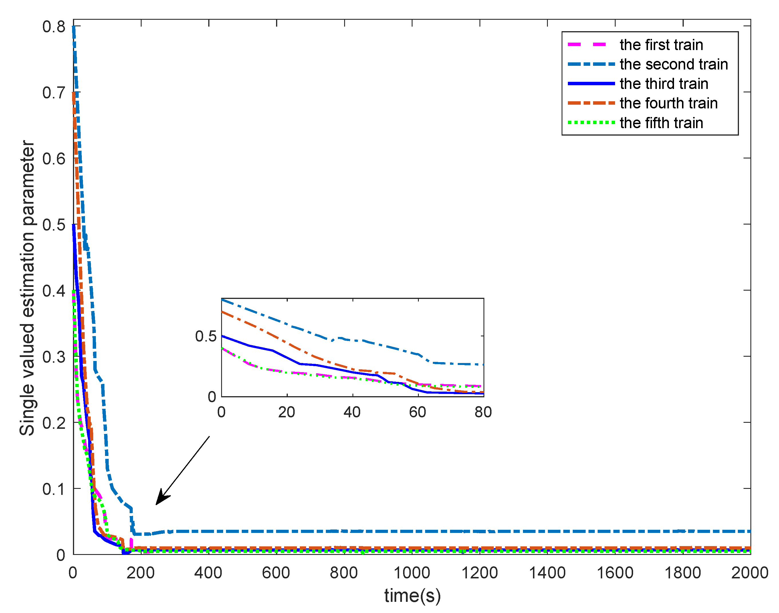
For the multiple trains single-value learning adaptive cooperative control with POC, the initial parameter values were set as ${\widehat{\Theta }}_1(0)=0.4$, ${\widehat{\Theta }}_2(0)=0.8$, ${\widehat{\Theta }}_3(0)=0.5$, ${\widehat{\Theta }}_4(0)=0.7$, ${\widehat{\Theta }}_5(0)=0.4$. The control parameters are fine-tuned using a trial-and-error scheme, and they were chosen as ${\alpha }_1={\alpha }_2={\alpha }_5=1$, ${\alpha }_3=0.4$, ${\alpha }_4=0.85$, ${\theta }_i=0.001$, ${\sigma }_{i,4}=0.3$.

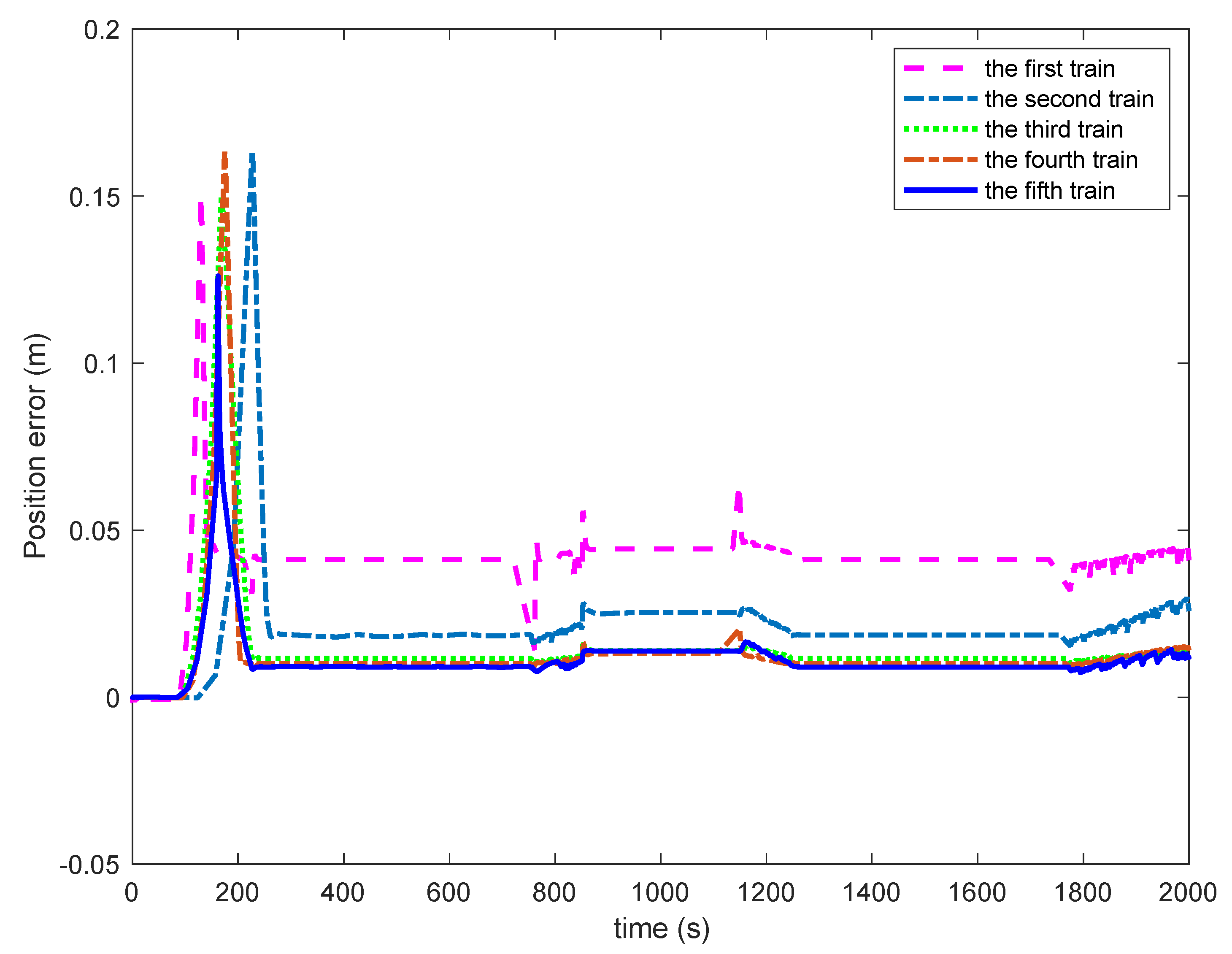
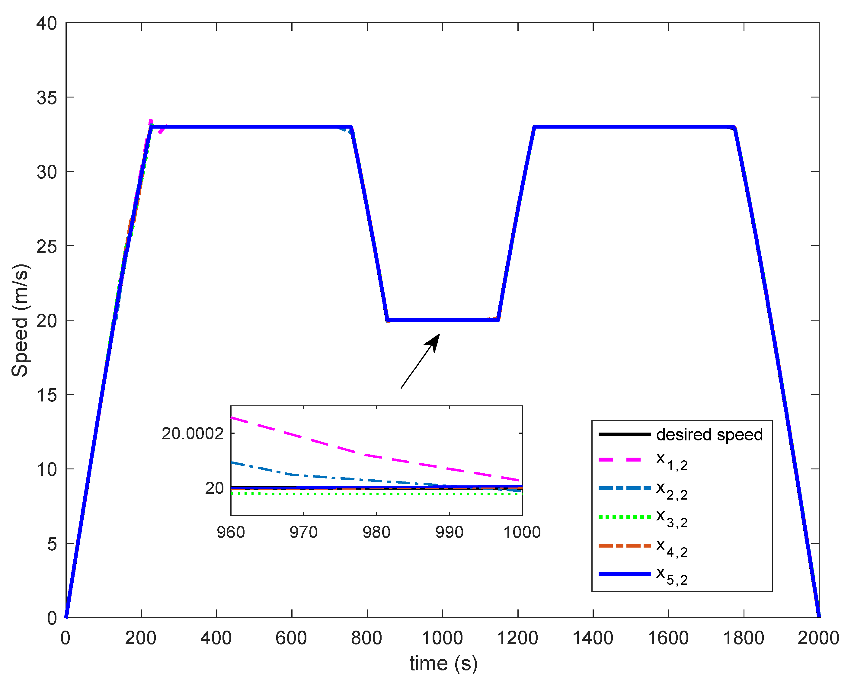
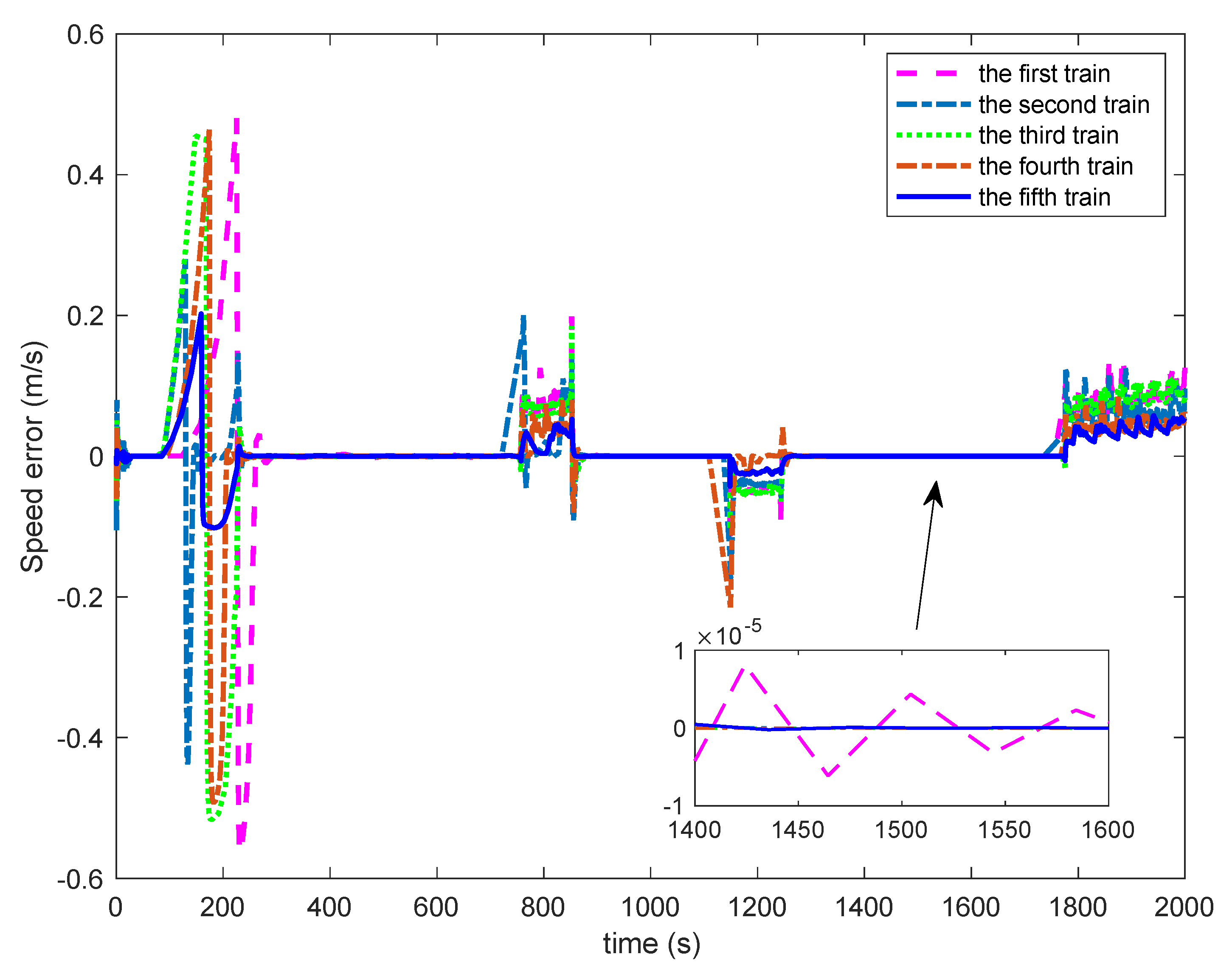
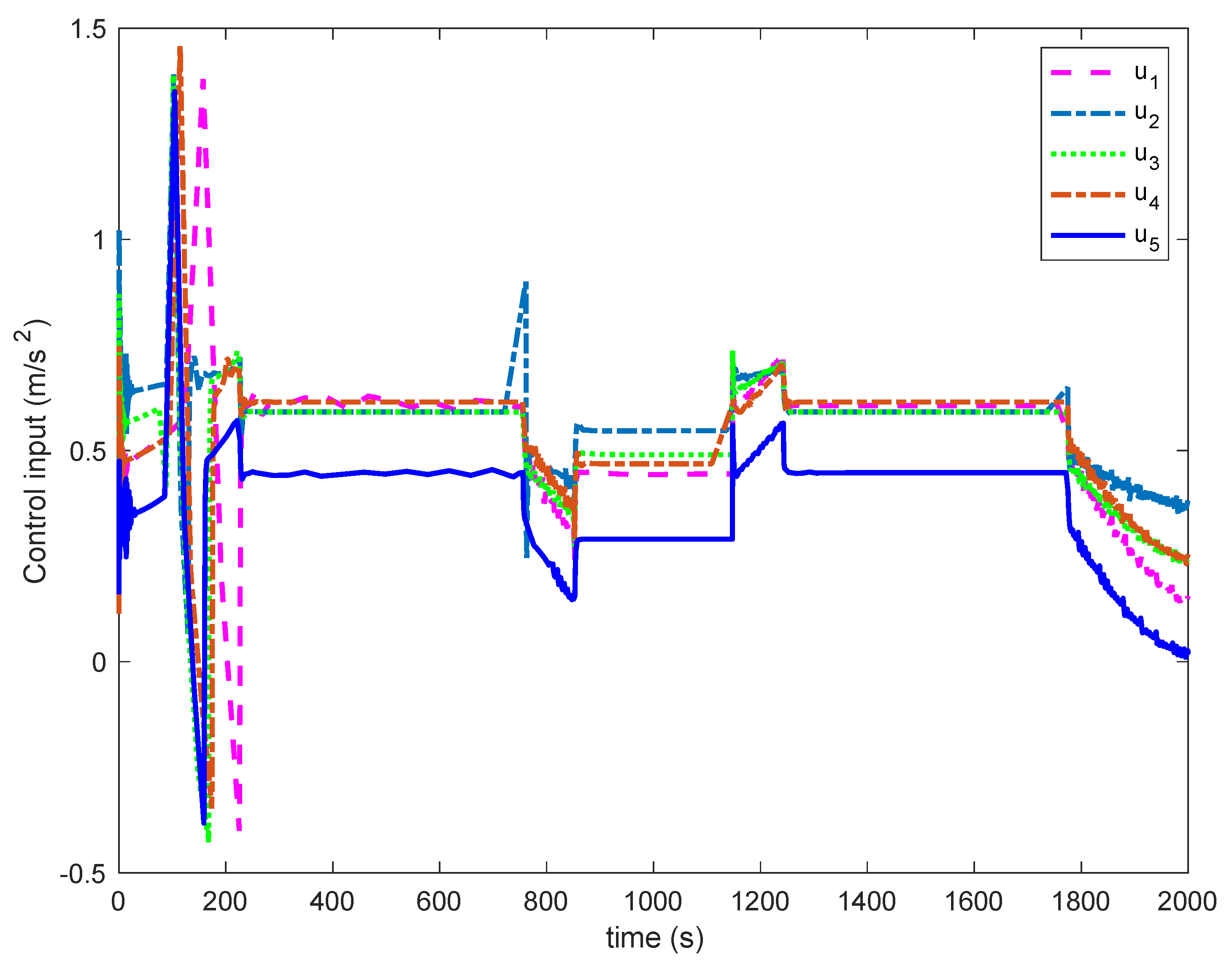
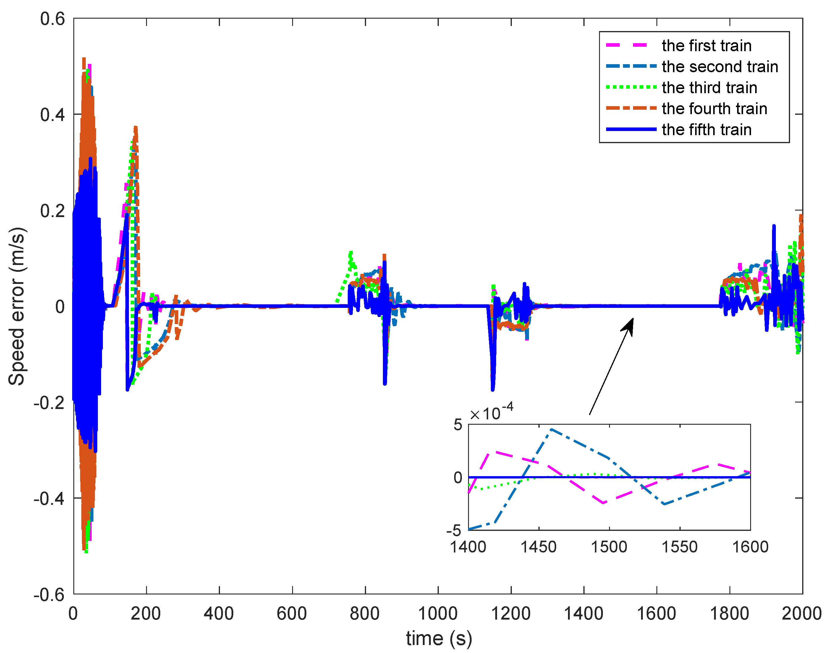
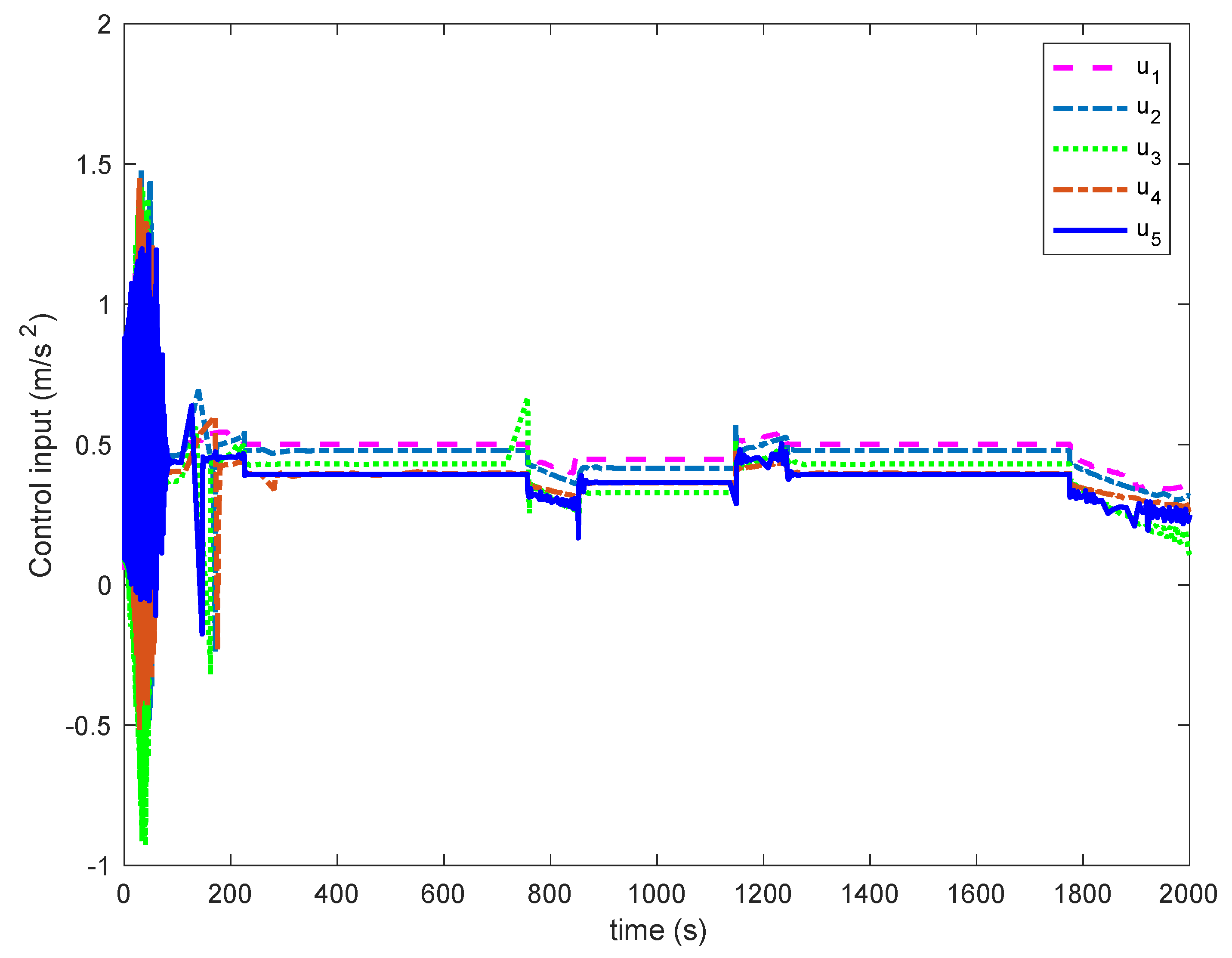
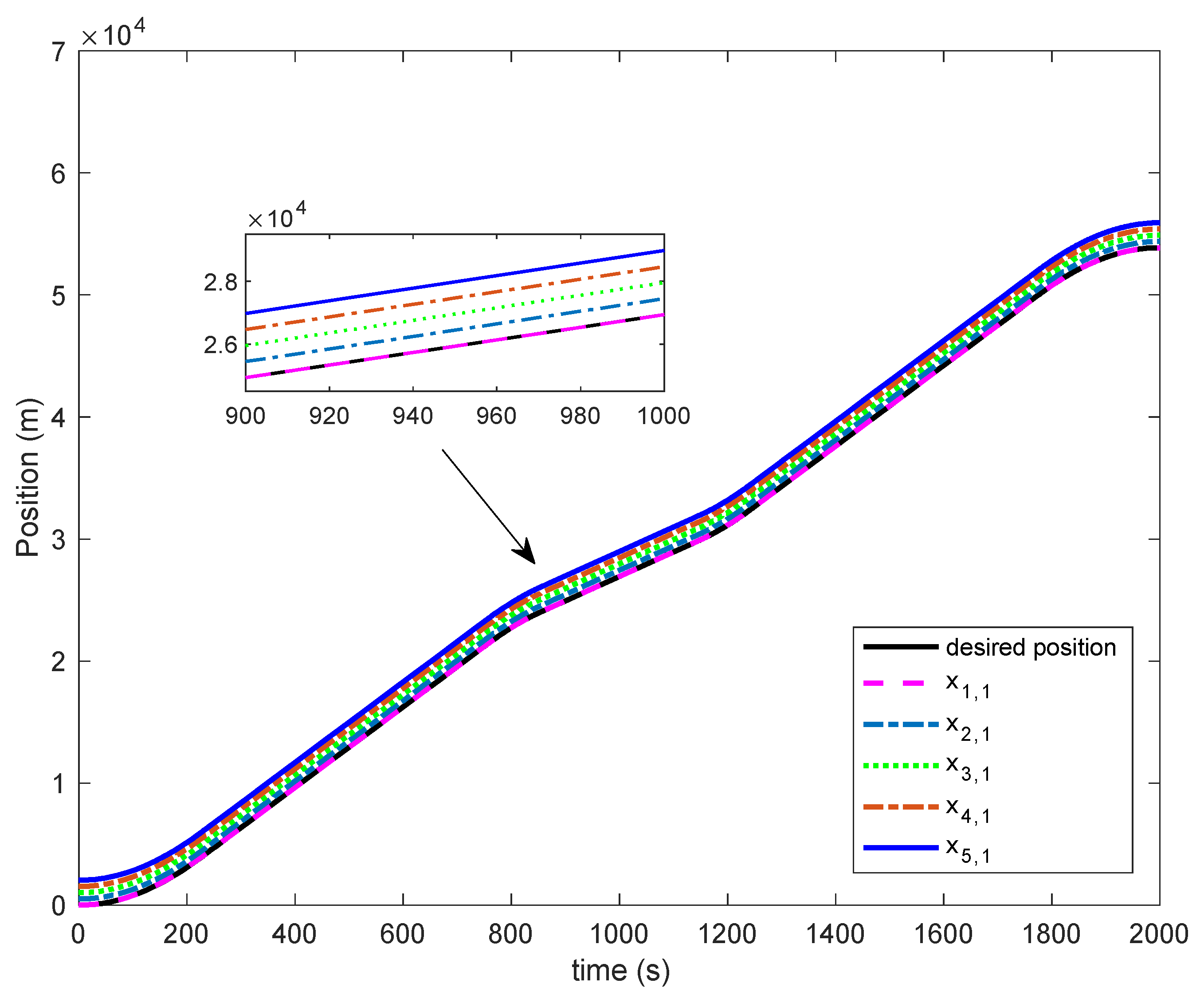
The simulation results of the multiple trains adaptive cooperative control with POC are shown in Figure 2, Figure 3, Figure 4, Figure 5 and Figure 6. Figure 2 and Figure 3 show the position tracking and position separation distance error curve of each train in the MTCC system respectively. Figure 4 and Figure 5 show the speed tracking and its error curve of each train in the MTCC system, respectively. Figure 6 shows the corresponding control input curve.

As can be seen from Figure 2, the first train achieves accurate tracking of the desired position outline. In the meantime, the following trains also have the fine tracking performance, and guarantee that the following trains maintain the set safe separation distance between two neighboring trains, which means the position tracking performance of the MTCC controller is excellent.

As can be seen from Figure 3, the separation distance error of each train matches the allowable range of stopping accuracy less than 0.2 m. The slight separation distance errors of two neighboring trains ensures the stability of the multiple trains operation and realizes the useful multiple trains cooperative control. It can also be observed that the position separation distance error of multiple trains does not “backward” propagate, i.e., the position error ${\tilde{x}}_{5,1}<{\tilde{x}}_{4,1}<{\tilde{x}}_{3,1}<{\tilde{x}}_{2,1}<{\tilde{x}}_{1,1}$, while the position error converges to a small size and the system performance is good.

From Figure 4 and Figure 5, it can be seen that the developed control algorithm can show true high-accuracy speed tracking, and the speed of each train is close to the desired speed, which effectively guarantees the safety of multiple trains cooperative operation. In particular, the speed control accuracy of multiple trains cooperative operation in cruise mode has obvious advantages.

The multiple trains control input curves of the proposed control algorithm, i.e., the acceleration curves of the multiple train’s operation, is given in Figure 6. The control input curve is relatively smoother overall, and when the train was running at 52 s to 248 s, the controller quickly switches the control input to keep the control accuracy in order to overcome the concentrated disturbances such as large external gradients and complex curves. The magnitude of this control input change can match the performance of train traction and braking. Therefore, the developed control algorithm has great position and speed tracking results and achieves the design objective of the distributed control laws for the cooperative operation of multiple trains.

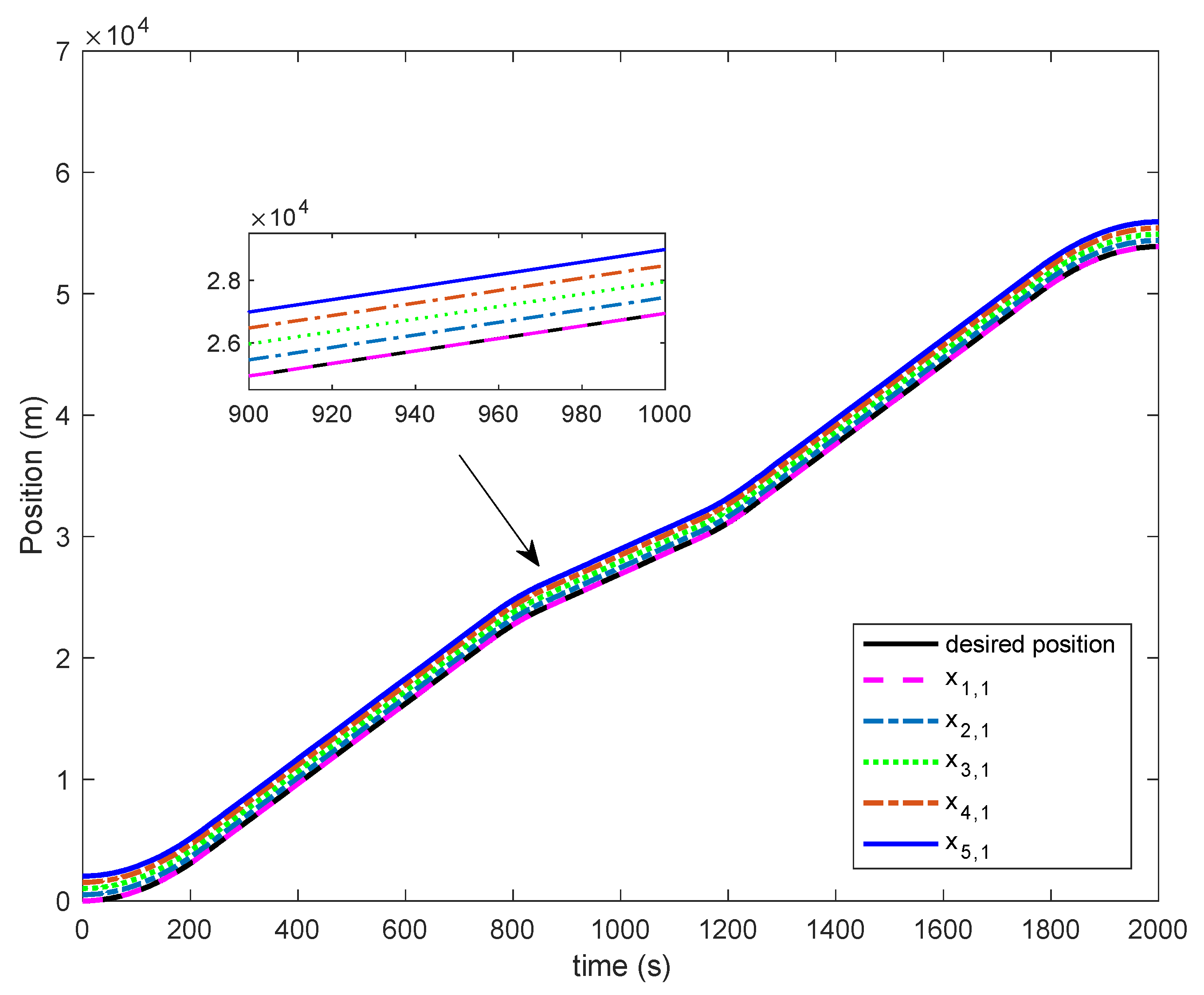
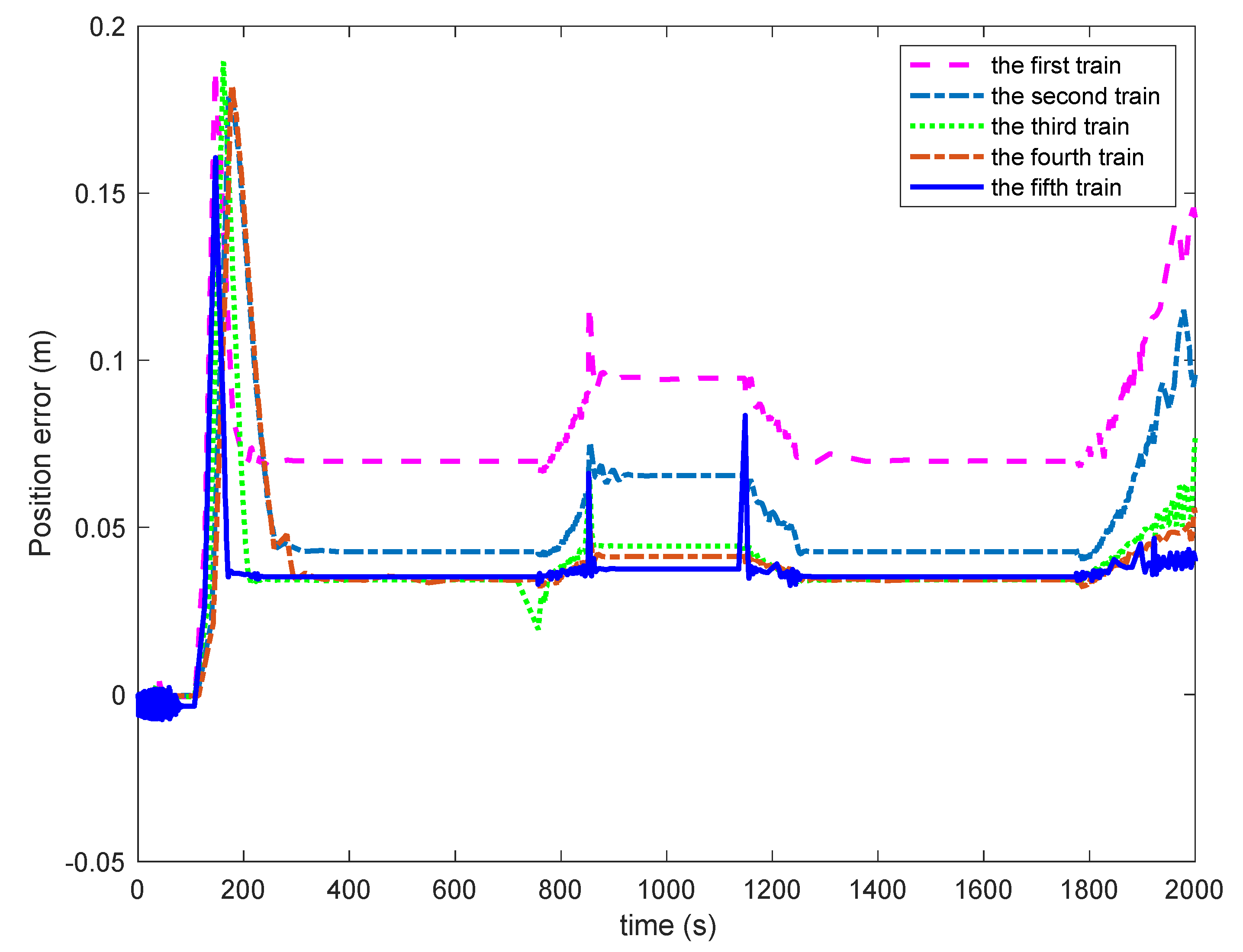
The simulation results of the multiple trains single-value learning adaptive cooperative control with POC are shown in Figure 7, Figure 8, Figure 9, Figure 10, Figure 11 and Figure 12. By applying the adaptive cooperative control in Equation (20) of single-value learning to each train in a multiple trains cooperative system with position output constrains, the evolution of the adaptive parameters is shown in Figure 7. It can be seen from Figure 7 that all the adaptive parameters converge to constants, which indicates the effectiveness of the designed single-value learning adaptive control algorithm in identifying these unknown parameters. The position tracking and the error curves of each train in the MTCC are given in Figure 8 and Figure 9, respectively. From the curves in the figure, it can be seen that the first train can follow the tracks of the desired train position curve with high precision, the following train can keep preinstall safety separation distance with the neighboring trains with minor error, and the tracking error of each train is within the tolerance range, which guarantees the safety of multiple trains cooperative operation and realizes the MTCC.

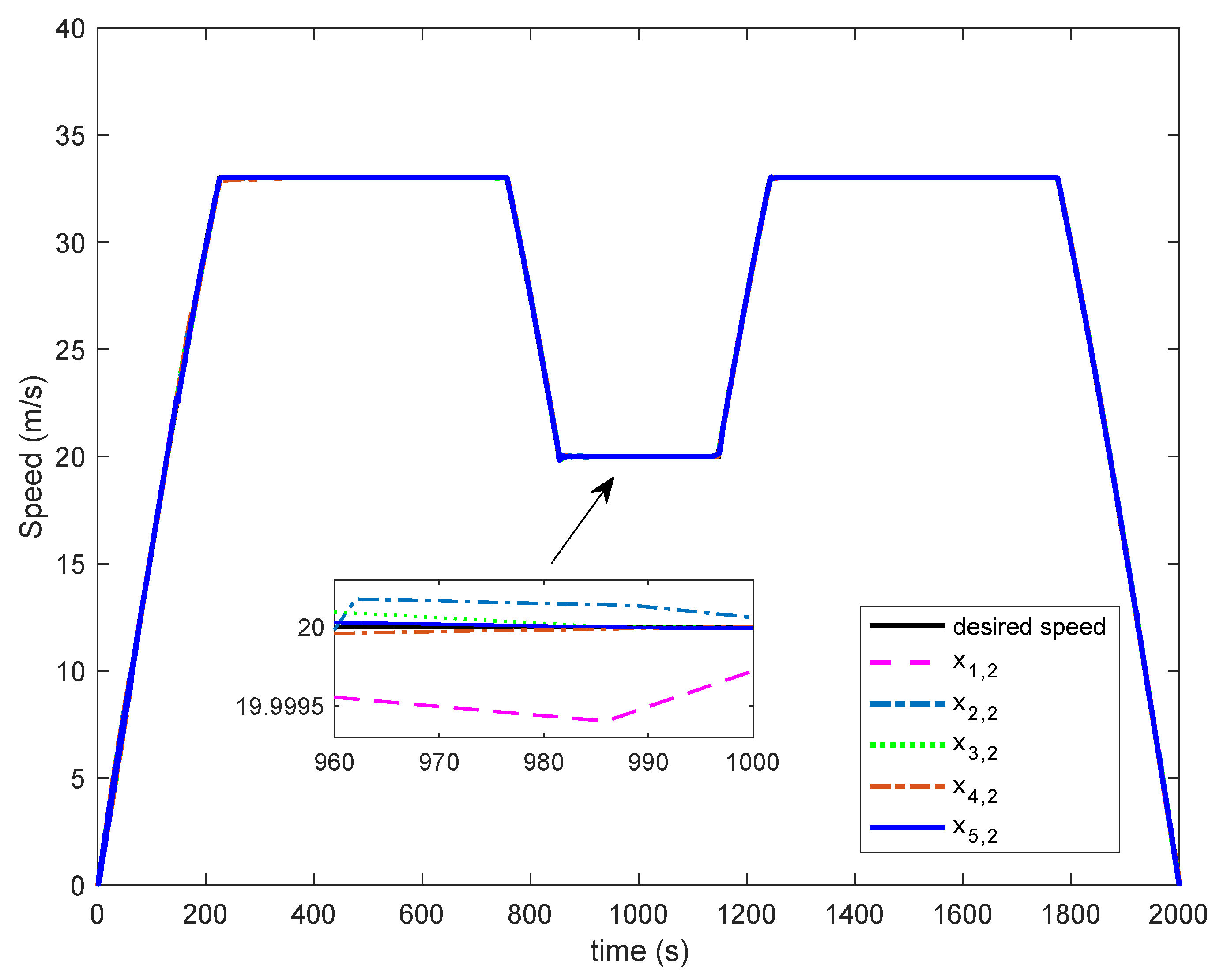
The speed and speed tracking error curves of each train are given in Figure 10 and Figure 11, respectively. From Figure 10 and Figure 11, it can be seen that the speed tracking effect is great and each train can automatically regulate the control input conferring to the data of the neighboring trains, as shown in Figure 12. In the section with sudden change of desired speed and complex route in Figure 10, that is, the train runs in 52 s to 248 s, the speed tracking error of each train in the multiple train cooperative operation system shown in Figure 11 fluctuates, but the speed error of the preceding trains does not affect the speed control of the tracking trains. The speed tracking error of each train decreases with the propagation of train number, that is, the fluctuation of speed tracking error of the fifth train is the smallest, which ensures the stability of multiple trains cooperative operation. In other acceleration and deceleration sections, the speed error of each train is significantly reduced. In particular, in the cruise section, the speed error of each train is almost zero, which has good control accuracy. As can be seen from Figure 12, when the trains are just started, the controller applies a large control input to overcome the external resistance. When the train runs normally, the control input remains stable. When the train continues to run for 52 s to 248 s, the controller adjusts the control input in order to maintain the control accuracy. The control inputs of other sections are relatively stable, even in acceleration and deceleration sections. The fluctuation is very small to meet the comfort of passengers. Thus, it can be seen that in the multiple trains single-value learning adaptive cooperative control system with POC, the trains can regulate their own operation status conferring to the operation data of the neighboring trains, which usefully ensures the safety of multiple trains cooperative operation, reduces the complexity of the controller, and provides a reference for the development and application of the new generation of MTCC system.

In addition, in order to demonstrate the performance and engineering practicality advantages of the controller proposed in this paper, the PID control algorithm is extensively applied to train operation control systems (such as the Beijing Metro Yizhuang Line) as selected in this paper, and the PID controller structure is chosen in the form of reference [27], with the PID controller parameters set as $K_{p,1}=0.05$, $K_{i,1}=0.01$, $K_{d,1}=0.03$, $K_{p,2}=0.15$, $K_{i,2}=0.03$, $K_{d,2}=0.013$, $K_{p,3}=0.13$, $K_{i,3}=0.035$, $K_{d,3}=0.014$, $K_{p,4}=0.11$, $K_{i,4}=0.032$, $K_{d,4}=0.012$, $K_{p,5}=0.1$, $K_{i,5}=0.03$, $K_{d,5}=0.02$.

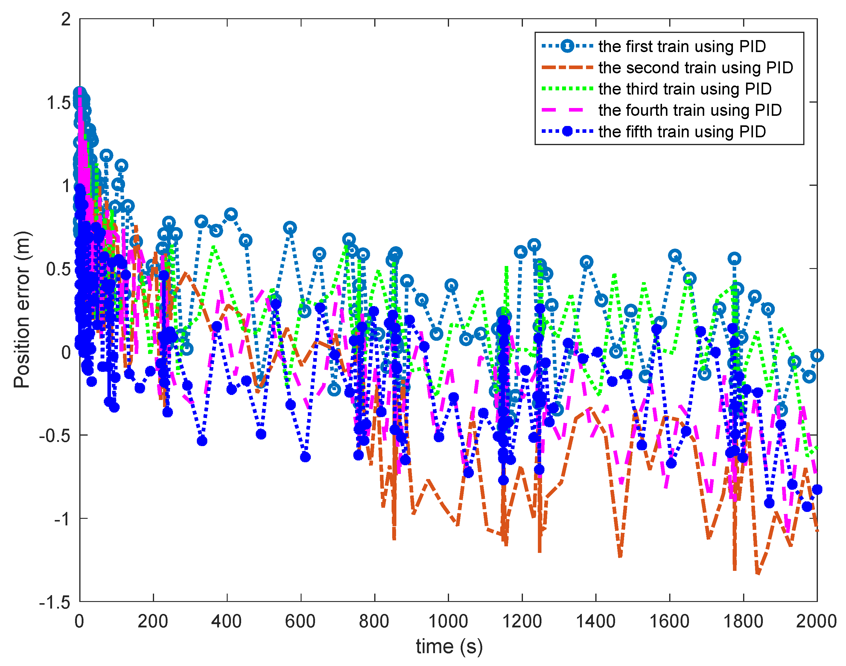
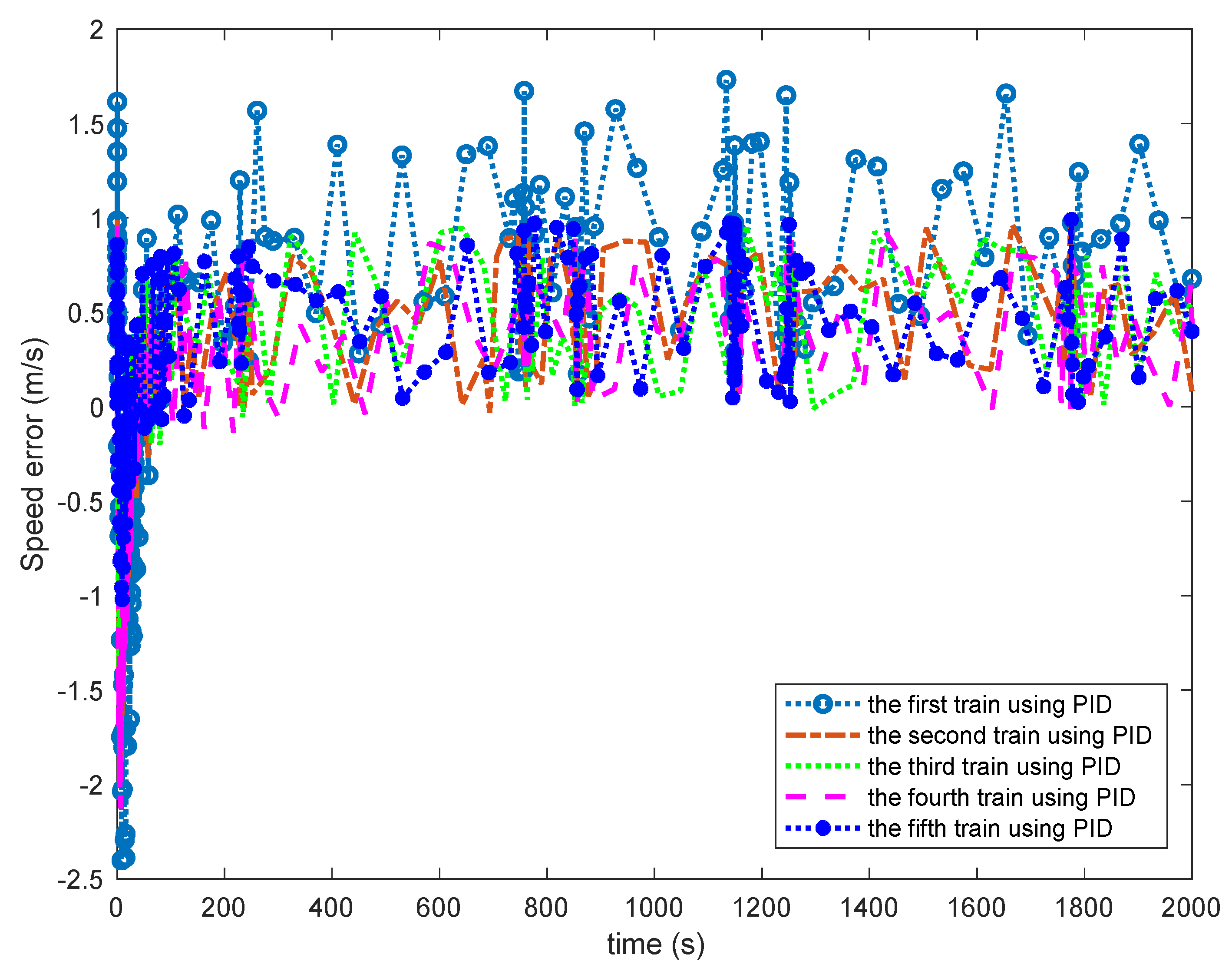
Figure 13 and Figure 14 give the position tracking errors and speed tracking errors under the PID controller. It can be seen from Figure 13 that the position tracking error of PID controller is distributed in the range of [−1.41, 1.58], which is relatively large as a whole. Due to the lack of adaptive mechanism of PID controller, the ability to deal with the change of train running resistance and external environment was not strong, and the degree of position tracking error decreasing in turn with the propagation of train number was not obvious. The overall position error is much larger than 0.2 m proposed in this paper, and there is continuous fluctuation. It can be seen from Figure 14 that the speed error of the PID controller varies widely, among which the speed error of the first train is the largest, and the speed error of the fifth train is improved, but there were overall fluctuations. Thus, the ability of PID controller to adjust its own operation state according to the operation information of adjacent trains is poor, and it is lack of adaptive ability to train operation resistance and external environment changes, so it is difficult to ensure the stability of multiple trains cooperative operation. By contrast, the multiple trains cooperative control method designed in this paper has great control performance and self-adaptability, and effectively ensures the safety of multiple trains cooperative operation.

5. Conclusions

In this paper, the cooperative operation control schemes for a class of nonlinear urban rail transit train systems are studied, and two position output-constrained adaptive control methods based on multi-agent collaboration are proposed. A set of orderly running urban rail trains are considered as a multi-agent system. The position output constrained adaptive learning controller uses the data of the train itself as well as the neighboring trains to enable the position and speed of each train to track the desired position and speed trajectory of the train. Among them, the train position errors of the two MTCC algorithms with POC meet the stopping accuracy of less than 0.2 m, respectively, and the position tracking error of their tracking trains is not affected by the position error of the preceding trains and gradually approaches 0, which ensures the stability of the multiple trains tracking operation. The introduction of the potential function ensures that the separation distance between any two neighboring trains is always kept within the designed safety range, which can be flexibly adjusted according to the conditions of train braking distance, safety redundancy distance, train length, and operation interval. The two position output constrained adaptive control methods based on multi-agent cooperation proposed in this paper can not only ensure the tracking operation safety of multiple urban rail trains, but also flexibly adjust the train operation interval and effectively improve the operation efficiency of urban rail system. In particular, single-value learning adaptive cooperative control method with POC for the multiple trains requires only one online parameter adjustment, which guarantees the engineering practicality of the algorithm while ensuring the lowest structural complexity of the MTCC algorithm which will promote the practicability of the theoretical work related to urban rail cooperative control. Additionally, the designed method is also suitable for irregular event interference in a certain range.

Although this paper has conducted in-depth research on the cooperative control problem and the model uncertainties problem for multiple urban rail trains, and achieved phased results, the cooperative control problem for the adjustment of urban rail trains’ operation status still needs further study due to the complexity of the cooperative adjustment process of urban rail trains and the time-varying characteristics of the train operation environment. Combined with practical engineering, future research will focus on the following areas:

• Multiple trains adaptive cooperative anti-disturbance control with position output constraints under model uncertainty constraints and longer lasting external multi-source disturbance. The dynamic behavior of multiple trains is related to many factors, excluding their own traction and braking force, but also by air resistance, tunnel resistance, ramp resistance, route condition changes, and the running state of the preceding trains and other random interference factors. So, it is very difficult to establish an accurate model that can portray so many factors, and at the same time, the model established by considering too many factors is too complicated. Therefore, while ensuring the simplicity of the control algorithm, the design considering the model uncertainties and longer lasting disturbance is the key to further improving the engineering practicability.
• Research on active fault-tolerant control of the running state adjustment process of urban rail multiple trains. The drift of train sensor parameters, the delay of multiple trains information interaction data transmission, and packet loss are unavoidable. Active fault-tolerant control that takes into account train sensor accuracy and communication channel capacity limitations will help to improve the reliability and applicability of multiple trains cooperative control.
• Research on more scenarios of multiple trains cooperative operation. In this paper, only the typical operation scenarios in multiple trains cooperative operation are considered, and other modes of actual train operation are not analyzed. Further exploration of multiple trains cooperative operation in other operation scenarios is needed to ensure the engineering practicality of the designed algorithm, which will promote the practicality of related theoretical work.

References

1. Yin, J.; Tang, T.; Yang, L.; Xun, J.; Huang, Y.; Gao, Z. Research and development of automatic train operation for railway transportation systems: A survey. Transp. Res. Part C Emerg. Technol. 2017, 85, 548–572. [Google Scholar] [CrossRef]
2. Dong, H.-R.; Gao, S.-G.; Ning, B.; Li, L. Extended fuzzy logic controller for high speed train. Neural Comput. Appl. 2013, 22, 321–328. [Google Scholar] [CrossRef]
3. Tan, L.T.; Huang, Y.N.; Li, L.Y. Driving curve algorithm for heavy haul train based on improved BP Neural Network. Railw. Comput. Appl. 2016, 25, 1–5. [Google Scholar]
4. Shi, W.S. Research on automatic train operation based on model-free adaptive control. J. China Railw. Soc. 2016, 38, 72–77. [Google Scholar]
5. Cao, Y.; Ma, L.; Zhang, Y. Application of fuzzy predictive control technology in automatic train operation. Clust. Comput. 2018, 22, 14135–14144. [Google Scholar] [CrossRef]
6. He, Z.Y.; Xu, N. Automatic train operation algorithm based on adaptive iterative learning control theory. J. Transp. Syst. Eng. Inf. Technol. 2020, 20, 69–75. [Google Scholar]
7. Yang, Y.F.; Cui, K.; Lv, X.J. Combined sliding model and PID control of automatic train operation system. J. China Railw. Soc. 2014, 36, 61–67. [Google Scholar]
8. Wang, Q.Y.; Wu, P. Precise automatic train stop control of algorithm based on adaptive terminal sliding mode control. J. China Railw. Soc. 2016, 38, 56–63. [Google Scholar]
9. Yin, J.; Chen, D.; Li, Y. Smart train operation algorithms based on expert knowledge and ensemble CART for the electric locomotive. Knowl. Based Syst. 2016, 92, 78–91. [Google Scholar] [CrossRef]
10. Ghasemi, A.; Kazemi, R.; Azadi, S. Stability analysis of bidirectional adaptive cruise control with asymmetric information flow. ARCHIVE Proc. Inst. Mech. Eng. Part C J. Mech. Eng. Sci. 2015, 229, 216–226. [Google Scholar] [CrossRef]
11. Albrecht, A.R.; Howlett, P.G.; Pudney, P.J.; Vu, X. Energy-efficient train control: From local convexity to global optimization and uniqueness. Automatica 2013, 49, 3072–3078. [Google Scholar] [CrossRef]
12. Li, S.K.; Li, X. Robust sampled-data cruise control scheduling of high speed train. Transp. Res. Part C Emerg. Technol. 2014, 46, 274–283. [Google Scholar] [CrossRef]
13. Ciccarelli, F.; Iannuzzi, D.; Tricoli, P. Control of metro-trains equipped with onboard super capacitors for energy saving and reduction of power peak demand. Transp. Res. Part C Emerg. Technol. 2012, 24, 36–49. [Google Scholar] [CrossRef]
14. Li, S.; Yang, L.; Gao, Z. Coordinated cruise control for high-speed train movements based on a multi-agent model. Transp. Res. Part C Emerg. Technol. 2015, 56, 281–292. [Google Scholar] [CrossRef]
15. Li, S.; Yang, L.; Gao, Z. Adaptive coordinated control of multiple high-speed trains with input saturation. Nonlinear Dyn. 2016, 83, 2157–2169. [Google Scholar] [CrossRef]
16. Gao, S.; Dong, H.; Ning, B.; Zhang, Q. Cooperative Prescribed Performance Tracking Control for Multiple High-Speed Trains in Moving Block Signaling System. IEEE Trans. Intell. Transp. Syst. 2018, 20, 2740–2749. [Google Scholar] [CrossRef]
17. Li, S.; Yang, L.; Gao, Z. Distributed optimal control for multiple high-speed train movement: An alternating direction method of multipliers. Automatica 2020, 112, 108646. [Google Scholar] [CrossRef]
18. Ji, H.; Hou, Z.; Zhang, R. Adaptive Iterative Learning Control for High-Speed Trains with Unknown Speed Delays and Input Saturations. IEEE Trans. Autom. Sci. Eng. 2015, 13, 260–273. [Google Scholar] [CrossRef]
19. Li, M.; Lin, P. Distributed Consensus of second-order multiagent systems with nonconvex input constraints. Int. J. Robust Nonlinear Control 2018, 11, 3657–3664. [Google Scholar]
20. Xiang, P.; Wang, X.; Mo, L. Cooperative H∞ Control of Multiple High-Speed Trains with Saturation Constraints. IEEE Access 2019, 7, 129437–129442. [Google Scholar] [CrossRef]
21. Lin, P.; Ren, W.; Gao, H. Distributed Velocity-Constrained Consensus of Discrete-Time Multi-Agent Systems with Nonconvex Constraints, Switching Topologies, and Delays. IEEE Trans. Autom. Control 2017, 62, 5788–5794. [Google Scholar] [CrossRef]
22. Lin, P.; Ren, W.; Yang, C.; Gui, W. Distributed Consensus of Second-Order Multiagent Systems with Nonconvex Velocity and Control Input Constraints. IEEE Trans. Autom. Control 2018, 63, 1171–1176. [Google Scholar] [CrossRef]
23. Tee, K.P.; Ge, S.S.; Tay, E.H. Barrier Lyapunov Functions for the control of output-constrained nonlinear systems. Automatica 2009, 45, 918–927. [Google Scholar] [CrossRef]
24. Ren, B.; Ge, S.S.; Tee, K.P.; Lee, T.H. Adaptive Neural Control for Output Feedback Nonlinear Systems Using a Barrier Lyapunov Function. IEEE Trans. Neural Netw. 2010, 21, 1339–1345. [Google Scholar] [CrossRef]
25. Chen, C.L.P.; Liu, Y.-J.; Wen, G.-X. Fuzzy Neural Network-Based Adaptive Control for a Class of Uncertain Nonlinear Stochastic Systems. IEEE Trans. Cybern. 2014, 44, 583–593. [Google Scholar] [CrossRef]
26. Yang, J.; Zhang, Y.; Jin, Y. Fully Automatic Operation Algorithm of Urban Rail Train Based on RBFNN Position Output Constrained Robust Adaptive Control. Algorithms 2021, 14, 264. [Google Scholar] [CrossRef]
27. Li, Z.X. Some issues on iterative learning control based high speed train operation control. Beijing Jiaotong Univ. 2016, 6, 89–93. [Google Scholar]
Figure 1. The diagram of multiple urban rail trains motion.
Algorithms 15 00138 g001
Figure 2. Desired position and position tracking performance of each train.
Algorithms 15 00138 g002
Figure 3. Position tracking error of each train.
Algorithms 15 00138 g003
Figure 4. Desired speed and speed tracking performance of each train.
Algorithms 15 00138 g004
Figure 5. Speed tracking error of each train.
Algorithms 15 00138 g005
Figure 6. Control input of each train.
Algorithms 15 00138 g006
Figure 7. Estimated parameter curves for single-value learning.
Algorithms 15 00138 g007
Figure 8. Desired position and position tracking curves for single-value learning.
Algorithms 15 00138 g008
Figure 9. Position tracking error curves for single-value learning.
Algorithms 15 00138 g009
Figure 10. Desired speed and speed tracking curves for single-valued learning.
Algorithms 15 00138 g010
Figure 11. Speed tracking error curves for single-value learning.
Algorithms 15 00138 g011
Figure 12. Control input curves for single-value learning.
Algorithms 15 00138 g012
Figure 13. Position tracking error curves of PID controller.
Algorithms 15 00138 g013
Figure 14. Speed tracking error curves of PID controller.
Algorithms 15 00138 g014
Publisher’s Note: MDPI stays neutral with regard to jurisdictional claims in published maps and institutional affiliations.