Guided Semi-Supervised Non-Negative Matrix Factorization

Abstract

Classification and topic modeling are popular techniques in machine learning that extract information from large-scale datasets. By incorporating a priori information such as labels or important features, methods have been developed to perform classification and topic modeling tasks; however, most methods that can perform both do not allow for guidance of the topics or features. In this paper, we propose a novel method, namely Guided Semi-Supervised Non-negative Matrix Factorization (GSSNMF), that performs both classification and topic modeling by incorporating supervision from both pre-assigned document class labels and user-designed seed words. We test the performance of this method on legal documents provided by the California Innocence Project and the 20 Newsgroups dataset. Our results show that the proposed method improves both classification accuracy and topic coherence in comparison to past methods such as Semi-Supervised Non-negative Matrix Factorization (SSNMF), Guided Non-negative Matrix Factorization (Guided NMF), and Topic Supervised NMF.

1. Introduction

Understanding latent trends within large-scale, complex datasets is a key component of modern data science pipelines, leading to downstream tasks such as classification and clustering. In the setting of textual data contained within a collection of documents, non-negative matrix factorization (NMF) has proven itself as an effective, unsupervised tool for this exact task [1,2,3,4,5,6,7], with trends represented by topics. Whilst such fully unsupervised techniques bring great flexibility in application, it has been demonstrated that learned topics may not have the desired effectiveness in downstream tasks [8]. In particular, certain related features may be strongly weighted in the data, yielding highly related topics that do not capture the variety of trends effectively [9]. To counteract this effect, some level of supervision may be introduced to steer learnt topics towards being more meaningful and representative, and thus improve the quality of downstream analyses. Semi-Supervised NMF (SSNMF) [10,11,12,13,14] utilizes class label information to simultaneously learn a dimensionality-reduction model and a model for a downstream task such as classification. Guided NMF [15] instead incorporates user-designed seed words to “guide” topics towards capturing a more diverse range of features, leveraging (potentially little) supervision information to drive the learning of more balanced, distinct topics. Topic Supervised NMF (TS-NMF) [16] associates label information to latent topics to achieve better modeling results. Despite a distinction between the supervision information and goals of Guided NMF, SSNMF, and TS-NMF, there are certainly mutual relationships: knowledge of class labels can be leveraged to improve the quality of learnt topics (in terms of scope, mutual exclusiveness, and self-coherence), whilst a priori seed words for each class can improve classification.

With these heuristics in mind, the contributions of this paper are as follows. We first analyze the characteristics of both classical and state-of-the-art NMF variants for classification and topic modeling tasks. We then propose the Guided Semi-Supervised NMF (GSSNMF), a model that incorporates both seed word information and class labels in order to simultaneously learn topics and perform classification. Our experimental results demonstrate that utilizing both forms of supervision information concurrently offers improvements to both the topic modeling and classification tasks, while producing highly interpretable results.

2. Related Work

2.1. Classical Non-Negative Matrix Factorization

Non-negative matrix factorization (NMF) is a powerful framework for performing unsupervised tasks such as topic modeling and clustering [1]. Given a target dimension $k<min\{d,n\}$, the classical NMF method approximates a non-negative data matrix $\mathit{X}\in {\mathbb{R}}^{d\times n}$ by the product of two non-negative low-rank matrices: the dictionary matrix $\mathit{W}=[{\mathbf{w}}_1,{\mathbf{w}}_2,\cdots ,{\mathbf{w}}_k]\in {\mathbb{R}}_{\ge 0}^{d\times k}$ and the coding matrix $\mathit{H}=[{\mathbf{h}}_1,{\mathbf{h}}_2,\cdots ,{\mathbf{h}}_n]\in {\mathbb{R}}_{\ge 0}^{k\times n}$. Both matrices $\mathit{W}$ and $\mathit{H}$ can be found by solving the optimization problem

$$\underset{\mathit{W}\in {\mathbb{R}}_{\ge 0}^{d\times k},\mathit{H}\in {\mathbb{R}}_{\ge 0}^{k\times n}}{argmin}\frac{1}{2}{\parallel \mathit{X}-\mathit{W}\mathit{H}\parallel }_F^2,$$

(1)

where ${\parallel \mathit{A}\parallel }_F^2={\sum }_{i,j}{a}_{ij}^2$ is the Frobenius norm of $\mathit{A}$, and the constant of $\frac{1}{2}$ is to ease the calculation when taking the gradient. In the context of topic modeling, the dimension k is the number of desired topics. Each column of $\mathit{W}$ encodes the strength of every dictionary word’s association with a learned topic, and each column of $\mathit{H}$ encodes the relevance of every topic for a given document in the corpus. By enforcing non-negativity constraints, NMF methods can learn topics and document classes with high interpretability [1,7].

2.2. Semi-Supervised NMF

Besides topic modeling, one variant of classical NMF, Semi-Supervised NMF (SSNMF) [10,11,14] is designed to further perform classification. SSNMF introduces a masking matrix $\mathit{L}=[{\ell }_1,\cdots ,{\ell }_n]\in {\mathbb{R}}_{\ge 0}^{p\times n}$ and a label matrix $\mathit{Z}=[{\mathbf{z}}_1,\cdots ,{\mathbf{z}}_n]\in {\mathbb{R}}_{\ge 0}^{p\times n}$, where p is the number of classes and n is the number of documents. The masking matrix $\mathit{L}$ is defined as:

$${\ell }_j=\left\{\begin{array}{cc}{\mathbf{1}}_p,\hfill & \mathrm{if}\mathrm{the}\mathrm{label}\mathrm{of}\mathrm{document}{x}_j\mathrm{is}\mathrm{known}\hfill \\ {\mathbf{0}}_p,\hfill & \mathrm{otherwise},\hfill \end{array}\right.$$

(2)

where ${\mathbf{1}}_p={[1,\cdots ,1]}^T\in {\mathbb{R}}^p$ and ${\mathbf{0}}_p={[0,\cdots ,0]}^T\in {\mathbb{R}}^p$. Note that the masking matrix $\mathit{L}$ splits the label information into train and test sets. Each column ${\mathbf{z}}_i$ is a binary encoding vector such that, if the document ${\mathit{x}}_i$ belongs to class j, the $j^{th}$ entry of ${\mathbf{z}}_i$ is 1, and otherwise it is set to be 0. The dictionary matrix $\mathit{W}$, coding matrix $\mathit{H}$, and label dictionary matrix $\mathit{C}$ can be found by solving the optimization problem

$$\underset{\mathit{W}\in {\mathbb{R}}_{\ge 0}^{d\times k},\mathit{H}\in {\mathbb{R}}_{\ge 0}^{k\times n},\mathit{C}\in {\mathbb{R}}_{\ge 0}^{p\times k}}{argmin}\underset{\mathrm{classical}\mathrm{NMF}}{\underbrace{\frac{1}{2}{\parallel \mathit{X}-\mathit{W}\mathit{H}\parallel }_F^2}}+\underset{\mathrm{label}\mathrm{information}}{\underbrace{\frac{\mu }{2}{\parallel \mathit{L}\odot (\mathit{Z}-\mathit{C}\mathit{H})\parallel }_F^2}},$$

(3)

where $\mu >0$ is a regularization parameter and $\mathit{A}\odot \mathit{B}$ denotes entry-wise multiplication between matrix $\mathit{A}$ and $\mathit{B}$. Matrices $\mathit{W}$ and $\mathit{H}$ can be interpreted in the same way as classical NMF. Matrix $\mathit{C}$ can be viewed as the dictionary matrix for the label matrix $\mathit{Z}$.

2.3. Guided NMF

Due to the fully unsupervised nature of classical NMF, the generated topics may suffer from redundancy or lack of cohesion when the given data set is biased towards a set of featured words [8,9,15]. Guided NMF [15] addresses this by guiding the topic outputs through incorporating flexible user-specified seed word supervision. Each word in a given list of s seed words can be represented as a sparse binary seed vector $\mathbf{v}\in {\mathbb{R}}^d$, whose entries are zero except for some positive weights at entries corresponding to the seed word feature. The corresponding binary seed matrix $\mathit{Y}\in {\mathbb{R}}_{\ge 0}^{d\times s}$ can be constructed as

$$\mathit{Y}=[{\mathbf{v}}_{\mathbf{1}},\cdots ,{\mathbf{v}}_{\mathbf{s}}]\in {\mathbb{R}}_{\ge 0}^{d\times s}.$$

For a given data matrix $\mathit{X}$ and a seed matrix $\mathit{Y}$, Guided NMF seeks a dictionary matrix $\mathit{W}$, coding matrix $\mathit{H}$, and topic supervision matrix $\mathit{B}$ by considering the optimization problem

$$\underset{\mathit{W}\in {\mathbb{R}}_{\ge 0}^{d\times k},\mathit{H}\in {\mathbb{R}}_{\ge 0}^{k\times n},\mathit{B}\in {\mathbb{R}}_{\ge 0}^{k\times s}}{argmin}\underset{\mathrm{classical}\mathrm{NMF}}{\underbrace{\frac{1}{2}{\parallel \mathit{X}-\mathit{W}\mathit{H}\parallel }_F^2}}+\underset{\mathrm{guiding}}{\underbrace{\frac{\lambda }{2}{\parallel \mathit{Y}-\mathit{W}\mathit{B}\parallel }_F^2}},$$

(4)

where $\lambda >0$ is a regularization parameter. Matrices $\mathit{W}$ and $\mathit{H}$ can be interpreted in the same way as classical NMF. Matrix $\mathit{B}$ can help identify topics that form from the influence of seed words.

2.4. Topic Supervised NMF

Given the binary label matrix $\mathit{Z}$, also known as the supervision matrix, Topic Supervised NMF (TS-NMF) [16] is able to supervise the classical NMF method to potentially improve topic modeling results. For a given data matrix $\mathit{X}$ and a supervision matrix $\mathit{Z}$, TS-NMF finds the dictionary matrix $\mathit{W}$ and coding matrix $\mathit{H}$ by solving the optimization problem:

$$\underset{\mathit{W}\in {\mathbb{R}}_{\ge 0}^{d\times k},\mathit{H}\in {\mathbb{R}}_{\ge 0}^{k\times n}}{argmin}\frac{1}{2}{\parallel \mathit{X}-(\mathit{W}\odot \mathit{Z})\mathit{H}\parallel }_F^2,$$

(5)

where the matrices $\mathit{W}$ and $\mathit{H}$ can be interpreted in the same way as in classical NMF. The supervision matrix $\mathit{Z}$ constrains the importance weights of ${\mathit{W}}_{ij}$ by enforcing ${\mathit{W}}_{ij}$ to be 0 whenever ${\mathit{Z}}_{ij}$ is 0. By doing so, TS-NMF is able to prescribe a subspace of the latent topic space for labeled documents for improved topic modeling results. Note that the number of latent topics must equal the number of different labels.

3. Proposed Method

Recall that SSNMF is able to classify different documents through given label information, while Guided NMF can guide the content of generated topics via a priori seed words. We propose a more general model, Guided Semi-Supervised NMF (GSSNMF) that can leverage both label information and important seed words to improve performance in both multi-label classification and topic modeling. Heuristically, we see that, for classification, the user-specified seed words aid SSNMF in distinguishing between each class label and thus improve classification accuracy. For topic modeling, the known label information enables Guided NMF to better cluster similar documents, improving topic coherence and interpretability. Our algorithm combines these and seeks to approximately solve the optimization problem

$$\underset{\mathit{W}\in {\mathbb{R}}_{\ge 0}^{d\times k},\mathit{H}\in {\mathbb{R}}_{\ge 0}^{k\times n},\mathit{B}\in {\mathbb{R}}_{\ge 0}^{k\times s},\mathit{C}\in {\mathbb{R}}_{\ge 0}^{p\times k}}{argmin}\underset{\mathrm{classical}\mathrm{NMF}}{\underbrace{\frac{1}{2}{\parallel \mathit{X}-\mathit{W}\mathit{H}\parallel }_F^2}}+\underset{\mathrm{guiding}}{\underbrace{\frac{\lambda }{2}{\parallel \mathit{Y}-\mathit{W}\mathit{B}\parallel }_F^2}}+\underset{\mathrm{label}\mathrm{information}}{\underbrace{\frac{\mu }{2}{\parallel \mathit{L}\odot (\mathit{Z}-\mathit{C}\mathit{H})\parallel }_F^2}},$$

(6)

where matrices $\mathit{W}$, $\mathit{H}$, $\mathit{Y}$, $\mathit{B}$, $\mathit{L}$, $\mathit{Z}$, and $\mathit{C}$ and constants $\lambda$ and $\mu$ can be interpreted in the same way as in SSNMF and Guided NMF. Note that, if we simply set either $\lambda$ or $\mu$ to be 0, GSSNMF reduces to SSNMF or Guided NMF, respectively.

To solve (6), we propose an algorithm that utilizes a multiplicative update scheme akin to those in [11,17]. In a manner similar to gradient descent, at each step, each of the four matrices $\mathit{W},\mathit{H},\mathit{B},\mathit{C}$ are updated in turn, while viewing the other three as fixed. The derivation of these updates is provided in Appendix A, and the updating process is presented in Algorithm 1. Note that, as with other multiplicative update methods for NMF variants, the loss is monotone [2].

Algorithm 1: GSSNMF with multiplicative updates.

    We will demonstrate the strength of GSSNMF by considering different combinations of the parameters $\lambda$ and $\mu$, and comparing the implementations of this method with Classical NMF, SSNMF, Guided NMF, and TS-NMF through real-life applications in the following section.

4. Experiments

In this section, we evaluate the performances of our GSSNMF on the California Innocence Project dataset [18] and the 20 Newsgroups dataset [19]. Specifically, we compare GSSNMF with SSNMF for performance in classification (measured by the Macro-F1 score, i.e., the averaged F1-score which is sensitive to different distributions of different classes [20]) and with classical NMF, TS-NMF, and Guided NMF for performance in topic modeling (measured by the $\mathcal{C}$ coherence score [21]).

4.1. Pre-Processing of the CIP Dataset

A nonprofit, clinical law school program hosted by the California Western School of Law, the California Innocence Project (CIP) focuses on freeing wrongfully-convicted prisoners, reforming the criminal justice system, and training upcoming law students [18]. Every year, the CIP receives over 2000+ requests for help, each containing a case file of legal documents. Within each case file, the Appellant’s Opening Brief (AOB) is a legal document written by an appellant to argue for innocence by explaining the mistakes made by the court. This document contains crucial information about the crime types relevant to the case, as well as potential evidence within the case [18]. For our final dataset, we include all AOBs in case files that have assigned crime labels, totaling 203 AOBs. Each AOB is thus associated with one or more of thirteen crime labels: assault, drug, gang, gun, kidnapping, murder, robbery, sexual, vandalism, manslaughter, theft, burglary, and stalking.

To pre-process data, we remove numbers, symbols, and stopwords according to the NLTK English stopwords list [22] from all AOBs; we also perform stemming to reduce inflected words to their original word stem. Following the work of [18,23,24], we apply term-frequency inverse document frequency (TF-IDF) [25] to our dataset of AOBs. TF-IDF retains the relative simplicity of a bag-of-words representation while additionally moderating the impact of words that are common to every document, which can be detrimental to performance [26,27,28,29]. We generated the corpus matrix $\mathit{X}$ with parameters max_df = 0.8, min_df=0.04, and max_features = 700 in the function TfidfVectorizer.

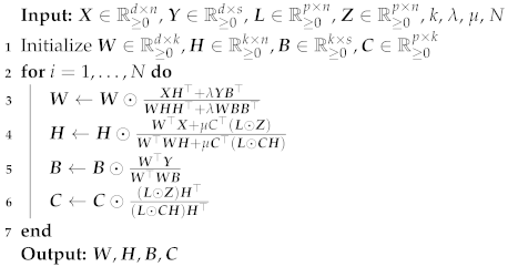
For our topic modeling methods, we need to preset the potential number of topics, which corresponds to the rank of corpus matrix $\mathit{X}$. To determine the proper range of the number of topics, we analyze the singular values of $\mathit{X}$. The magnitudes of singular values are positively related to the increment in proportion variance explained by adding on more topics, or increasing rank, to split the corpus matrix $\mathit{X}$ [30]. In this way, we use the number of singular values to approximate the rank of $\mathit{X}$. 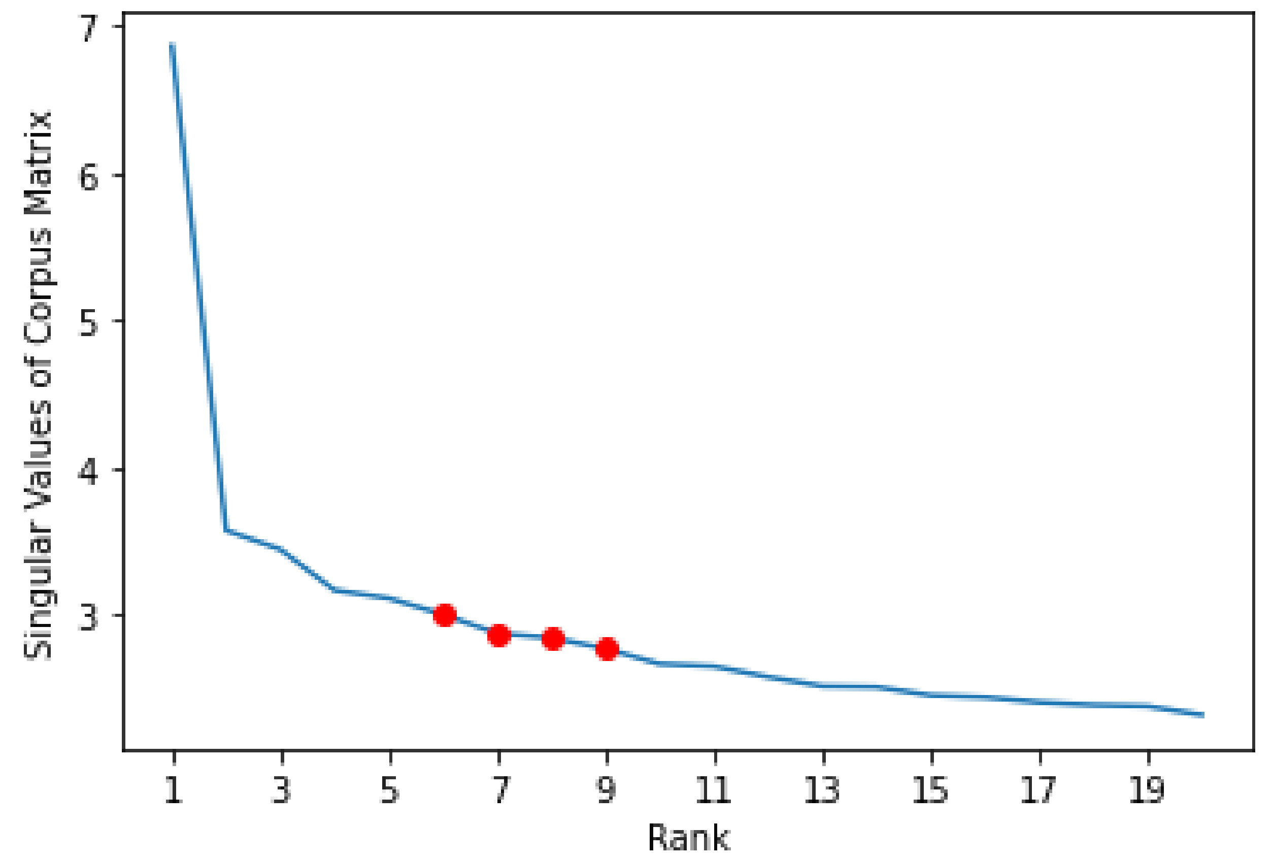Figure 1 plots the magnitudes of the singular values of corpus matrix $\mathit{X}$ against the number of singular values, which is also the approximated rank. By examining this plot, we see that a range for potential rank is between 6 to 9, since the magnitudes of the singular values start to level off around this range.

4.2. Classification on the CIP Dataset

Taking advantage of Cross-Validation methods [31], we randomly split all AOBs into $70\%$ training set with labeled information and $30\%$ testing set without labels. In practice, $70\%$ of the columns of the masking matrix $\mathit{L}$ are set to ${\mathbf{1}}_p$ for the training set, and the rest are set to ${\mathbf{0}}_p$ for the testing set. As a result, the label matrix $\mathit{Z}$ is masked by $\mathit{L}$ into a corresponding training label matrix ${\mathit{Z}}_{\mathrm{train}}$ and a corresponding testing label matrix ${\mathit{Z}}_{\mathrm{test}}$. We then perform SSNMF and GSSNMF to reconstruct ${\mathit{Z}}_{\mathrm{test}}$ by setting the number of topics as 8. Given the multi-label characteristics of the AOBs, we compare the performance between SSNMF and GSSNMF with a measure of classification accuracy: the Macro F1-score, which is designed to access the quality of multi-label classification on ${\mathit{Z}}_{\mathrm{test}}$ [20]. The Macro F1-score is defined as

$$\mathrm{Macro}\mathrm{F}1-\mathrm{score}=\frac{1}{p}\sum _{i=1}^p\mathrm{F}1-{\mathrm{score}}_i,$$

(7)

where p is the number of labels and F1-score${}_i$ is the F1-score for topic i. Notice that the Macro F1-score treats each class with equal importance; thus, it will penalize models which only perform well on major labels but not minor labels. In order to handle the multi-label characteristics of the AOB dataset, we first extract the number of labels assigned to each AOB in the testing dataset. Then, for each corresponding column i of the reconstructed ${\mathit{Z}}_{\mathrm{test}}$, we set the largest $j_i$ elements in each column to be 1 and the rest to be 0, where $j_i$ is the actual number of labels assigned to the ith document in the testing set.

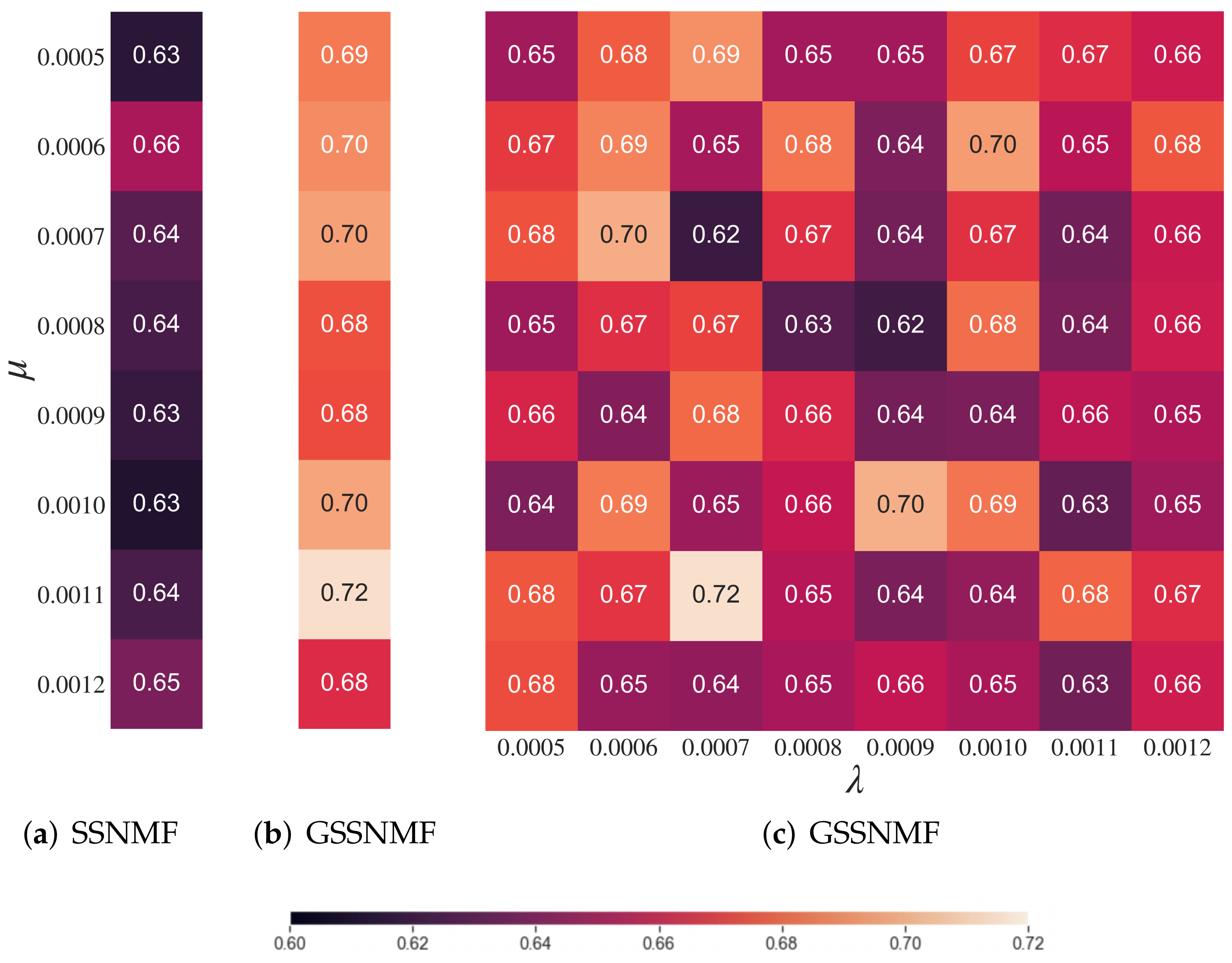
We first tune the parameter of $\mu$ in SSNMF to identify a proper range of $\mu$ for which SSNMF performs the best on the AOB dataset under the Macro F1-score. Then, for each selected $\mu$ in the proper range, we run GSSNMF with another range of $\lambda$. While there are various choices of seed words, we naturally pick the class labels themselves as seed words for our implementation of GSSNMF. As a result, for each combination of $\mu ,\lambda \in \{0.0005,0.0006,\cdots ,0.0012\}$, we conduct 10 independent Cross-Validation trials and average the Macro F1-scores. The results are displayed in Figure 2.

We see that, in general, when incorporating the extra information from seed words, GSSNMF has a higher Macro F1-score than SSNMF. As an example, we extract the reconstructed testing label matrix by SSNMF and GSSNMF along with the actual testing label matrix from a single trial. In this instance, SSNMF has a Macro F1-score of 0.672 while GSSNMF has a Macro F1-score of 0.765. By comparing the reconstructed matrices with the actual label matrix, we generate two difference matrices representing the correct and incorrect labels produced by the two methods respectively. The matrices are visualized in Figure 3. Given the fact that murder is a major label, without the extra information from seed words, SSNMF makes many incorrect classifications on the major label murder. In comparison, through user-specified seed words, GSSNMF not only reduces the number of incorrect classifications along the major label murder, but also better evaluates the assignment of other labels, achieving an improved classification accuracy.

4.3. Topic Modeling on the CIP Dataset

In this section, we test the performance of GSSNMF for topic modeling by comparing it with Classical NMF, Guided NMF, and TS-NMF on the CIP AOB dataset. Specifically, we conduct experiments for the range of rank identified in Section 4.1, running tests for various values of $\lambda$ and $\mu$ for each rank. To measure the effectiveness of the topics discovered by Guided NMF and GSSNMF, we calculate the topic coherence score defined in [21] for each topic. The coherence score ${\mathcal{C}}_i$ for each topic i with N most probable keywords is given by

$${\mathcal{C}}_i=\sum _{b=2}^N\sum _{\ell =1}^{b-1}log\frac{P(w_b^{\left(i\right)},w_{\ell }^{\left(i\right)})+1}{P\left(w_{\ell }^{\left(i\right)}\right)}.$$

(8)

In the above Equation (8), $P\left(w\right)$ denotes the document frequency of keyword w, which is calculated by counting the number of documents that keyword w appears in at least once. $P(w,w^{\prime })$ denotes the co-document frequency of keyword w and $w^{\prime }$, which is obtained by counting the number of documents that contain both w and $w^{\prime }$. In general, the topic coherence score seeks to measure how well the keywords that define a topic make sense as a whole to a human expert, providing a means for consistent interpretation of accuracy in topic generation. A large positive $\mathcal{C}$ coherence score indicates that the keywords from a topic are highly cohesive, as judged by a human expert.

Since we are judging the performance of methods that generate multiple topics, we calculate coherence scores $\mathcal{C}$ for each topic that is generated by Guided NMF or GSSNMF and then take the average. Thus, our final measure of performance for each method is the averaged coherence score ${\mathcal{C}}_{\mathrm{avg}}$:

$${\mathcal{C}}_{avg}=\frac{{\sum }_{i=1}^k{C}_i}{k},$$

(9)

where k is the number of topics (or rank) we have specified.

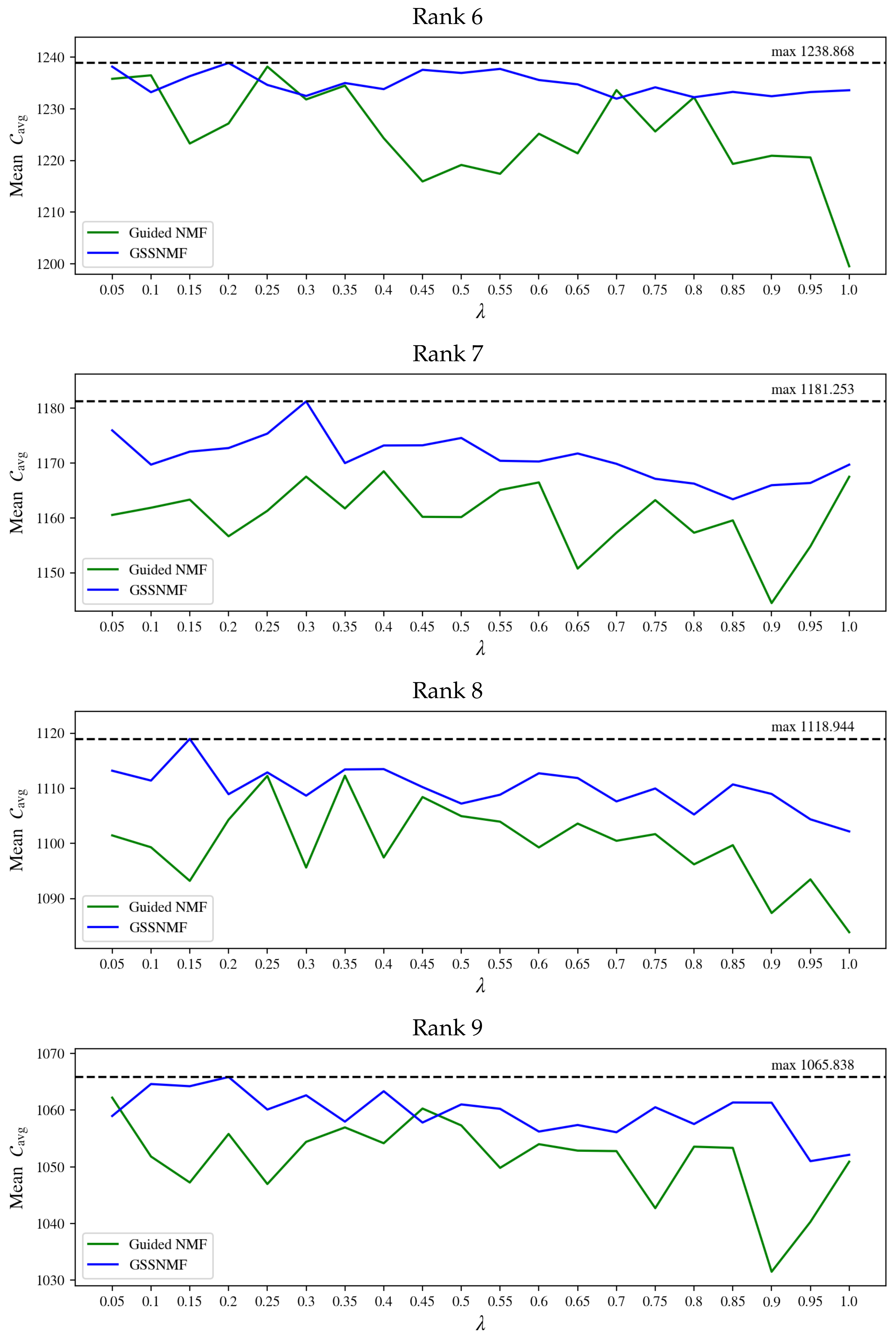
As suggested by Figure 1, a proper rank falls between 6 and 9. Starting with the generation of 6 topics from the AOB dataset, we first find a range of $\lambda$ in which Guided NMF generates the highest mean ${\mathcal{C}}_{\mathrm{avg}}$ over 10 independent trials. In our computations, we use the top 30 keywords of each topic to generate each coherence score; then, for each trial, we obtain an individual ${\mathcal{C}}_{\mathrm{avg}}$, allowing us to average the 10 ${\mathcal{C}}_{\mathrm{avg}}$ from the 10 trials into the mean ${\mathcal{C}}_{\mathrm{avg}}$. Based on the proper range of $\lambda$, we then choose a range of $\mu$ for our GSSNMF to incorporate the label information into topic generation. Again, for each pair of $(\lambda ,\mu )$, we run 10 independent trials of GSSNMF and calculate ${\mathcal{C}}_{\mathrm{avg}}$ for each trial to generate a mean ${\mathcal{C}}_{\mathrm{avg}}$. With these ranges in mind, we work towards the following goal: for a given “best" $\lambda$ of Guided NMF, we improve topic generation performance by implementing GSSNMF with a “best” $\mu$ that balances how much weight GSSNMF should place on the new information of predetermined labels for each document. We then repeat the same process for ranks 7, 8, and 9, and plot the mean ${\mathcal{C}}_{\mathrm{avg}}$ against each $\lambda$ in Figure 4. The corresponding choice of $\mu$ can be found in Appendix B. We can see that, most of the time, for a given $\lambda$, we are able to find such $\mu$ that GSSNMF can generate a higher mean ${\mathcal{C}}_{\mathrm{avg}}$ than Guided NMF in topic modeling across various ranks. Ultimately, we also see that a GSSNMF result always outperforms even the highest-performing Guided NMF result.

In

Table 1. Topic modeling results of guided NMF and GSSNMF for Rank 7.

Guided NMF Results ($\mathit{\lambda }=0.4$)
Topic 1	Topic 2	Topic 3	Topic 4	Topic 5	Topic 6	Topic 7
gang	burglari	murder	accomplic	gang	instruct	identif
member	sexual	shot	corrobor	member	murder	eyewit
crip	strike	hous	robberi	expert	manslaught	photo
activ	admiss	detect	instruct	beer	lesser	lineup
phone	instruct	vehicl	murder	estrada	theori	suggest
murder	threat	phone	codefend	hispan	degre	suspect
photo	object	apart	abet	tattoo	passion	photograph
territori	discret	robberi	commiss	intent	abet	pack
associ	impos	want	special	men	voluntari	procedur
shot	sex	firearm	conspiraci	robberi	premedit	expert
Coherence Score $\mathcal{C}$ per Topic:
1112.94	1388.307	1290.817	921.023	1109.453	1123.185	1090.895
Averaged Coherence Score ${\mathcal{C}}_{\mathrm{avg}}$: 1148.089
GSSNMF Results ($\lambda =0.3,\mu =0.006$)
Topic 1	Topic 2	Topic 3	Topic 4	Topic 5	Topic 6	Topic 7
murder	instruct	detect	identif	gang	gang	burglari
accomplic	manslaught	phone	eyewit	member	member	strike
corrobor	lesser	probat	photo	crip	expert	sexual
vehicl	murder	waiver	lineup	associ	beer	robberi
robberi	self	plea	suggest	expert	hispan	impos
shot	passion	interrog	suspect	activ	shot	discret
abet	theori	confess	photograph	intent	estrada	punish
intent	voluntari	interview	pack	premedit	men	sex
degre	heat	admiss	procedur	prove	tattoo	feloni
hous	spont	transcript	reliabl	firearm	male	threat
Coherence Score $\mathcal{C}$ per Topic:
1215.826	1024.617	1188.975	1184.333	1180.321	1084.33	1281.146
Averaged Coherence Score ${\mathcal{C}}_{\mathrm{avg}}$: 1165.65

, we provide an example of the outputs of topic modeling from Guided NMF using $\lambda =0.4$ and from GSSNMF using $\lambda =0.3$ and $\mu =0.006$ for a rank of 7. Note that we output only the top 10 keywords under each identified topic group for ease of viewing, but our coherence scores are measured using the top 30 keywords. Thus, while the top 10 probable keywords of the generated topics may look similar across the two methods, and the coherence scores calculated from the top 30 probable keywords reveal that GSSNMF produces more coherent topics as a whole in comparison to Guided NMF. Specifically, GSSNMF demonstrates an ability to produce topics with similar levels of coherence (as seen from the small variance in individual coherence scores $\mathcal{C}$ of each topic), while Guided NMF produces topics that may vary in level of coherence (as seen from the large variance in individual coherence scores $\mathcal{C}$ for each topic). This further illustrates that GSSNMF is able to use the additional label information to execute topic modeling with better coherence.

We also compare GSSNMF to two other NMF methods—classical NMF and TS-NMF—on the basis of topic modeling performance on the CIP dataset. Following our methodology for applying GSSNMF to this data, we ran 10 independent trials of classical NMF for each rank from 6 to 9 and computed the mean ${\mathcal{C}}_{\mathrm{avg}}$ for each rank. The results for classical NMF, Guided NMF, and GSS-NMF using ranks 6–9 are summarized in 

Table 2. Coherence of topics generated by Classical NMF, Guided NMF, and GSSNMF for CIP data.

	Rank	6	7	8	9
${\mathcal{C}}_{\mathrm{avg}}$	Classical NMF	1247.219	1181.154	1133.603	1070.618
	Guided NMF	1227.161	1167.535	1112.29	1058.728
	GSSNMF	1238.868	1181.253	1118.944	1065.837
Best GSSNMF Parameters		$\mu =0.016$	$\mu =0.006$	$\mu =0.014$	$\mu =0.01$
		$\lambda =0.2$	$\lambda =0.3$	$\lambda =0.15$	$\lambda =0.2$

. For the rank 6–9 approximations, while classical NMF slightly outperforms GSSNMF on the basis of the topic coherence score ${\mathcal{C}}_{\mathrm{avg}}$, GSSNMF retains the advantage that the generated topics are guided by a priori information, whereas classical NMF has no such guarantee. As noted in Section 2.4, when TS-NMF is applied for topic modeling, the number of latent topics must be exactly equal to the number of different labels. In the case of the CIP data, the AOBs have 13 possible labels, so we ran TS-NMF on the CIP data with a rank of 13, computing ${\mathcal{C}}_{\mathrm{avg}}$ over 10 independent trials. TS-NMF (using rank 13) had ${\mathcal{C}}_{\mathrm{avg}}=1458.732$, which outperforms our recorded GSSNMF results for the same data. This could be a result of the structure of the CIP dataset, together with being constrained to use a rank of 13 when applying TS-NMF. As shown in 

Table 3. Similar topics generated by TS-NMF.

Top 10 Words from Selected TS-NMF Topics
Topic 1	Topic 2	Topic 3	Topic 4
gang	gang	gang	accomplic
member	estrada	member	gang
instruct	expert	circumstanti	robberi
expert	member	premedit	instruct
assault	tattoo	murder	corrobor
beer	identif	instruct	identif
object	opin	deliber	intent
intent	territori	accomplic	special
injuri	primari	intent	feloni
men	activ	shot	abet

, at least four of the topics generated by TS-NMF were all clearly related to gang activity, which is one of the labels used by TS-NMF. While the resulting topics are highly coherent, the abundance of closely related topics obscures the latent structure of the data. This arises from the fact that TS-NMF must use a rank exactly equal to the number of different labels, which may not accurately reflect the true low-rank structure of the data. In this case, we see that this splits larger topics into more specific subtopics that have several words in common. This increases ${\mathcal{C}}_{\mathrm{avg}}$, but the resulting topics do not correspond well to the original labels.

4.4. Pre-Processing of the 20 Newsgroups Dataset

The original 20 Newsgroups dataset [19] is a collection of around 20,000 individual news documents. The dataset is organized into 20 different Newsgroups, each corresponding to a topic. For this experiment, we select documents from nine newsgroups. From each group, we randomly select 200 documents. As a result, our dataset contains a total of 1800 documents from the categories: comp.graphics, comp.sys.mac.hardware, sci.crypt, rec.motorcycles, rec.sport.baseball, sci.med, sci.space, talk.politics.guns, talk.religion.misc. We then evaluate the performance of GSSNMF on this subset of the original 20 Newsgroups data.

To pre-processs the data, we follow the same approaches as for the CIP data, namely, removing numbers, symbols, and stopwords, and stemming the remaining words. Using TF-IDF, we generated the corpus matrix $\mathit{X}$ with parameters max_df = $0.8$, and max_features = 2000 in the function TfidfVectorizer.

To determine the potential number of topics for these data, we also analyze the singular values of $\mathit{X}$. Figure 5 demonstrates the distribution of the singular values of $\mathit{X}$, which is also the potential number of topics. From Figure 5, one can see that the potential topic number should be between 6 to 9 where the magnitudes of the singular values start to level off.

4.5. Classification on the 20 Newsgroups Dataset

For classification, we follow a similar approach to [14] so that comparisons may be drawn. Namely, we group the nine selected topics into five classes, as described in

Table 4. Classes, topics, and seed words for 20 Newsgroups.

Class	Topics	Seed Words
Computers	comp.graphics, comp.sys.mac.hardware	graphics, hardware
Science	sci.crypt, sci.med, sci.space	cryptography, medical, space
Politics	talk.politics.guns	guns
Religion	talk.religion.misc	god
Recreation	rec.motorcycles, rec.sport.baseball	motorcycle, baseball

, i.e., we view the data as containing five classes, which may be subdivided into nine latent topics. Training label data are then constructed for these five classes, and seed words are designed for each of the nine topics. Further details in the methodology are identical to those in Section 4.2.

Similarly to the analysis of the CIP dataset, we begin by tuning $\mu$ to yield the best possible results for SSNMF, again in terms of the Macro F1-score. Scores for selected values of $\mu$ around this maximum are given in Figure 6. For these values of $\mu$, we then run GSSNMF over a range of $\lambda$, the best scores following this tuning are presented in Figure 6.

We see that, as in the CIP data experiments, GSSNMF is able to leverage the additional seed word information to outperform the classification performance of SSNMF. The smaller absolute difference in scores compared to the CIP results is likely due to the overall higher scores for this dataset.

4.6. Topic Modeling on the 20 Newsgroups Dataset. Note That TS-NMF’s Rank Has to Equal the Number of Classes; as a Result, It Only Has Rank 9 Topic Modeling Result

In this section, we test the performance of GSSNMF for topic modeling by comparing it with Classical NMF, Guided NMF, and TS-NMF on the 20 Newsgroups data. For each proper rank indicated by Figure 5, we run a range of $\mu$ and $\lambda$ to select the best parameter for Guided NMF and GSSNMF. Note that both classical NMF and TS-NMF do not require the selection of $\mu$ and $\lambda$. To quantify the performance, we also measure the averaged coherence score ${\mathcal{C}}_{\mathrm{avg}}$ as described in Equation (9) using the top 30 keywords of each topic. The resulting ${\mathcal{C}}_{\mathrm{avg}}$ scores are recorded in

Table 5. Coherence of topics generated by Classical NMF, Guided NMF, TS-NMF, and GSSNMF for 20 Newsgroups data.

Rank		6	7	8	9
${\mathcal{C}}_{\mathrm{avg}}$	Classical NMF	980.860	940.967	874.404	832.409
	Guided NMF	858.361	798.737	741.057	714.796
	TS-NMF	-	-	-	856.786
	GSSNMF	984.443	942.678	881.626	843.399
Best GSSNMF Parameters		$\mu =0.0085$ $\lambda =0.1$	$\mu =0.012$ $\lambda =0.3$	$\mu =0.012$ $\lambda =0.3$	$\mu =0.0001$ $\lambda =0.5$

along with the choices of parameters. The ${\mathcal{C}}_{\mathrm{avg}}$ scores indicate that our GSSNMF algorithm outperforms the other NMF methods in rank 6, 7, and 8 topic modeling. For the rank 9 topic modeling, even though TS-NMF outperforms our GSSNMF, the ${\mathcal{C}}_{\mathrm{avg}}$ scores are fairly close. In addition, GSSNMF does generate the highest overall ${\mathcal{C}}_{\mathrm{avg}}$ score in the rank 6 topic modeling. This is an indication that the “true rank" for topic modeling in this subset of 20 Newsgroups data might not be 9; however, TS-NMF does not offer such flexibility and freedom to choose different ranks for topic modeling other than fixing the rank to be the number of labels. This further illustrates that GSSNMF can use additional label information for a more coherent topic model while not being limited by the additional label information.

5. Conclusions and Future Works

In this paper, we analyze the characteristics of SSNMF (Section 2.2), Guided NMF (Section 2.3), and TS-NMF (Section 2.4) concerning the tasks of classification and topic modeling. From these methods, we propose a novel NMF model, namely the GSSNMF, which combines characteristics of SSNMF, Guided NMF, and TS-NMF. SSNMF utilizes label information for classification, Guided NMF leverages user-specific seed words to guided topic content, and TS-NMF uses selected label information to inform topic modeling. To carry out classification and topic modeling simultaneously, ourGSSNMF uses additional label information to improve the coherence of topic modeling results while incorporating seed words for more accurate classification. Taking advantage of multiplicative updates, we provide a solver for GSSNMF and then evaluate its performance on real-life data.

In general, GSSNMF is able to out-perform SSNMF on the task of classification. The extra information from the seed words contributes to a more accurate classification result. Specifically, SSNMF tends to focus on the most prevalent class label and classifies all documents into that class label. Unlike SSNMF, the additional information from choosing seed words as the class labels can help GSSNMF treat each class label equally and avoid the trivial solution of classifying every single document into the most prevalent class label. Additionally, GSSNMF is able to generate more coherent topics when compared to Guided NMF on the task of topic modeling. The extra information from the known label matrix can help GSSNMF better identify which documents belong to the same class. As a result, GSSNMF generates topics with higher and less variable coherence scores. When compared with TS-NMF, GSSNMF also reveals its flexibility in choosing the latent topic number, which potentially helps it to generate a set of more coherent topics and meanwhile a higher classification accuracy.

While there are other variants of SSNMF according to [14], we developed GSSNMF only based on the standard Frobenius norm. In the future, we plan to make use of other comparable measures like the information divergence, and derive a corresponding multiplicative updates solver. In addition, across all the experiments, we selected the parameters $\lambda$ and $\mu$, which put weight on the seed word matrix and label matrix, respectively, based on the experimental results. In our continued work, we plan to conduct error analysis to determine how each parameter affects the other parameter and the overall approximation results. Particularly, for a given parameter $\lambda$ or $\mu$, we hope to identify an underlying, hidden relationship that allows us to quickly pick a matching $\mu$ or $\lambda$, respectively, that maximizes GSSNMF performance.

References

1. Lee, D.D.; Seung, H.S. Learning the parts of objects by non-negative matrix factorization. Nature 1999, 401, 788–791. [Google Scholar] [CrossRef] [PubMed]
2. Seung, D.; Lee, L. Algorithms for non-negative matrix factorization. Adv. Neural Inf. Process. Syst. 2001, 13, 556–562. [Google Scholar]
3. Arora, S.; Ge, R.; Moitra, A. Learning topic models–going beyond SVD. In Proceedings of the 2012 IEEE 53rd Annual Symposium on Foundations of Computer Science, New Brunswick, NJ, USA, 20–23 October 2012; pp. 1–10. [Google Scholar]
4. Kuang, D.; Choo, J.; Park, H. Nonnegative Matrix Factorization for Interactive Topic Modeling and Document Clustering. In Partitional Clustering Algorithms; Springer: Berlin/Heidelberg, Germany, 2015; pp. 215–243. [Google Scholar]
5. Wu, W.; Kwong, S.; Hou, J.; Jia, Y.; Ip, H.H.S. Simultaneous dimensionality reduction and classification via dual embedding regularized nonnegative matrix factorization. IEEE Trans. Image Process. 2019, 28, 3836–3847. [Google Scholar] [CrossRef] [PubMed]
6. Wu, W.; Jia, Y.; Wang, S.; Wang, R.; Fan, H.; Kwong, S. Positive and negative label-driven nonnegative matrix factorization. IEEE Trans. Circuits Syst. Video Technol. 2020, 31, 2698–2710. [Google Scholar] [CrossRef]
7. Xu, W.; Liu, X.; Gong, Y. Document Clustering Based on Non-Negative Matrix Factorization. In Proceedings of the 26th Annual International ACM SIGIR Conference on Research and Development in Informaion Retrieval, Toronto, ON, Canada, 28 July–1 August 2003; pp. 267–273. [Google Scholar]
8. Chang, J.; Gerrish, S.; Wang, C.; Boyd-graber, J.; Blei, D. Reading Tea Leaves: How Humans Interpret Topic Models. In Proceedings of the Advances in Neural Information Processing Systems, Vancouver, BC, Canada, 7–10 December 2009. [Google Scholar]
9. Jagarlamudi, J.; Daumé III, H.; Udupa, R. Incorporating Lexical Priors into Topic Models. In Proceedings of the Proceedings of the 13th Conference of the European Chapter of the Association for Computational Linguistics, Avignon, France, 23–27 April 2012; Association for Computational Linguistics: Avignon, France, 2012; pp. 204–213. [Google Scholar]
10. Chen, Y.; Rege, M.; Dong, M.; Hua, J. Non-negative matrix factorization for semi-supervised data clustering. Knowl. Inf. Syst. 2008, 17, 355–379. [Google Scholar] [CrossRef]
11. Lee, H.; Yoo, J.; Choi, S. Semi-Supervised Nonnegative Matrix Factorization. IEEE Signal Process. Lett. 2010, 17, 4–7. [Google Scholar]
12. Jia, Y.; Kwong, S.; Hou, J.; Wu, W. Semi-supervised non-negative matrix factorization with dissimilarity and similarity regularization. IEEE Trans. Neural Netw. Learn. Syst. 2019, 31, 2510–2521. [Google Scholar] [CrossRef] [PubMed]
13. Jia, Y.; Liu, H.; Hou, J.; Kwong, S. Semisupervised adaptive symmetric non-negative matrix factorization. IEEE Trans. Cybern. 2020, 51, 2550–2562. [Google Scholar] [CrossRef] [PubMed]
14. Haddock, J.; Kassab, L.; Li, S.; Kryshchenko, A.; Grotheer, R.; Sizikova, E.; Wang, C.; Merkh, T.; Madushani, R.W.M.A.; Ahn, M. Semi-Supervised NMF Models for Topic Modeling in Learning Tasks. Available online: https://arxiv.org/pdf/2010.07956 (accessed on 29 January 2022).
15. Vendrow, J.; Haddock, J.; Rebrova, E.; Needell, D. On a Guided Nonnegative Matrix Factorization. In Proceedings of the ICASSP 2021—2021 IEEE International Conference on Acoustics, Speech and Signal Processing (ICASSP), Toronto, ON, Canada, 6–11 June 2021; pp. 3265–32369. [Google Scholar]
16. MacMillan, K.; Wilson, J.D. Topic supervised non-negative matrix factorization. arXiv 2017, arXiv:1706.05084. [Google Scholar]
17. Lin, C.J. On the Convergence of Multiplicative Update Algorithms for Nonnegative Matrix Factorization. IEEE Trans. Neural Netw. 2007, 18, 1589–1596. [Google Scholar]
18. Budahazy, R.; Cheng, L.; Huang, Y.; Johnson, A.; Li, P.; Vendrow, J.; Wu, Z.; Molitor, D.; Rebrova, E.; Needell, D. Analysis of Legal Documents via Non-negative Matrix Factorization Methods. Available online: https://arxiv.org/pdf/2104.14028 (accessed on 29 January 2022).
19. Lang, K. Newsweeder: Learning to filter netnews. In Proceedings of the Twelfth International Conference on Machine Learning, Tahoe City, CA, USA, 9–12 July 1995; pp. 331–339. [Google Scholar]
20. Opitz, J.; Burst, S. Macro F1 and Macro F1. Available online: https://arxiv.org/pdf/1911.03347 (accessed on 29 January 2022).
21. Mimno, D.; Wallach, H.; Talley, E.; Leenders, M.; McCallum, A. Optimizing Semantic Coherence in Topic Models. In Proceedings of the Proceedings of the 2011 Conference on Empirical Methods in Natural Language Processing, Edinburgh, UK, 27–31 July 2011; Association for Computational Linguistics: Edinburgh, UK, 2011; pp. 262–272. [Google Scholar]
22. Bird, S.; Klein, E.; Loper, E. Natural Language Processing with Python: Analyzing Text with the Natural Language Toolkit; O’Reilly Media: Sebastopol, CA, USA, 2009. [Google Scholar]
23. Ramos, J. Using tf-idf to Determine Word Relevance in Document Queries. Available online: https://citeseerx.ist.psu.edu/viewdoc/download?doi=10.1.1.121.1424&rep=rep1&type=pdf (accessed on 29 January 2022).
24. Li, J.; Zhang, K.; Qi’na, F. Keyword extraction based on tf/idf for Chinese news document. Wuhan Univ. J. Nat. Sci. 2007, 12, 917–921. [Google Scholar] [CrossRef]
25. Salton, G.; Buckley, C. Term-weighting approaches in automatic text retrieval. Inf. Process. Manag. 1988, 24, 513–523. [Google Scholar] [CrossRef] [Green Version]
26. Naseem, U.; Razzak, I.; Khan, S.K.; Prasad, M. A comprehensive survey on word representation models: From classical to state-of-the-art word representation language models. Trans. Asian -Low-Resour. Lang. Inf. Process. 2021, 20, 1–35. [Google Scholar] [CrossRef]
27. Robertson, S. Understanding inverse document frequency: On theoretical arguments for IDF. J. Doc. 2004, 60, 503–520. [Google Scholar] [CrossRef] [Green Version]
28. Kwok, I.; Wang, Y. Locate the hate: Detecting tweets against blacks. In Proceedings of the Twenty-seventh AAAI Conference on Artificial Intelligence, Bellevue, DC, USA, 14–18 July 2013. [Google Scholar]
29. Burnap, P.; Williams, M.L. Cyber hate speech on twitter: An application of machine classification and statistical modeling for policy and decision-making. Policy Internet 2015, 7, 223–242. [Google Scholar] [CrossRef] [Green Version]
30. Grotheer, R.; Huang, L.; Huang, Y.; Kryshchenko, A.; Kryshchenko, O.; Li, P.; Li, X.; Rebrova, E.; Ha, K.; Needell, D. COVID-19 Literature Topic-Based Search via Hierarchical NMF. In Proceedings of the 1st Workshop on NLP for COVID-19 (Part 2) at EMNLP 2020, Virtual Event, 13–17 September 2020. [Google Scholar]
31. Stone, M. Cross-validatory choice and assessment of statistical predictions. J. R. Stat. Soc. Ser. B Methodol. 1974, 36, 111–133. [Google Scholar] [CrossRef]
Figure 1. First 20 singular values of the CIP corpus matrix.
Algorithms 15 00136 g001
Figure 2. The heatmap representation of Macro F1-score averaged over 10 independent trials with μ , λ { 0.005 , 0.006 , , 0.0012 } : (a) displays the results for SSNMF with μ { 0.005 , 0.006 , , 0.0012 } ; (b) highlights the best scores for GSSNMF by ranging λ from 0.0005 to 0.0012 ; (c) shows the performance of GSSNMF with different values of μ and λ in the predefined range. From the heatmap, one can see, for different μ , that one may choose λ such that GSSNMF outperforms SSNMF.
Algorithms 15 00136 g002
Figure 3. Difference between Reconstructed Labels using SSNMF and GSSNMF and Actual Crime Label matrices ( μ = 0.0011 , λ = 0.0007 ), a light pixel indicates correct label assignment, while a dark pixel indicates otherwise.
Algorithms 15 00136 g003
Figure 4. Comparison of Guided NMF mean C avg score (over 10 independent trials) and highest GSSNMF mean C avg score (over 10 independent trials) for each λ tested.
Algorithms 15 00136 g004
Figure 5. First 20 singular values of the 20 Newsgroups corpus matrix.
Algorithms 15 00136 g005
Figure 6. Macro F1-scores for SSNMF and GSSNMF applied to the 20 Newsgroups data, averaged over 10 independent trials with μ [ 0.05 , 0.12 ] , λ [ 0.695 , 0.702 ] : (a) displays the results for SSNMF with μ [ 0.05 , 0.12 ] ; (b) shows the best performance for GSSNMF by ranging λ from 0.695 to 0.702 ; (c) shows the performance of GSSNMF with different combinations of μ and λ in the predefined range. From the maximal values and heatmap, one can see, for different μ , that there are choices of λ such that GSSNMF outperforms SSNMF.
Algorithms 15 00136 g006