Deep Learning Study of an Electromagnetic Calorimeter

Abstract

The accurate and precise extraction of information from a modern particle detector, such as an electromagnetic calorimeter, may be complicated and challenging. In order to overcome the difficulties, we process the simulated detector outputs using the deep-learning methodology. Our algorithmic approach makes use of a known network architecture, which has been modified to fit the problems at hand. The results are of high quality (biases of order 1 to 2%) and, moreover, indicate that most of the information may be derived from only a fraction of the detector. We conclude that such an analysis helps us understand the essential mechanism of the detector and should be performed as part of its design procedure.

1. Introduction

An important topic in high-energy physics (HEP) is to identify particles that are the outcome of physical processes under study. To serve this purpose, particle detectors have been designed and built, including calorimeters [1,2]. Calorimetry in HEP, borrowing the name from thermal physics, is a way to study particles by absorbing them, namely to let incoming particles lose energy during their movement inside the calorimeter by collision until they have stopped moving. Through various interactions, secondary particles may be created during collisions among the particles and the detector elements. Moreover, these secondary particles can also create their own secondary particles. This exponential process is called “showering”. During the collisions, the total energy of the initial particles is being absorbed by the calorimeter. Depending on the positions and shapes of the showers, the types, amount, and energies of the particles can be deduced.

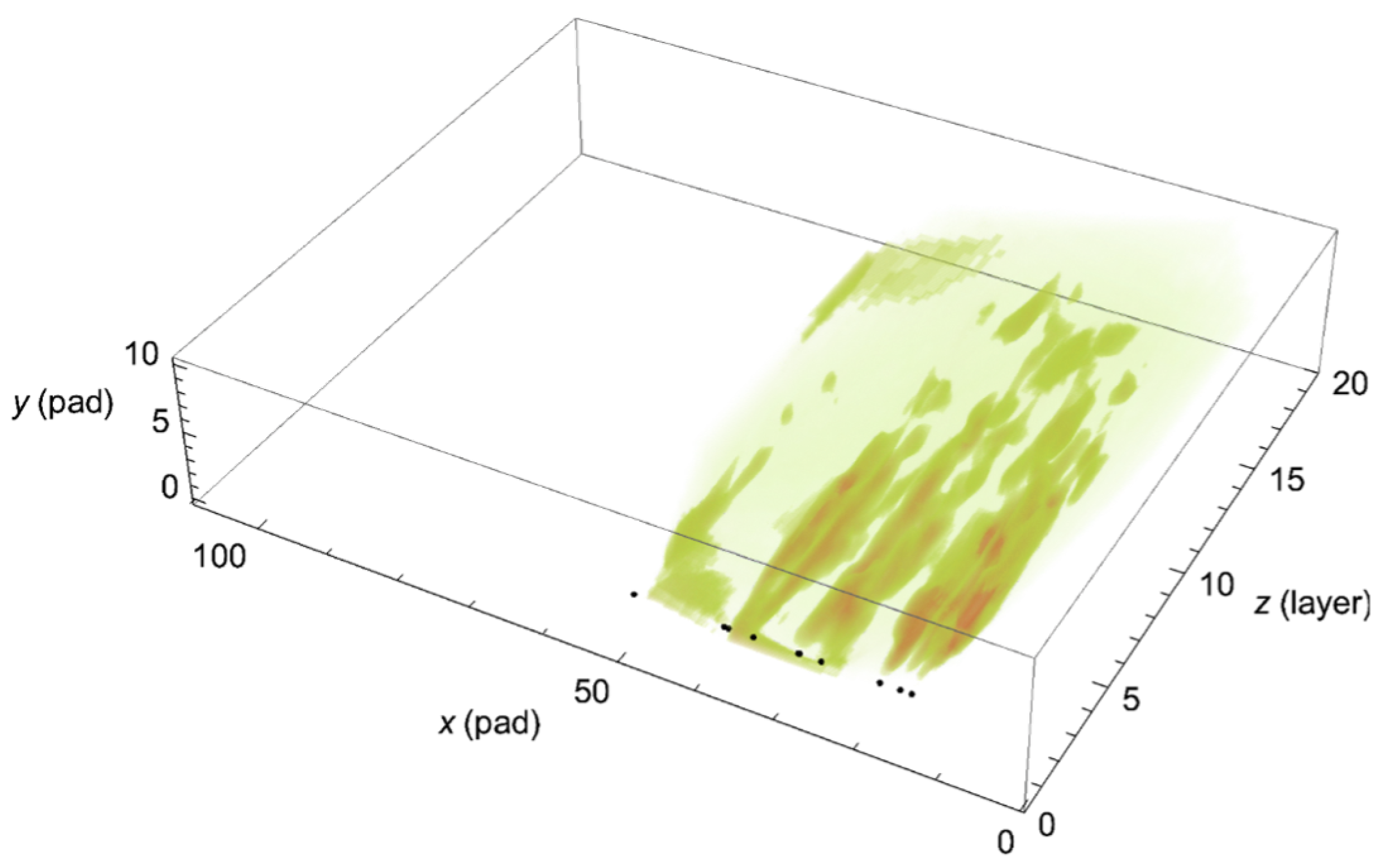
An electromagnetic calorimeter (ECAL) is a detector in HEP based on electromagnetic interactions, including bremsstrahlung and pair creation. Electrons, positrons, and photons can easily create showers inside an ECAL. To obtain a snapshot of the shower, multiple layers of sensitive materials are inserted in an ECAL where the energy of showers is deposited, leading to an image (as in Figure 1) reflecting each event. Monte-Carlo simulations [3] are employed to build these images during the design process. In addition, algorithms for extracting the particle information from the images have to be developed for evaluating the design. It is in this context that we use the deep learning (DL) methodology of a convolutional neural network (CNN) for ECAL information extraction.

Neural networks have been used in HEP for decades [4,5,6,7,8,9,10,11]. Some recent works have also covered shower identification and reconstruction in calorimeters [12,13,14]. Most of the neural network studies in HEP are dedicated to the extraction of weak signals from backgrounds, such as in the discovery of the Higgs boson [15,16]. Here we present an example of the design of an ECAL for the proposed Laser und XFEL Experiment (LUXE) [17]. Designed to account for positron identification in LUXE, the ECAL has a three-dimensional (3D) structure of $(110\times 11\times 20=)$ 24,200 elements of detector pads. This detector is exposed to incoming positrons produced by a laser beam colliding with electrons, and creates an image of energy deposition with the 24K pixels. During the experiment, the positrons will be generated periodically. Each batch of positrons is called an “event”.

The energy distribution and multiplicity of positrons hitting the detector depend on a few factors. Apart from statistical and quantum fluctuations, the physical results of the collision will change along with the properties of the laser beam which, in this case, is qualified by a single parameter: the focal radius of the laser beam. In this paper, samples with radii $\rho =3,5,8$ µm are investigated. In the loosely focusing case ($\rho =8$ µm), we find fewer than three positrons per event. A few couples to tens of positrons reach the ECAL when $\rho =5$ µm. The number of positrons dramatically increases above 100 to a few thousands in the tightly focusing scenario ($\rho =3$ µm). Figure 1 sketches an expected shower structure within the detector. The overlapping of showers in a ten-positron event is clearly visible. The challenges for the LUXE ECAL lie in the identification of positrons from the background, as well as its effectiveness in high-multiplicity events. We will provide an algorithm that translates the readings of the 24K variables to the aforementioned positron properties, and covers the different scenarios with largely various numbers of positrons.

The difficulties of working within such a data-space may be addressed by a deep neural network. In principle, the reading of each event on the detector is assumed to present a 3D image, whose voxels are the pads located at the Cartesian coordinates, and their readouts are regarded as continuous outputs associated with the voxels. Viewed as such, it seems quite natural to employ the methodology of a CNN for our analysis. This methodology has been employed for the task of character recognition [18] and its mechanism involves hierarchical feature abstraction as demonstrated in [19]. An important leap was made by AlexNet [20], which provided the best solution to an automatic classification competition based on ImageNet, a database including 1000 categories of 1000 images each. This started the modern era of deep learning [21] and was soon followed by many other networks.

In this article, we demonstrate the results obtained from a customized version of the successful residual network ResNet10 [22]. We apply this tool to a detector image of 110-by-11-by-20 elements in a 3D Euclidean space with $(x,y,z)$ coordinates. The structure of the neural network will be introduced in Section 2. In Section 3, the outcomes of the neural network will be presented within 1% error from the positron properties in the MC simulations. The robustness of the CNN is further studied in Section 4, and leads to a prospect for a more economic design of the ECAL without losing information.

2. Methods

The neural network computational approach is based on analogy with the neural connectivity in the brain. The convolutions in CNN draw further lessons from the visual system. Having many layers with restricted connectivity patterns, the CNN is supposed to develop feature maps with increased complexity, which are generalized from the patterns on which the CNN is being trained. Our CNN analysis is based on ResNet [22]. It has architectural structures of blocks containing two or three layers and connectivities among non-consecutive layers within the block.

The original ResNet has excelled in analysis of colored images. Its input layer has 2 space dimensions and 1 color dimension containing images in 3 color filters. In our ECAL application, all 3 spatial axes start out as position indices of the detector. The architecture of our CNN is demonstrated in

Table 1. The ResNet10 overall structure, using customary ResNet specifications.

Type	3D Structure	Number of Layers	Number of Features
Input	[110, 11, 21]
Layer 1	[31, 11, 21]	1	64
Block 1	[16, 6, 11]	2	64
Block 2	[8, 3, 6]	3	128
Block 3	[4, 2, 3]	3	256
Block 4	[2, 1, 2]	3	512
Linear		1
Output

, using customary ResNet specifications [23]. A three-dimensional convolution leads to the first layer of a reduced x dimension. Following it are four ResNet blocks containing 2 or 3 layers, which are interconnected via 3D convolutions, with varying numbers of feature map dimensions. The final layer is a linear vector of size 1024 connected to the output. The 14.4 million network parameters are trained by stochastic gradient descent, which uses the ECAL energy readings as inputs and the energies and multiplicity of positrons in the MC simulation as targets (ground truth). The output can be positron multiplicity, a moment of the energy distribution of the shower (Section 3.1), or the discrete energy spectrum consisting of an array of histogram bins (Section 3.2). The open-source code employed for our calculations is provided in GitHub [24].

3. Positron Multiplicity and Energy Distribution

An ideal detector output would be a list of energies for the particles generated in each event, leading to the energy distribution function $f\left(E\right)$ in

$${n|}_{E_1}^{E_2}={\int }_{E_1}^{E_2}f\left(E\right)\mathrm{d}E.$$

(1)

The number of positrons with energies in between $E_1$ and $E_2$ is denoted by ${n|}_{E_1}^{E_2}$. Obviously, the multiplicity n is the integral when $-E_1$ and $E_2$ are set to positive infinity. The average energy distribution function is characterized by the focal radius $\rho$ of the laser.

Following this section, two aspects of $f\left(E\right)$ will be studied using our CNN methodology, one based on moments and the other on histograms of the distribution.

3.1. Multiplicity and Distribution Moments

The i-th moment of a continuous distribution is defined by

$$M_i=〈E^i〉=\int E^{i}f\left(E\right)\mathrm{d}E.$$

(2)

In each event (labeled a), a finite number of positrons is generated. It serves as a sample of the distribution, which we try to characterize. Naturally, this number $n\left(a\right)$ varies among events. Both the multiplicity $n\left(a\right)$ and the various discrete moments $m_i\left(a\right)$ are calculated from the MC simulation, and are associated with the ECAL’s energy deposition images. Characteristically, we are interested in the first few moments. The CNN is trained on a randomly chosen 75% of the dataset with one event at a time, and tested on the remaining 25%. Different CNNs are used to train for $n\left(a\right)$ and each one of the energy moments $m_i\left(a\right)$. 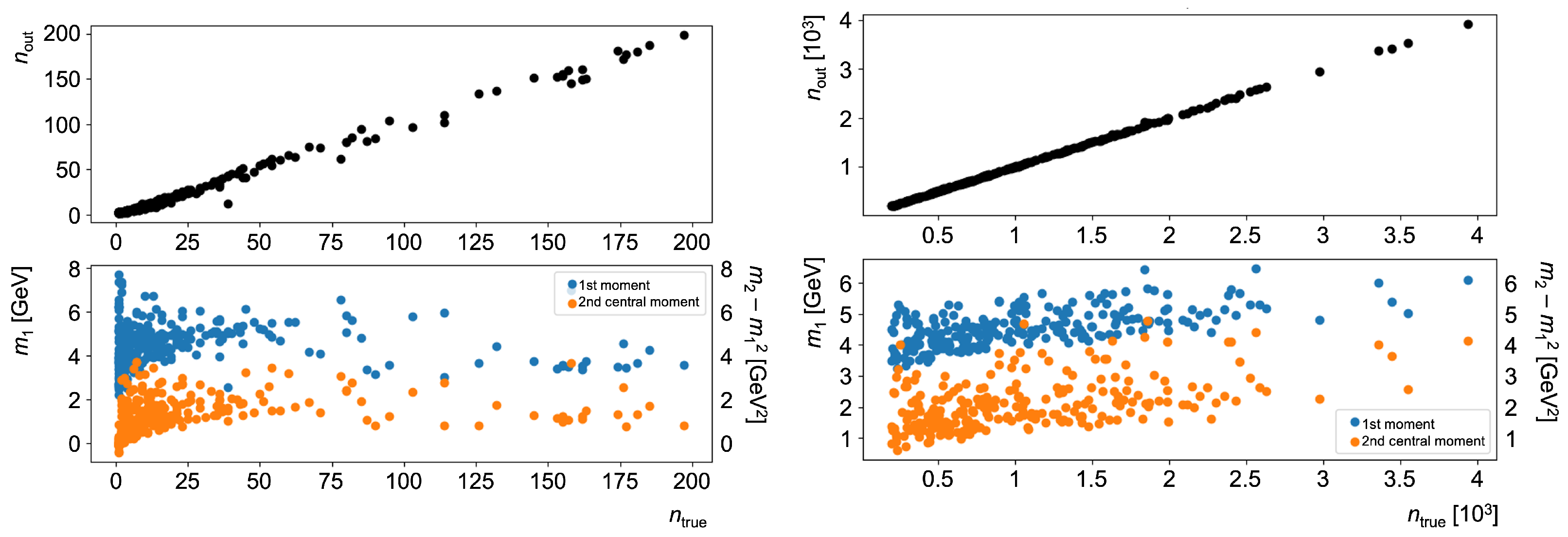The results of the multiplicity and first two central moments are displayed in Figure 2.

In

Table 2. Moments of the energy distribution of the test set of the $\rho =3$ µm source, summing over all events. The true values are determined from the MC data, and the reconstructed values arise from the CNN evaluation of the ECAL analysis of individual events, as described above.

Moments	True Value	Output	Bias
$M_1\left[\mathrm{GeV}\right]$	4.65	4.71	1.2%
$M_2\left[{\mathrm{GeV}}^2\right]$	24.1	24.6	2.3%
$M_3\left[{\mathrm{GeV}}^3\right]$	137.4	142.8	3.9%

, with the discrete moments of each event, the overall moments for the dataset can be estimated via weighted average, using the multiplicity of each event as the weight

$$M_i=\sum _a\frac{n\left(a\right)m_i\left(a\right)}{N}\mathrm{where}N=\sum _{a}n\left(a\right).$$

(3)

3.2. Discrete Positron Energy Spectrum

Apart from the characteristic parameters of the distribution, another straightforward method is often used by breaking apart the continuous distribution function into a discrete histogram like Equation (1). We train and test the energy spectrum in terms of a histogram with 20 bins. The energy ranges of these bins are predetermined as $\left[E_j,E_{j+1}\right)$ and

$$E_{j+1}=E_j+0.7\mathrm{GeV},E_0=0$$

(4)

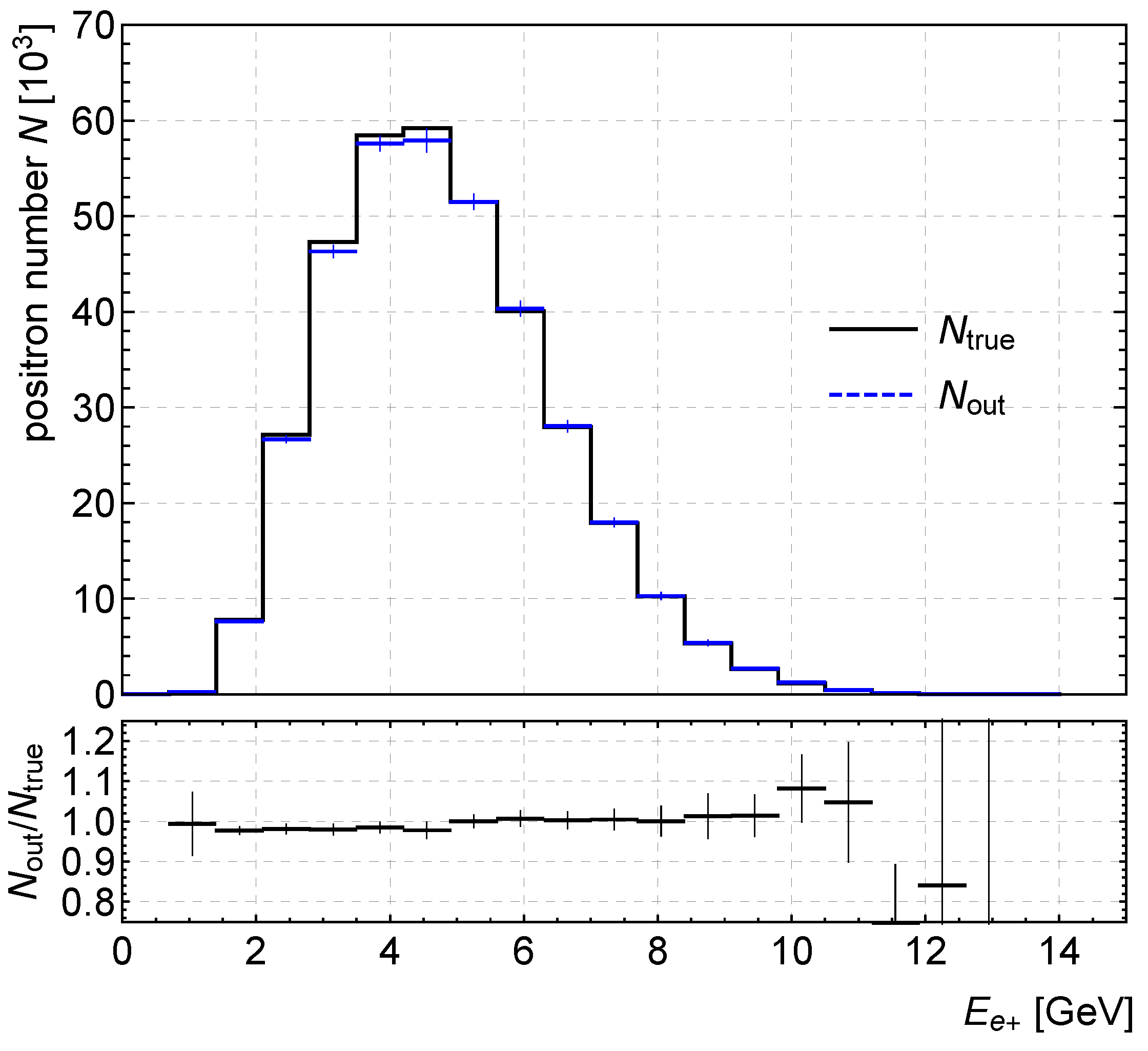
where j is the bin number. The analysis is carried out by associating each event with an array of 20 entries, corresponding to the histograms of ${n|}_{E_j}^{E^{j+1}}$ with $j=0,1,\dots ,19$. Employing the $\rho =3$ µm data, we generated 10 random runs (65% train and 35% test out of 1000 events in each run) and evaluated their histograms. The average true (MC) results were compared to the CNN outputs of the average test set results, shown in Figure 3.

The CNN predictions have a small average bias over all bins $〈\Delta N〉/N_{\mathrm{true}}=-(0.88\pm 0.42)\%$ and its root-mean-square is $\sqrt{〈\Delta N^2〉}/N_{\mathrm{true}}=(0.92\pm 0.25)\%$, where $\Delta N=N_{\mathrm{out}}-N_{\mathrm{true}}$. The average number of positrons per event in these 10 runs was $1024\pm 31$ for the training and $1000\pm 46$ for the test data.

Another estimate of the accuracy of a histogram prediction is the conventional KL distance [25]

$$\mathrm{KL}(P,Q)=\sum _j{p}_{j}log(p_j/q_j)$$

(5)

as the metric for the closeness of two probability distributions P and Q. Here $p_j,q_j$ are, respectively, the probabilities defined as $p_j=N_{\mathrm{true},j}/N_{\mathrm{true}}$ and $q_j=N_{\mathrm{out},j}/N_{\mathrm{out}}$ for the 20 bins. The KL distance for the Figure 3 distributions is $1.2\times {10}^{-4}$ indicating that the true distribution is in agreement with the CNN output.

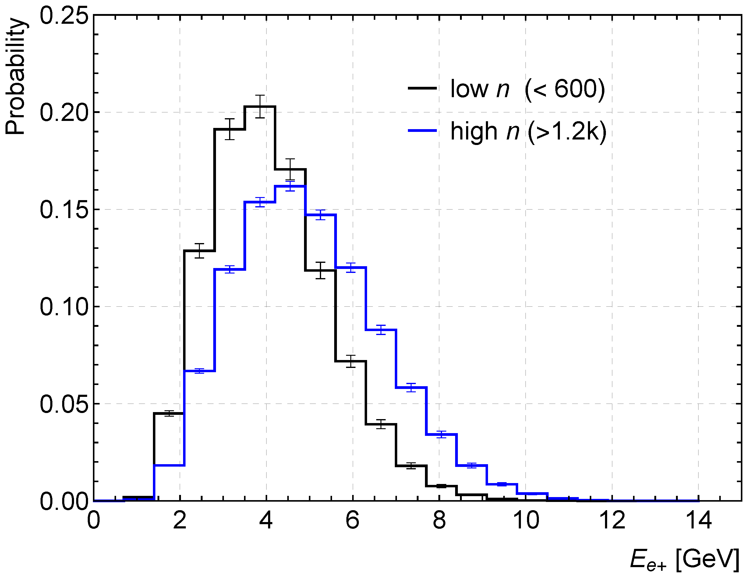
It should be noted that the reconstruction of the test-set distributions by the CNN has been performed through accumulating the data event by event. This means that all events construct harmoniously a coherent distribution, even though the histograms differ from event to event. In this dataset, as the multiplicity of an event increases, so does its average energy (near the peak position of the histogram). This can be seen in Figure 2, and is also demonstrated in Figure 4, where we plot histograms of the lowest range and of the highest range of n for $\rho =3$ µm events.

Trying to generalize from the $\rho =3$ µm CNN, and applying it to $\rho =5$ µm test data, we have to carefully adjust the energy ranges accordingly. With this aspect being taken into account, the generalization works very well. This point is important when we consider future applications to real-world experimental data, where we have to select reliable MC datasets for training procedures.

4. The Detector-Network System

In this section, we are going to test the robustness and characteristics of neural networks that are shaped during the training process. An event is recorded by the detector through signals produced by its 24,200 elements. This event may be regarded as a point in a 24K-dimensional phase space. A few events with the same characteristics, e.g., the same number of positrons n, must occur in the same neighborhood in this large space. Otherwise, learning the number of positrons by the CNN is impossible; learning implies that all points in this neighborhood be given the same label. Only then can the procedure be generalized, and the label can be applied to a test event that appears in the same neighborhood. The fact that all events with the same labeling end up in the same neighborhood is important because predicting n is only successful when these labels are attached to the particular neighborhood by the training procedure of the CNN. This neighborhood can have multiple regions, as long as these regions are not shared with events of different characteristics.

For this to happen, the dynamics should be robust and non-chaotic, i.e., small changes in initial conditions should not lead to large changes of the final region in both the detector phase-space and its representation in the network. This can also be stated as the condition that clusters of data representing different n values should be well separated within the CNN.

To demonstrate what happens in our analysis, we look for the property of compositionality in the CNN, as well as the variation of outputs by depriving the training of unnecessary information. The testing result shows a possibility of improving the design of ECAL.

4.1. Compositionality of CNN Prediction

We use the predictability of n as a connection between the CNN representation and the proximity and order properties of integers, in order to establish an intuitive answer. In particular, a question of compositionality is presented: given two detector images, a and b, will their superposition $a+b$ in the CNN detector-image input lead to $n(a+b)=n\left(a\right)+n\left(b\right)$? To perform this test, we train the CNN in the regular fashion, and apply it to a test set which is generalized to include such combinations. The superposition of two images is defined as the sum of all their detector readings, and may be evaluated by the CNN that was trained to predict n of single images. We tested this question using the $\rho =5$ µm data. Intermediate n values of $20<n<200$ show that approximate compositionality holds. 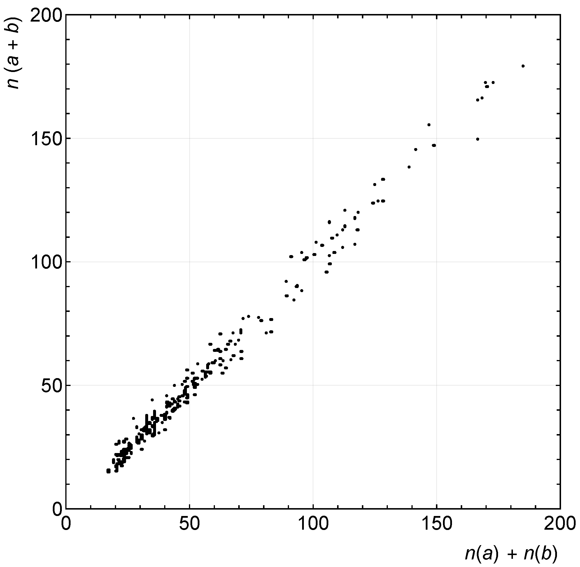The results are displayed in Figure 5. The points in these plots correspond to non-recurrent choices of $(a,b)$ pairs, for which the network estimation $n(a+b)$ is plotted vs. the known sum of $n\left(a\right)+n\left(b\right)$. Although the order of events does not adhere to a strict chain of integers, these data hint that the detector-network system is not very far from it in the shown range of n values.

4.2. Information Reduction

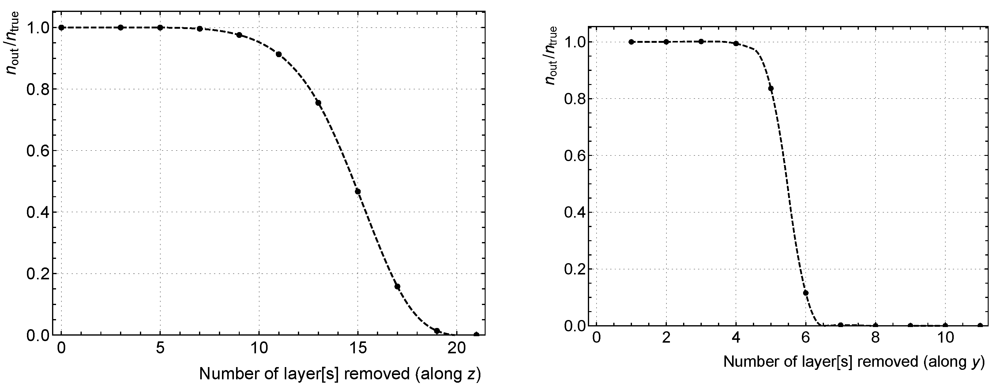
Here we turn to an analysis of the way events occupy the 24K parameter space of the detector. By employing the CNN, it is easy to test the information derived from different layers of the detector. During our train/test procedure, we remove, in the test set only, layers from the detector image in the z-direction (starting with its last layer) or in the y-direction (starting from the top). The results for changes in the estimated multiplicity are displayed in Figure 6. In the z-direction we find that the last 10 layers (out of 21) have negligible impact, and most of the n information is carried by the first 4–6 z-layers. Similar trends are observed for the prediction of the average energy. That is to say, the CNN does not rely on the information from a large number of the detector elements. This raises the interesting possibility that we may analyze the data by considering a reduced detector image, which we proceed to do by using only three y-layers ($y=4,5,6$) and the first 10 z-layers.

The resulting energy histograms are very similar, both in shape and in quality, to the ones obtained based on the full detector image. The bias values are of order 1 to 2%. Note that this is achieved in a strongly reduced parameter space, using only 3K elements out of the whole 24K of the detector.

5. Conclusions

Our study exemplifies the importance of supplying a hardware system, such as an electromagnetic calorimeter in high energy physics, with interpreter software, represented by a deep network. Whereas the detector has a large number of outgoing signals, the network has a much larger number of parameters that can trivially embed the results of the detector. The non-trivial results of the deep learning architecture of the ResNet10 model demonstrate that after 50 training epochs, this embedding leads to retrievable results on the test sets, allowing us to capture the physical properties of the events that we study.

The combined detector-network system is somewhat analogous to the visual system, with the detector playing the role of the eye and the network being the analog of the visual cortex. The well-trained neural networks give an average bias of $-0.88\%$ with an RMS of 0.92%. The success of the CNN lies in the correct and robust identification of the data space neighborhood that a queried event belongs to.

Moreover, since the network starts out with an image of the detector output, we can easily find out which are the important elements of the detector. By removing layers from the detector image, we conclude that in the problem at hand we can, using the CNN, retrieve all the physical information we have studied from an image reduced by a factor of 8. This is an important conclusion that should be taken into account during the design of the detector. Thus, the power of CNN software can be harnessed for efficient hardware design and data extraction needed for high energy physics experiments.

Finally, we wish to comment on our modeling procedure. The conventional approach in HEP is to model the development of showers in the detector by a branching process based on the expected interactions of the particles at each interaction point in the detector. Our suggestion is to confront this rule-based approach with an inference-based one, relying on CNN analysis. The latter is validated by a train/test procedure that does not depend on detailed understanding (although it can benefit from it). If its results turn out to have lower prediction errors than the rule-based approach, it should be preferred once it passes all tests, because it is the statistically sound decision. Conceptually, this approach shares with Zero Knowledge Proof [26], a well-known concept in cryptography, the understanding that one does not need to comprehend the details of an algorithm in order to be convinced of its validity.