1. Introduction
The Euclidean expected value can be generalized to geometric spaces in several ways. Fréchet [
1] generalized the notion of mean values to arbitrary metric spaces as minimizers of the sum of squared distances. Fréchet’s notion of mean values therefore naturally includes means on Riemannian manifolds. On manifolds without metric, for example, affine connection spaces, a notion of the mean can be defined by exponential barycenters, see, e.g., [
2,
3]. Recently, Hansen et al. [
4,
5] introduced a probabilistic notion of a mean, the diffusion mean. The diffusion mean is defined as the most likely starting point of a Brownian motion given the observed data. The variance of the data is here modelled in the evaluation time
of the Brownian motion, and Varadhan’s asymptotic formula relating the heat kernel with the Riemannian distance relates the diffusion mean and the Fréchet mean in the
limit.
Computing sample estimators of geometric means is often difficult in practice. For example, estimating the Fréchet mean often requires evaluating the distance to each sample point at each step of an iterative optimization to find the optimal value. When closed-form solutions of geodesics are not available, the distances are themselves evaluated by minimizing over curves ending at the data points, thus leading to a nested optimization problem. This is generally a challenge in geometric statistics, the statistical analysis of geometric data. However, it can pose an even greater challenge in geometric deep learning, where a weighted version of the Fréchet mean is used to define a generalization of the Euclidean convolution taking values in a manifold [
6]. As the mean appears in each layer of the network, closed-form geodesics is in practice required for its evaluation to be sufficiently efficient.
As an alternative to the weighted Fréchet mean, Ref. [
7] introduced a corresponding weighted version of the diffusion mean. Estimating the diffusion mean usually requires ability to evaluate the heat kernel making it often similarly computational difficult to estimate. However, Ref. [
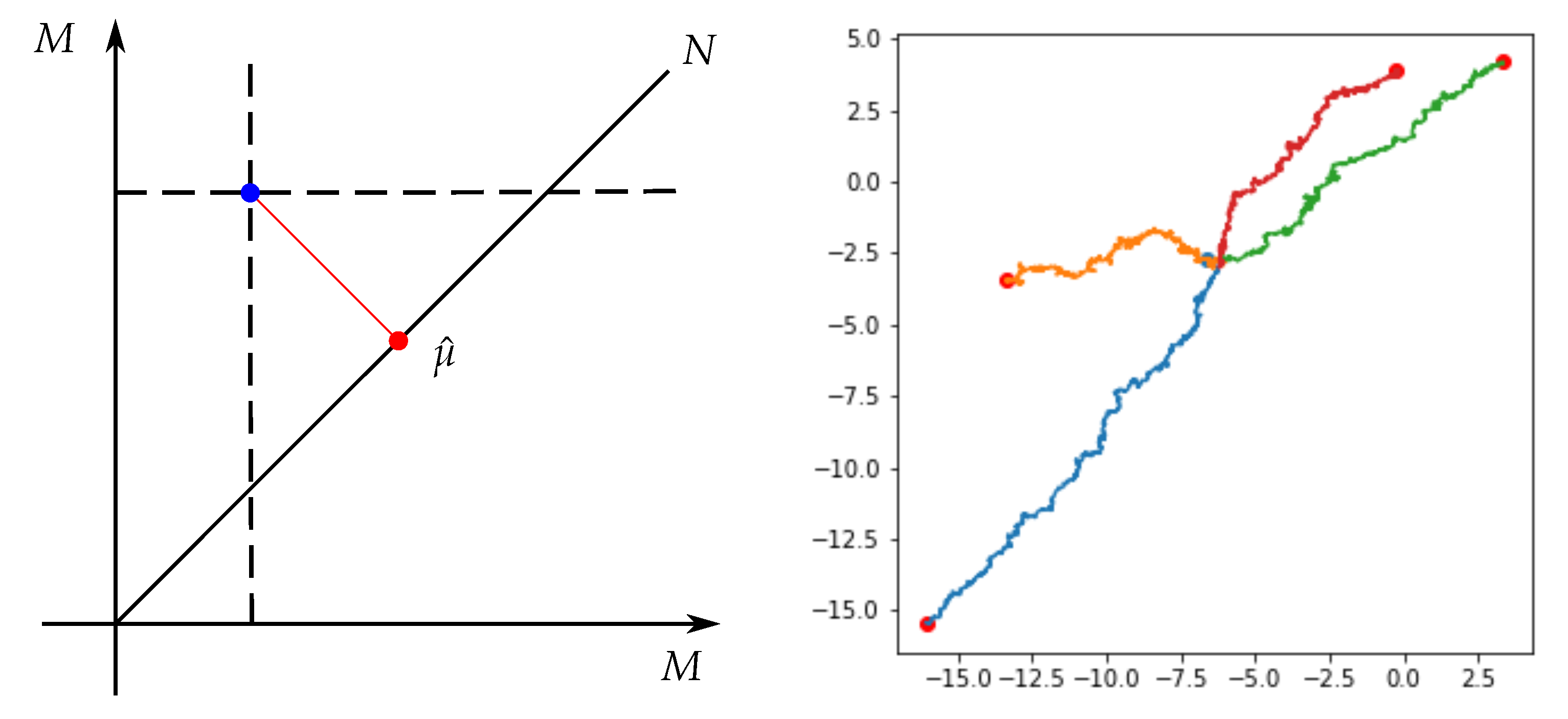
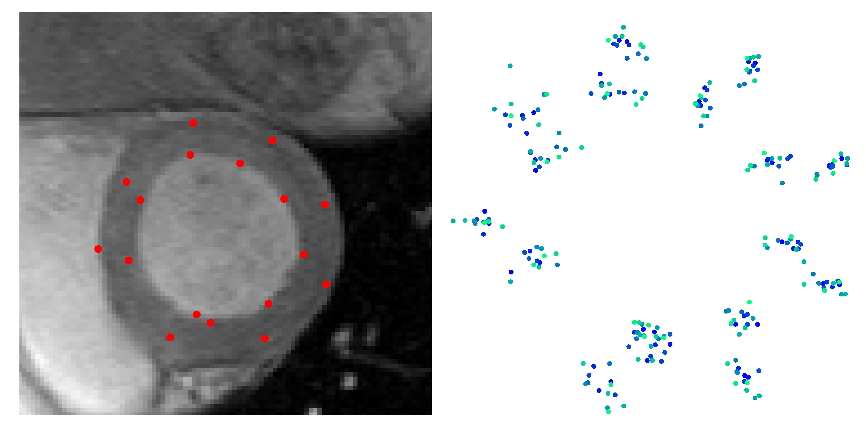
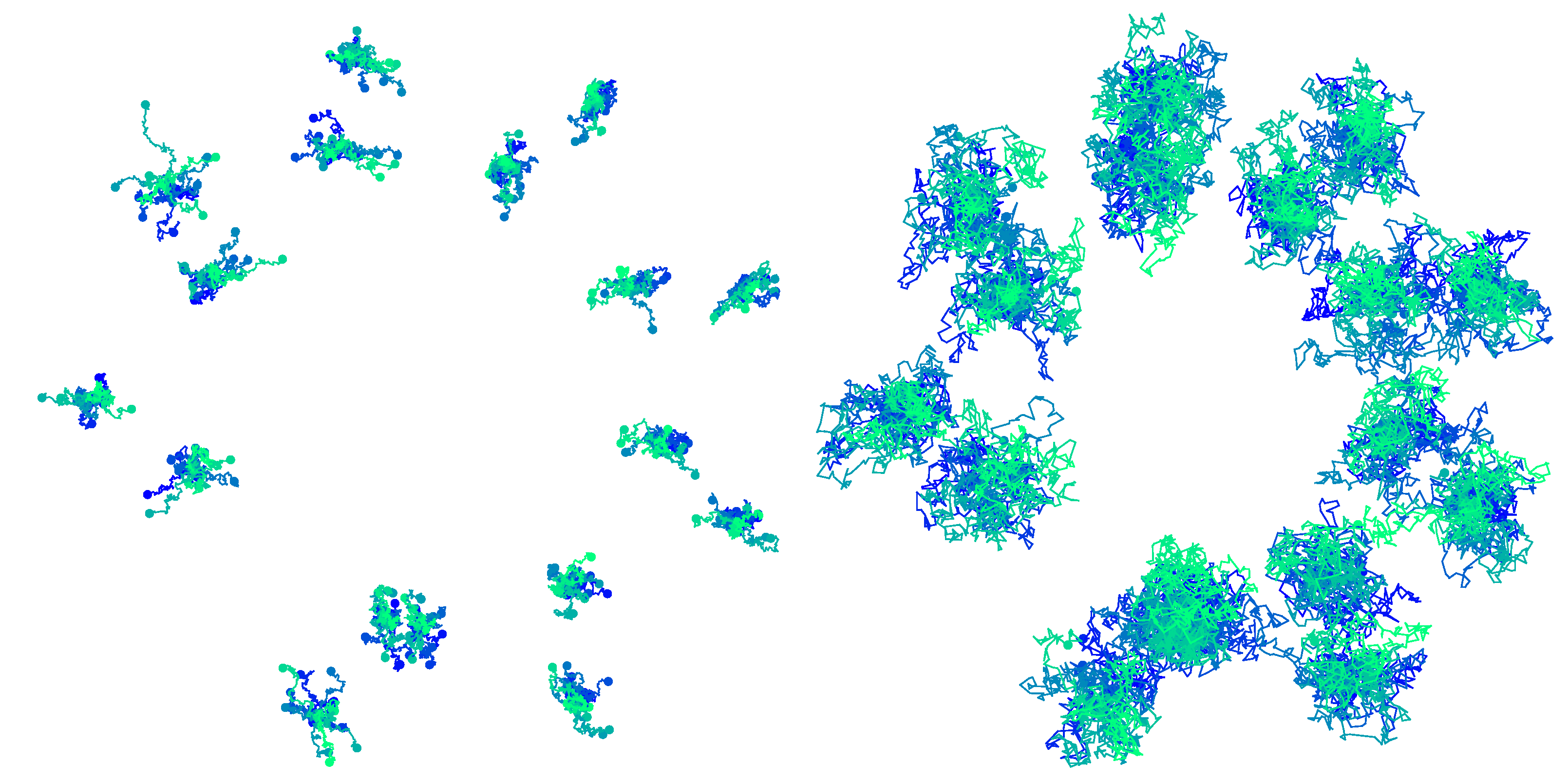
7] also sketched a simulation-based approach for estimating the (weighted) diffusion mean that avoids numerical optimization and estimation of the heat kernel. Here, a mean candidate is generated by simulating a single forward pass of a Brownian motion on a product manifold conditioned to hit the diagonal of the product space. The idea is sketched for samples in
in
Figure 1.
Contribution
In this paper, we present a comprehensive investigation of the simulation-based mean sampling approach. We provide the necessary theoretical background and results for the construction, we present two separate simulation schemes, and we demonstrate how the schemes can be used to compute means on high-dimensional manifolds.
2. Background
We here outline the necessary concepts from Riemannian geometry, geometric statistics, stochastic analysis, and bridge sampling necessary for the sampling schemes presented later in the paper.
2.1. Riemannian Geometry
A Riemannian metric g on a d-dimensional differentiable manifold M is a family of inner products on each tangent space varying smoothly in p. The Riemannian metric allows for geometric definitions of, e.g., length of curves, angles of intersections, and volumes on manifolds. A differentiable curve on M is a map for which the time derivative belongs to , for each . The length of the differentiable curve can then be determined from the Riemannian metric by . Let and let be the set of differentiable curves joining p and q, i.e., and . The (Riemannian) distance between p and q is defined as . Minimizing curves are called geodesics.
A manifold can be parameterized using coordinate charts. The charts consist of open subsets of
M providing a global cover of
M such that each subset is diffeomorphic to an open subset of
, or, equivalently,
itself. The exponential normal chart is often a convenient choice to parameterize a manifold for computational purposes. The exponential chart is related to the exponential map
that for each
is given by
, where
is the unique geodesic satisfying
and
. For each
, the exponential map is a diffeomorphism from a star-shaped subset
V centered at the origin of
to its image
, covering all
M except for a subset of (Riemannian) volume measure zero,
, the cut-locus of
p. The inverse map
provides a local parameterization of
M due to the isomorphism between
and
. For submanifolds
, the cut-locus
is defined in a fashion similar to
, see e.g., [
8].
Stochastic differential equations on manifolds are often conveniently expressed using the frame bundle , the fiber bundle which for each point assigns a frame or basis for the tangent space , i.e., consists of a collection of pairs , where is a linear isomorphism. We let denote the projection . There exist a subbundle of consisting of orthonormal frames called the orthonormal frame bundle . In this case, the map is a linear isometry.
2.2. Weighted Fréchet Mean
The Euclidean mean has three defining properties: The
algebraic property states the uniqueness of the arithmetic mean as the mean with residuals summing to zero, the
geometric property defines the mean as the point that minimizes the variance, and the
probabilistic property adheres to a maximum likelihood principle given an i.i.d. assumption on the observations (see also [
9] Chapter 2). Direct generalization of the arithmetic mean to non-linear spaces is not possible due to the lack of vector space structure. However, the properties above allow giving candidate definitions of mean values in non-linear spaces.
The Fréchet mean [
1] uses the geometric property by generalizing the mean-squared distance minimization property to general metric spaces. Given a random variable
X on a metric space
, the Fréchet mean is defined by
In the present context, the metric space is a Riemannian manifold
M with Riemannian distance function
d. Given realizations
from a distribution on
M, the estimator of the weighted Fréchet mean is defined as
where
are the corresponding weights satisfying
and
. When the weights are identical, (
2) is an estimator of the Fréchet mean. Throughout, we shall make no distinction between the estimator and the Fréchet mean and will refer to both as the Fréchet mean.
In [
6,
10], the weighted Fréchet mean was used to define a generalization of the Euclidean convolution to manifold-valued inputs. When closed-form solutions of geodesics are available, the weighted Fréchet mean can be estimated efficiently with a recursive algorithm, also denoted an inductive estimator [
6].
2.3. Weighted Diffusion Mean
The diffusion mean [
4,
5] was introduced as a geometric mean satisfying the probabilistic property of the Euclidean expected value, specifically as the starting point of a Brownian motion that is most likely given observed data. This results in the diffusion
t-mean definition
where
denotes the transition density of a Brownian motion on
M. Equivalently,
denotes the solution to the heat equation
, where
denotes the Laplace-Beltrami operator associated with the Riemannian metric. The definition allows for an interpretation of the mean as an extension of the Fréchet mean due to Varadhan’s result stating that
uniformly on compact sets disjoint from the cut-locus of either
x or
y [
11].
Just as the Fréchet mean, the diffusion mean has a weighted version, and the corresponding estimator of the weighted diffusion
t-mean is given as
Please note that the evaluation time is here scaled by the weights. This is equivalent to scaling the variance of the steps of the Brownian motion [
12].
As closed-form expressions for the heat kernel are only available on specific manifolds, evaluating the diffusion
t-mean often rely on numerical methods. One example of this is using bridge sampling to numerically estimate the transition density [
9,
13]. If a global coordinate chart is available, the transition density can be written in the form (see [
14,
15])
where
g is the metric matrix,
a a square root of
g, and
denotes the correction factor between the law of the true diffusion bridge and the law of the simulation scheme. The expectation over the correction factor can be numerically approximated using Monte Carlo sampling. The correction factor will appear again when we discuss guided bridge proposals below.
2.4. Diffusion Bridges
The proposed sampling scheme for the (weighted) diffusion mean builds on simulation methods for conditioned diffusion processes, diffusion bridges. Here, we outline ways to simulate conditioned diffusion processes numerically in both the Euclidean and manifold context.
Euclidean Diffusion Bridges
Let
be a filtered probability space, and
X a
d-dimensional Euclidean diffusion
satisfying the stochastic differential equation (SDE)
where
W is a
d-dimensional Brownian motion. Let
be a fixed point. Conditioning
X on reaching
v at a fixed time
gives the bridge process
. Denoting this process
Y, Doob’s
h-transform shows that
Y is a solution of the SDE (see e.g., [
16])
where
denotes the transition density of the diffusion
X,
, and where
is a
d-dimensional Brownian motion under a changed probability law. From a numerical viewpoint, in most cases, the transition density is intractable and therefore direct simulation of (
7) is not possible.
If we instead consider a Girsanov transformation of measures to obtain the system (see, e.g., [
17] Theorem 1)
the corresponding change of measure is given by
From (
7), it is evident that
gives the diffusion bridge. However, different choices of the function
h can yield processes which are absolutely continuous regarding the actual bridges, but which can be simulated directly.
Delyon and Hu [
17] suggested to use
, where
q denotes the transition density of a standard Brownian motion with mean
v, i.e.,
. They furthermore proposed a method that would disregard the drift term
b, i.e.,
. Under certain regularity assumptions on
b and
, the resulting processes converge to the target in the sense that
a.s. In addition, for bounded continuous functions
f, the conditional expectation is given by
where
is a functional of the whole path
Y on
that can be computed directly. From the construction of the
h-function, it can be seen that the missing drift term is accounted for in the correction factor
.
The simulation approach of [
17] can be improved by the simulation scheme introduced by Schauer et al. [
18]. Here, an
h-function defined by
is suggested, where
denotes the transition density of an auxiliary diffusion process with known transition densities. The auxiliary process can for example be linear because closed-form solutions of transition densities for linear processes are available. Under the appropriate measure
, the guided proposal process is a solution to
Note the factor
in the drift in (
7) which is also present in (
11) but not with the scheme proposed by [
17]. Moreover, the choice of a linear process grants freedom to model. For other choices of an
h-functions see e.g., [
19,
20].
Marchand [
19] extended the ideas of Delyon and Hu by conditioning a diffusion process on partial observations at a finite collection of deterministic times. Where Delyon and Hu considered the guided diffusion processes satisfying the SDE
for
over the time interval
, Marchand proposed the guided diffusion process conditioned on partial observations
solving the SDE
where
is be any vector satisfying
,
a deterministic matrix in
whose
rows form a orthonormal family,
are projections to the range of
, and
. The
only allow the application of the guiding term on a part of the time intervals
. We will only consider the case
. The scheme allows the sampling of bridges conditioned on
.
2.5. Manifold Diffusion Processes
To work with diffusion bridges and guided proposals on manifolds, we will first need to consider the Eells–Elworthy–Malliavin construction of Brownian motion and the connected characterization of semimartingales [
21]. Endowing the frame bundle
with a connection allows splitting the tangent bundle
into a horizontal and vertical part. If the connection on
is a lift of a connection on
M, e.g., the Levi–Civita connection of a metric on
M, the horizontal part of the frame bundle is in one-to-one correspondence with
M. In addition, there exist fundamental horizontal vector fields
such that for any continuous
-valued semimartingale
Z the process
U defined by
is a horizontal frame bundle semimartingale, where ∘ denotes integration in the Stratonovich sense. The process
is then a semimartingale on
M. Any semimartingale
on
M has this relation to a Euclidean semimartingale
.
is denoted the development of
, and
the antidevelopment of
. We will use this relation when working with bridges on manifolds below.
When
is a Euclidean Brownian motion, the development
is a Brownian motion. We can in this case also consider coordinate representations of the process. With an atlas
of
M, there exists an increasing sequence of predictable stopping times
such that on each stochastic interval
the process
, for some
(see [
22] Lemma 3.5). Thus, the Brownian motion
x on
M can be described locally in a chart
as the solution to the system of SDEs, for
where
denotes the matrix square root of the inverse of the Riemannian metric tensor
and
is the contraction over the Christoffel symbols (see, e.g., [
11] Chapter 3). Strictly speaking, the solution of Equation (
15) is defined by
.
We thus have two concrete SDEs for the Brownian motion in play: The
SDE (
14) and the coordinate SDE (
15).
Throughout the paper, we assume that M is stochastically complete, i.e., the Brownian motions does not explode in finite time and, consequently, , for all and all .
2.6. Manifold Bridges
The Brownian bridge process Y on M conditioned at is a Markov process with generator . Closed-form expressions of the transition density of a Brownian motion are available on selected manifolds including Euclidean spaces, hyperbolic spaces, and hyperspheres. Direct simulation of Brownian bridges is therefore possible in these cases. However, generally, transition densities are intractable and auxiliary processes are needed to sample from the desired conditional distributions.
To this extent, various types of bridge processes on Riemannian manifolds have been described in the literature. In the case of manifolds with a pole, i.e., the existence of a point
such that the exponential map
is a diffeomorphism, the
semi-classical (Riemannian Brownian) bridge was introduced by Elworthy and Truman [
23] as the process with generator
, where
and
denotes the Jacobian determinant of the exponential map at
v. Elworthy and Truman used the semi-classical bridge to obtain heat-kernel estimates, and the semi-classical bridge has been studied by various others [
24,
25].
By Varadhan’s result (see [
11] Theorem 5.2.1), as
, we have the asymptotic relation
. In particular, the following asymptotic relation was shown to hold by Malliavin, Stroock, and Turetsky [
26,
27]:
. From these results, the generators of the Brownian bridge and the semi-classical bridge differ in the limit by a factor of
. However, under a certain boundedness condition, the two processes can be shown to be identical under a changed probability measure [
8] Theorem 4.3.1.
To generalize the heat-kernel estimates of Elworthy and Truman, Thompson [
8,
28] considered the
Fermi bridge process conditioned to arrive in a submanifold
at time
. The Fermi bridge is defined as the diffusion process with generator
, where
For both bridge processes, when
and
N is a point, both the semi-classical bridge and the Fermi bridge agree with the Euclidean Brownian bridge.
Ref. [
15] introduce a numerical simulation scheme for conditioned diffusions on Riemannian manifolds, which generalize the method by Delyon and Hu [
17]. The guiding term used is identical to the guiding term of the Fermi bridge when the submanifold is a single point
v.
3. Diffusion Mean Estimation
The standard setup for diffusion mean estimation described in the literature (e.g., [
13]) is as follows: Given a set of observations
, for each observation
, sample a guided bridge process approximating the bridge
with starting point
. The expectation over the correction factors can be computed from the samples, and the transition density can be evaluated using (
5). An iterative maximum likelihood approach using gradient descent to update
yielding an approximation of the diffusion mean in the final value of
. The computation of the diffusion mean, in the sense just described, is, similarly to the Fréchet mean, computationally expensive.
We here explore the idea first put forth in [
7]: We turn the situation around to simulate
n independent Brownian motions starting at each of
, and we condition the
n processes to coincide at time
T. We will show that the value
is an estimator of the diffusion mean. By introducing weights in the conditioning, we can similarly estimate the weighted diffusion mean. The construction can concisely be described as a single Brownian motion on the
n-times product manifold
conditioned to hit the diagonal
. To shorten notation, we denote the diagonal submanifold
N below. We start with examples with
M Euclidean to motivate the construction.
Example 1. Consider the two-dimensional Euclidean multivariate normal distributionThe conditional distribution of X given follows a univariate normal distributionThis can be seen from the fact that if then for any linear transformation . Defining the random variable , the result applied to gives . The conclusion then follows from . Please note that X and Y are independent if and only if and the conditioned random variable is in this case identical in law to X. Let now be observations and let be an element of the n-product manifold with the product Riemannian metric. We again first consider the case :
Example 2. Let be independent random variables. The conditional distribution is normal . This can be seen inductively: The conditioned random variable is identical to . Now let and and refer to Example 1. To conclude, assume follows the desired normal distribution. Then is normally distributed with the desired parameters and is identical to .
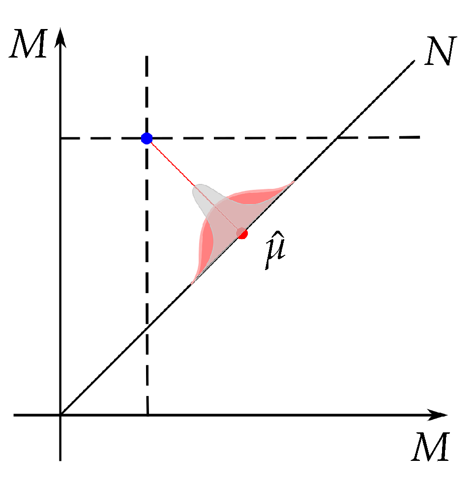
The following example establishes the weighted average as a projection onto the diagonal.
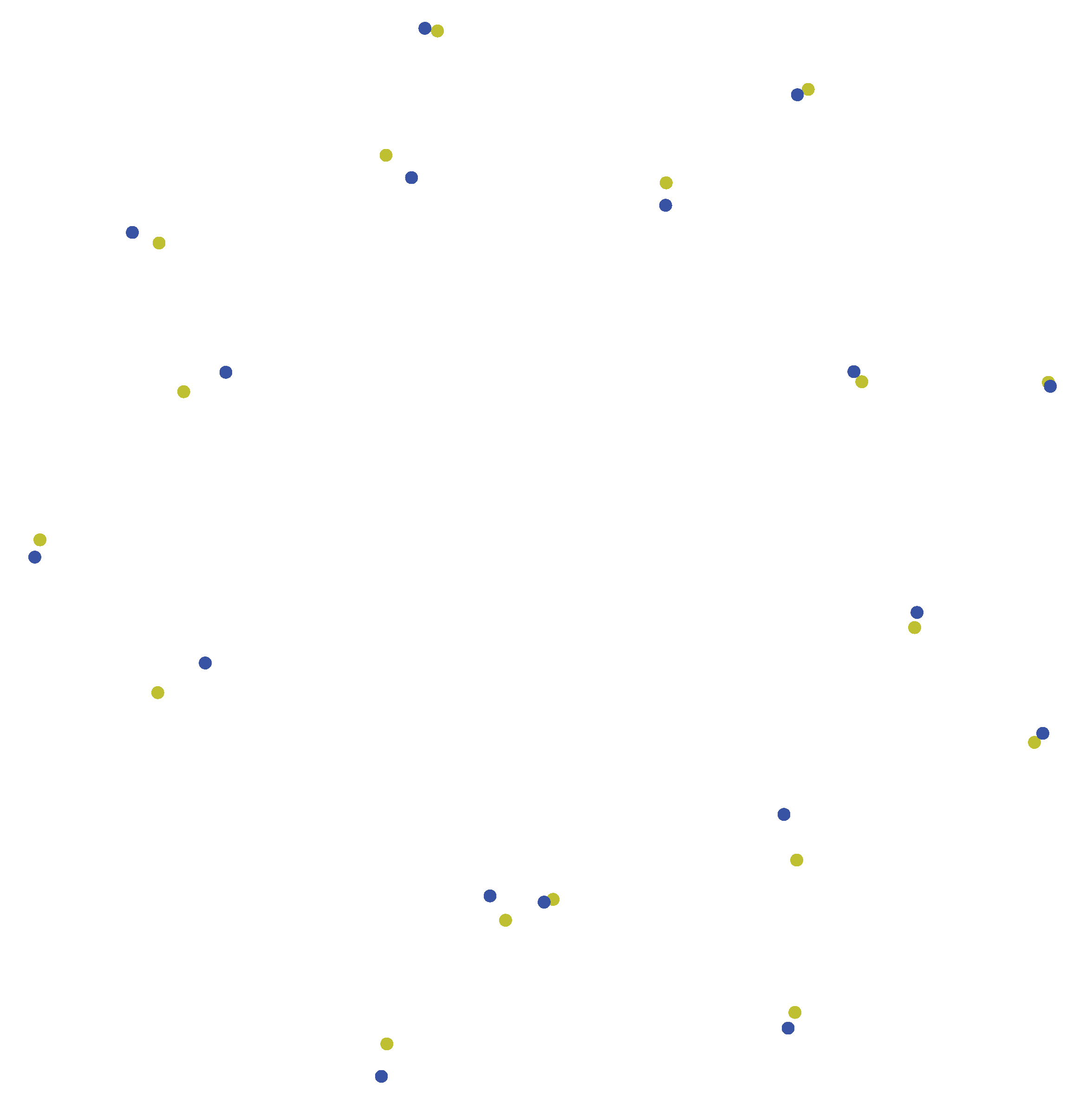
Example 3. Let x be a point in and let P be the orthogonal projection to the diagonal of such that . We see that the projection yields n copies of the arithmetic mean of the coordinates. This is illustrated in Figure 2. The idea of conditioning diffusion bridge processes on the diagonal of a product manifold originates from the facts established in Examples 1–3. We sample the mean by sampling from the conditional distribution from Example 2 using a guided proposal scheme on the product manifolds and on each step of the sampling projecting to the diagonal as in Example 3.
Turning now to the manifold situation, we replace the normal distributions with mean
and variance
with Brownian motions started at
and evaluated at time
. Please note that the Brownian motion density, the heat kernel, is symmetric in its coordinates:
. We will work with multiple process and indicate with superscript the density with respect to a particular process, e.g.,
. Note also that change of the evaluation time
T is equal to scaling the variance, i.e.,
where
is a Brownian motion with variance of the increments scaled by
. This gives the following theorem, first stated in [
7] with sketch proof:
Theorem 1. Let consist of n independent Brownian motions on M with variance and , and let the law of the conditioned process , . Let v be the random variable . Then v has density and for all i a.s. (almost surely).
Proof. because the processes are independent. By symmetry of the Brownian motion and the time rescaling property, . For elements and , . As a result of the conditioning, . In combination, this establishes the result. □
Consequently, the set of modes of equal the set of the maximizers for the likelihood and thus the weighted diffusion mean. This result is the basis for the sampling scheme. Intuitively, if the distribution of v is relatively well behaved (e.g., close to normal), a sample from v will be close to a weighted diffusion mean with high probability.
In practice, however, we cannot sample directly. Instead, we will below use guided proposal schemes resulting in processes with law that we can actually sample and that under certain assumptions, will be absolutely continuous with respect to with explicitly computable likelihood ratio so that .
Corollary 1. Let be the law of and φ be the corresponding correction factor of the guiding scheme. Let be the random variable with law . Then has density .
We now proceed to actually construct the guided sampling schemes.
3.1. Fermi Bridges to the Diagonal
Consider a Brownian motion
in the product manifold
conditioned on
or, equivalently,
,
. Since
N is a submanifold of
, the conditioned diffusion defined above is absolutely continuous with respect to the Fermi bridge on
[
8,
28]. Define the
-valued horizontal guided process
where
denotes the lift of the radial distance to
N defined by
. The Fermi bridge
is the projection of
U to
M, i.e.,
. Let
denotes its law.
Theorem 2. For all continuous bounded functions f on , we havewith a constant , where with being the geometric local time at , and the determinant of the derivative of the exponential map normal to N with support on [8]. Proof. From [
15] Theorem 8 and [
28],
□
Since
N is a totally geodesic submanifold of dimension
d, the results of [
8] can be used to give sufficient conditions to extend the equivalence in (
17) to the entire interval
. A set
A is said to be polar for a process
if the first hitting time of
A by
X is infinity a.s.
Corollary 2. If either of the following conditions are satisfied
- (i)
the sectional curvature of planes containing the radial direction is non-negative or the Ricci curvature in the radial direction is non-negative;
- (ii)
is polar for the Fermi bridge and either the sectional curvature of planes containing the radial direction is non-positive or the Ricci curvature in the radial direction is non-positive;
thenIn particular, . Proof. See [
8] (Appendix C.2). □
For numerical purposes, the equivalence (
17) in Theorem 2 is sufficient as the interval
is finitely discretized. To obtain the result on the full interval, the conditions in Corollary 2 may at first seem quite restrictive. A sufficient condition for a subset of a manifold to be polar for a Brownian motion is its Hausdorff dimension being two less than the dimension of the manifold. Thus,
is polar if
. Verifying whether this is true requires specific investigation of the geometry of
.
The SDE (
16) together with (
17) and the correction
gives a concrete simulation scheme that can be implemented numerically. Implementation of the geometric constructs is discussed in
Section 4. The main complication of using Fermi bridges for simulation is that it involves evaluation of the radial distance
at each time-step of the integration. Since the radial distance finds the closest point on
N to
, it is essentially a computation of the Fréchet mean and thus hardly more computationally efficient than computing the Fréchet mean itself. For this reason, we present a coordinate-based simulation scheme below.
3.2. Simulation in Coordinates
We here develop a more efficient simulation scheme focusing on manifolds that can be covered by a single chart. The scheme follows the partial observation scheme developed [
19]. Representing the product process in coordinates and using a transformation
L, whose kernel is the diagonal
, gives a guided bridge process converging to the diagonal. An explicit expression for the likelihood is given.
In the following, we assume that M can be covered by a chart in which the square root of the cometric tensor, denoted by , is . Furthermore, and its derivatives are bounded; is invertible with bounded inverse. The drift b is locally Lipschitz and locally bounded.
Let
be observations and let
be independent Brownian motions with
. Using the coordinate SDE (
15) for each
, we can write the entire system on
as
In the product chart,
and
b satisfy the same assumptions as the metric and cometric tensor and drift listed above.
The conditioning
is equivalent to the requiring
in coordinates.
is a linear subspace of
, we let
be a matrix with orthonormal rows and
so that the desired conditioning reads
. Define the following oblique projection, similar to [
19],
where
Set
. The guiding scheme (
13) then becomes
We have the following result.
Lemma 1. Equation (20) admits a unique solution on . Moreover, a.s., where C is a positive random variable. Proof. Since
, the proof is similar to the proof of [
19] Lemma 6. □
With the same assumptions, we also obtain the following result similar to [
19] Theorem 3.
Theorem 3. Let be a solution of (20), and assume the drift b is bounded. For any bounded function f,where C is a positive constant and Proof. A direct consequence of [
19] Theorem 3, for
, and Lemma 1. □
The theorem can also be applied for unbounded drift by replacing b with a bounded approximation and performing a Girsanov change of measure.
3.3. Accounting for
The sampling schemes (
16) and (
20) above provides samples on the diagonal and thus candidates for the diffusion mean estimates. However, the schemes sample from a distribution which is only equivalent to the bridge process distribution: We still need to handle the correction factor in the sampling to sample from the correct distribution, i.e., the rescaling
of the guided law in Theorem 1. A simple way to achieve this is to do sampling importance resampling (SIR) as described in Algorithm 1. This yields an approximation of the weighted diffusion mean. For each sample
of the guided bridge process, we compute the corresponding correction factor
. The resampling step then consists of picking
with a probability determined by the correction terms, i.e., with
J the number of samples we pick sample
j with probability
.
| Algorithm 1:weighted Diffusion Mean |
![Algorithms 15 00092 i001 Algorithms 15 00092 i001]() |
It depends on the practical application if the resampling is necessary, or if direct samples from the guided process (corresponding to ) are sufficient.

