1. Introduction
Adjacency lists have been the preferred graph representation for over five decades now because a large number of graph algorithms can be implemented to run in linear time in the number of vertices and edges in the graph using an adjacency-list representation, while no graph algorithm can be implemented to run in linear time using an adjacency-matrix representation. The only exception to the latter is the sparse representation of static directed graphs of [
1], which uses (allocated, but uninitialized) quadratic space in the number of vertices in the graph and allows for implementing graph algorithms that test edge existence, such as finding a universal sink (a vertex of in-degree equal to the number of vertices minus one and out-degree zero) in a directed graph ([
2] [Ex. 22.1-6]), to run in linear time in the number of vertices and edges in the graph.
Graph algorithms can be described using a small collection of abstract operations on graphs, which can be implemented using appropriate data structures such as adjacency matrices, adjacency lists, and adjacency maps. For example, the representation of graphs in the LEDA library of efficient data structures and algorithms [
3] supports about 120 abstract operations, and the representation of graphs in the BGL library of graph algorithms [
4] supports about 50 abstract operations.
A smaller collection of 32 abstract operations is described in [
5], which allows for describing most graph algorithms. Actually, the following collection of only 11 abstract operations suffices for describing most of the fundamental graph algorithms, where lists of vertices and edges are arranged in the order fixed by the representation of the graph. Much of the following is adapted from ([
5] [Section 1.3]).
gives a list of the vertices of graph G.
gives a list of the edges of graph G.
gives a list of the edges of graph G coming into vertex v.
gives a list of the edges of graph G going out of vertex v.
is true if there is an edge in graph G going out of vertex v and coming into vertex w, and false otherwise.
gives the source vertex of edge e in graph G.
gives the target vertex of edge e in graph G.
inserts a new vertex in graph G.
inserts a new edge in graph G going out of vertex v and coming into vertex w.
deletes vertex v from graph G, together with all those edges going out of or coming into vertex v.
deletes edge e from graph G.
These abstract operations apply to both undirected and directed graphs. An undirected graph is the particular case of a directed graph in which for every edge of the graph, the reversed edge also belongs to the graph. For example, a simple traversal of an undirected graph G, in which vertices and edges are visited in the order fixed by the representation of the graph, can be described using these abstract operations as shown in Algorithm 1.
| Algorithm 1 Simple traversal of an undirected graph G. |
| for all do |
| for all do |
| |
| … |
Essentially, the adjacency list representation of a graph is an array of lists, one for each vertex in the graph, where the list corresponding to a given vertex contains the target vertices of the edges coming out of the given vertex. However, this is often extended by making edges explicit, as follows:
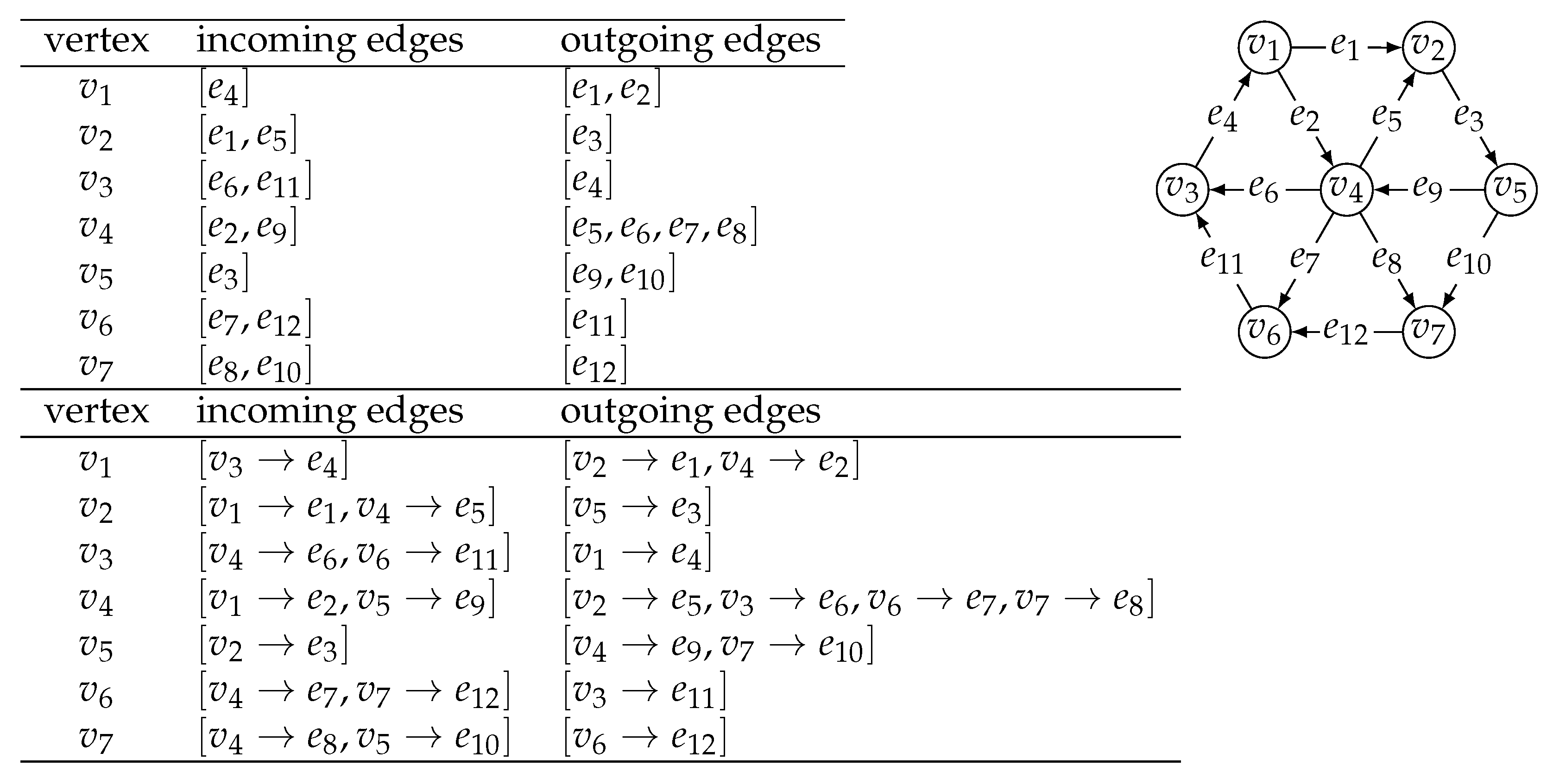
Definition 1. Let be a graph with n vertices and m edges. The adjacency list representation of G consists of a list of n elements (the vertices of the graph), a list of m elements (the edges of the graph), and two lists of n lists of a total of m elements (the edges of the graph). The incoming list corresponding to vertex v contains all edges coming into vertex v, for all vertices . The outgoing list corresponding to vertex v contains all edges going out of vertex v, for all vertices . The source vertex v and the target vertex w are associated with each edge .
The adjacency list representation of a directed graph is illustrated in
Figure 1. The small collection of 11 abstract operations can be implemented using the adjacency list representation to take
time, with the exception of
, which takes
time, and
, which takes
time, as follows:
and are respectively the list of vertices and the list of edges of graph G.
and are respectively the list of edges coming into vertex v and the list of edges going out of vertex v.
is implemented by scanning the list of edges going out of vertex v, or the list of edges coming into vertex w.
and are respectively the source and the target vertex associated with edge e.
is implemented by appending a new vertex v to the list of vertices of graph G, and returning vertex v.
is implemented by appending a new edge e to the list of edges of graph G, setting to v the source vertex associated with edge e, setting to w the target vertex associated with edge e, appending e to the list of edges going out of vertex v and to the list of edges coming into vertex w, and returning edge e.
is implemented by performing for each edge e in the list of edges coming into vertex v and for each edge e in the list of edges going out of vertex v, and then deleting vertex v from the list of vertices of graph G.
is implemented by deleting edge e from the list of edges of graph G, from the list of edges coming into vertex , and from the list of edges going out of vertex .
The adjacency list representation of a graph
with
n vertices and
m edges takes
space, and it allows for implementing graph algorithms such as depth-first search, biconnectivity, acyclicity, planarity testing, topological sorting, and many others to take
time [
6,
7].
In the adjacency list representation of a graph, edges can also be made explicit by replacing the lists of incoming and outgoing edges with dictionaries of source vertices to incoming edges and target vertices to outgoing edges. This allows for a more efficient adjacency test, although adding a logarithmic factor to the cost to all of the operations (when dictionaries are implemented using balanced trees) or turning the worst-case cost for all of the operations into expected cost (when dictionaries are implemented using hashing).
Such a representation was advocated in [
5,
8], and adopted as the default graph representation in the NetworkX package for network analysis in Python [
9]. Essentially, the adjacency map representation of a graph consists of a dictionary
D of vertices to a pair of dictionaries of vertices to edges: a first dictionary
I of source vertices to incoming edges, and a second dictionary
O of target vertices to outgoing edges.
Definition 2. Let be a graph with n vertices and m edges. The adjacency map representation of G consists of a dictionary of n elements (the vertices of the graph) to a pair of dictionaries of m elements (the source and target vertices for the edges of the graph, respectively). The incoming dictionary corresponding to vertex v contains the mappings for all edges coming into vertex v, for all vertices . The outgoing dictionary corresponding to vertex v contains the mappings for all edges going out of vertex v, for all vertices .
The adjacency map representation of a directed graph is also illustrated in
Figure 1. The small collection of 11 abstract operations can also be implemented using the adjacency map representation to take
expected time, with the exception of
, which takes
expected time, as follows:
are the keys in dictionary D.
are the values for all keys v in dictionary D and for all keys w in dictionary .
are the values for all keys u in dictionary .
are the values for all keys w in dictionary .
is true if , where , and false otherwise.
is the source vertex associated with edge e.
is the target vertex associated with edge e.
is implemented by inserting an entry in dictionary D, with the key as a new vertex v and value a pair of empty dictionaries and , and returning vertex v.
is implemented by setting to v the source vertex associated with a new edge e, setting to w the target vertex associated with edge e, inserting an entry in dictionary with key w and value e, inserting an entry in dictionary with key v and value e, and returning edge e.
is implemented by performing for each entry with key u and value e in dictionary and for each entry with key w and value e in dictionary , and then deleting the entry with key v from dictionary D.
is implemented by deleting the entry with key w from dictionary and deleting the entry with key v from dictionary , where and .
Similar to the adjacency list representation, the adjacency map representation of a graph with n vertices and m edges also takes space. In addition to the low space requirement, the main advantage of the adjacency map representation is the support of the adjacency test in expected time, when dictionaries are implemented using hashing.
In this article, we compare the performance of three graph algorithms on a large benchmark dataset of random directed graphs, when implemented with an adjacency-list and an adjacency-map representation, and we show that they run faster on the average with adjacency maps than with adjacency lists.
2. Materials and Methods
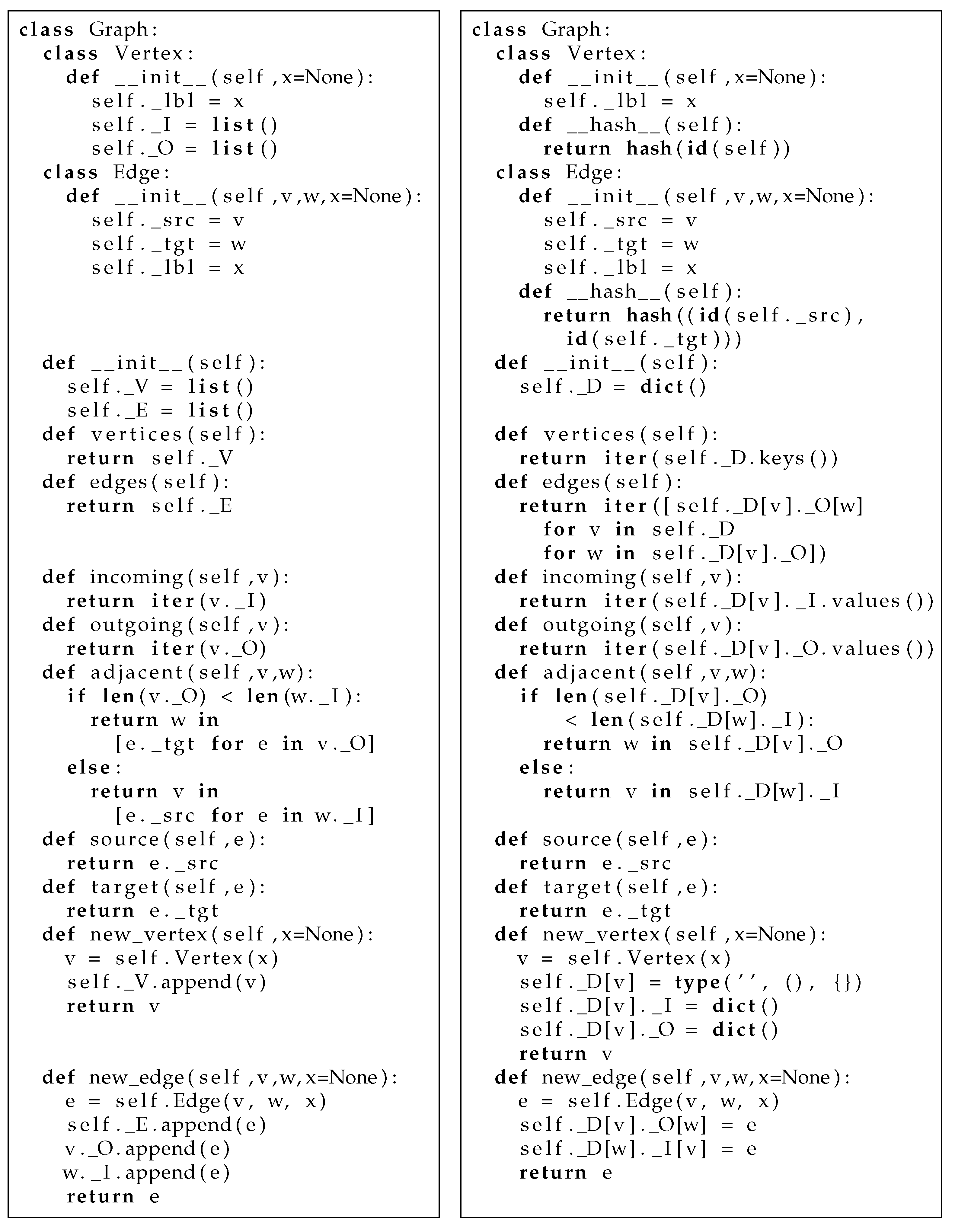
We have implemented 9 of the 11 abstract operations on graphs in Python, namely
for both the adjacency list and the adjacency map representation, and for labeled vertices and edges.
Figure 2 shows the corresponding classes in detail.
For the benchmark dataset, we have used random directed graphs with
vertices and
directed edges. These 86,856 directed graphs were generated using the Erdős–Rényi model, by which all (directed) graphs with
n vertices and
m (directed) edges have the same probability [
10,
11], as implemented in the NetworkX package for network analysis in Python [
9].
In order to compare the performance of the adjacency-list and the adjacency-map representation, we have chosen three graph algorithms:
The universal sink algorithm, adapted from [
1], is shown in Algorithm 2. The first loop, which breaks at the first iteration, is used to set an initial candidate for the universal sink to the first vertex in the order fixed by the representation of the graph (actually, any vertex of the graph would suffice). The second loop is used to discard all but one of the vertices in the graph as candidates for universal sink. The third loop is used to check if the remaining candidate vertex indeed has in-degree equal to the number of vertices of the graph minus one and out-degree zero.
| Algorithm 2 Finding a universal sink in a directed graph with . |
| function universal_sink(G)
|
| for all do |
| break |
| for all do |
| if and then |
| |
| for all do |
| if or ( and not ) then |
| return false |
| return true |
Assuming the adjacency test takes time, the graph construction algorithm, the breadth-first graph traversal algorithm, and the universal sink algorithm all take time, on a graph with n vertices and m directed edges.
3. Results
We have implemented the simple graph construction algorithm and the universal sink algorithm in Python, taken the Python implementation of the breadth-first graph traversal algorithm from ([
5] [Appendix A]), and run the algorithms for graph construction, breadth-first traversal, and universal sink on the 86,856 random directed graphs in the benchmark dataset.
Table 1 shows the average running time of each of the three algorithms with the adjacency-list and the adjacency-map representation, over
= 56, 240, 992, 4032, 16,256, 65,280 random directed graphs with
vertices, respectively, on a computer with a 12-core Intel Xeon processor and 64 GB of memory.
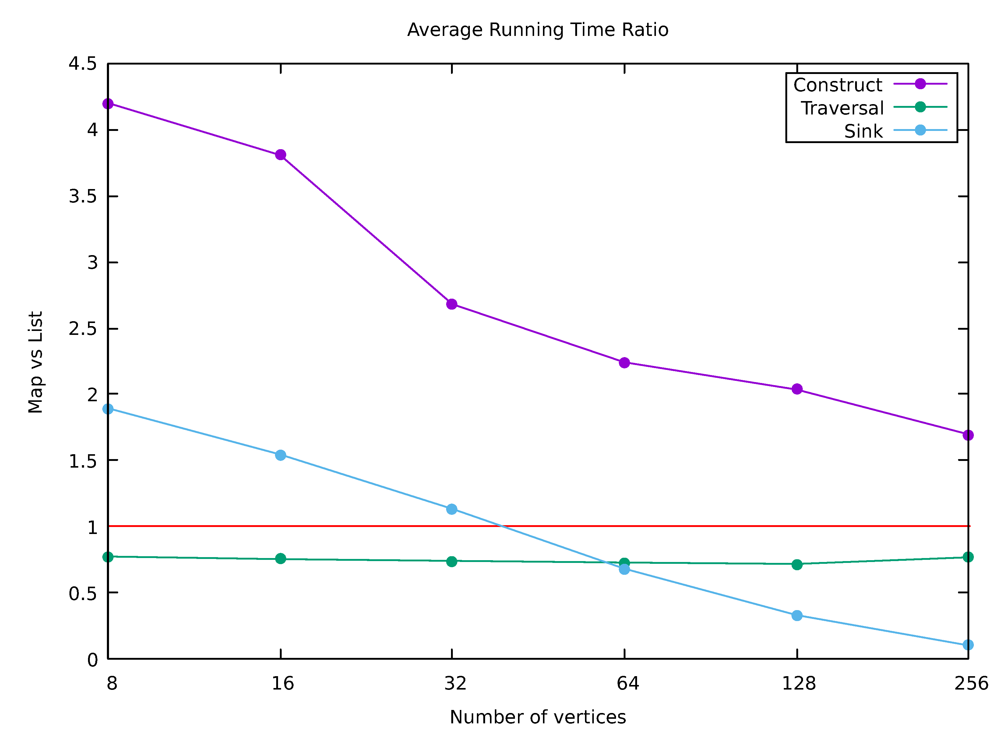
The ratio of these average running times (adjacency maps over adjacency lists) for the three graph algorithms are plotted in
Figure 3. Graph construction is about 4 times slower with adjacency maps for graphs with at most 16 vertices, but only about 2 times slower for graphs with at least 128 vertices. On the other hand, breadth-first graph traversal and the universal sink algorithm run faster with adjacency maps for all graph sizes in the case of graph traversal and for graphs with at least 64 vertices in the case of universal sink on the average.
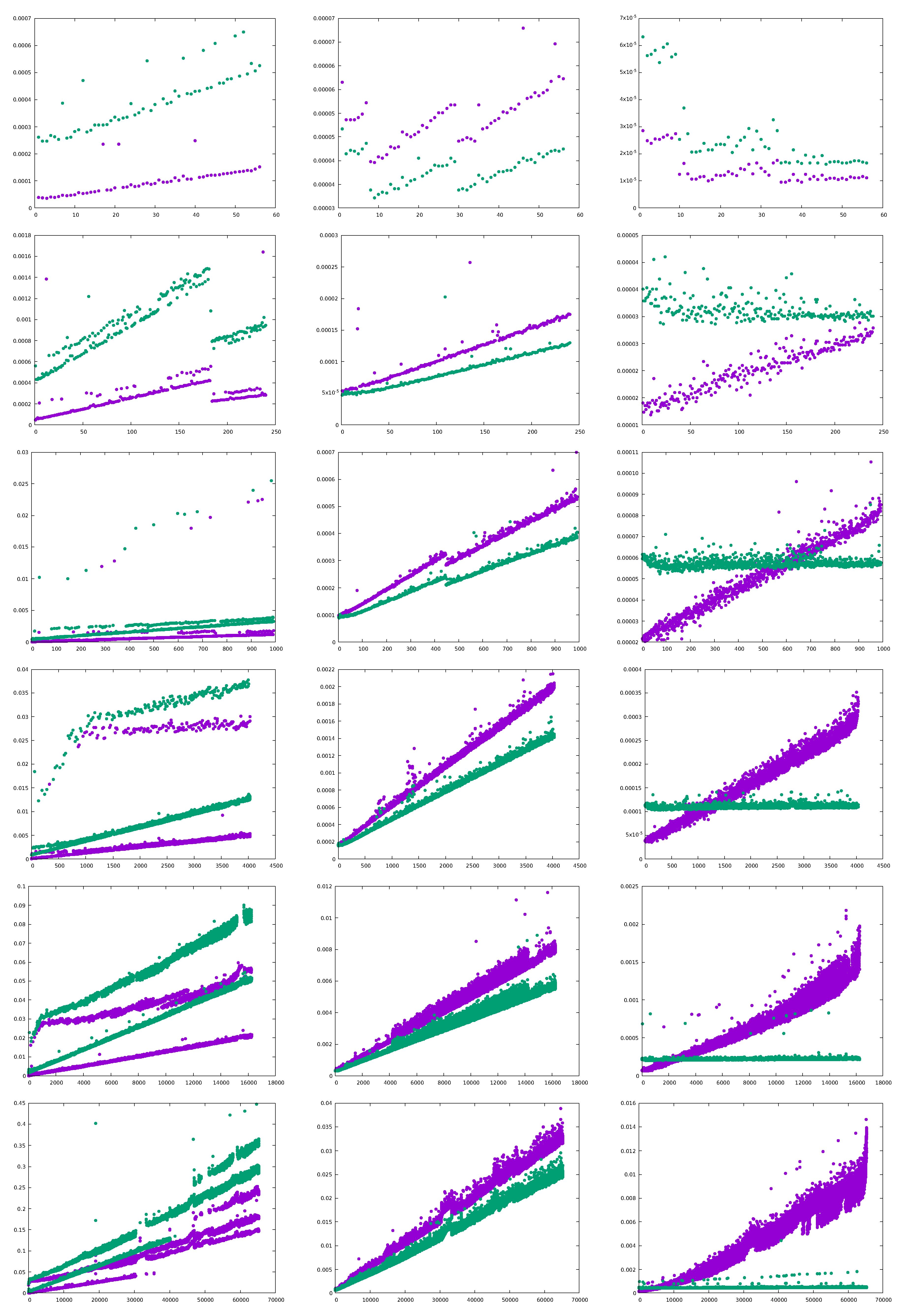
These running times are shown in more detail in
Figure 4, where instead of average running times, individual running times are plotted for each of the random directed graphs in the benchmark dataset. Graph construction is almost always slower with adjacency maps for graphs with 8, 16, or 32 vertices, but it is faster with adjacency maps for 170 of the 4032 graphs with 64 vertices, 2870 of the 16,256 graphs with 128 vertices, and 3599 of the 65,280 graphs with 256 vertices in the benchmark dataset.
Breadth-first graph traversal is almost always faster with adjacency maps: for all the 56 graphs with 8 vertices, 239 of the 240 graphs with 16 vertices, 989 of the 992 graphs with 32 vertices, 4022 of the 4032 graphs with 64 vertices, 16,247 of the 16,256 graphs with 128 vertices, and 65,266 of the 65,280 graphs with 256 vertices in the benchmark dataset. The universal sink algorithm is always slower with adjacency maps for graphs with 8 or 16 vertices, but it is faster with adjacency maps for 394 of the 992 graphs with 32 vertices, 2828 of the 4032 graphs with 64 vertices, 13,839 of the 16,256 graphs with 128 vertices, and 60,582 of the 65,280 of the graphs with 256 vertices in the benchmark dataset.
4. Discussion
We have implemented three graph algorithms (graph construction, breadth-first graph traversal, and universal sink) using a small collection of abstract operations, with both the adjacency-list and the adjacency-map representation, and run them upon a benchmark dataset of random directed graphs with vertices and a number of directed edges ranging from to the maximum possible number of directed edges. The abstract operations take worst-case time with the adjacency-list representation and expected time with the adjacency-map representation, with the only exception of the adjacency test, which takes worst-case linear time in the degree of the vertices with the adjacency-list representation. With the adjacency-map representation, the abstract operations used in the algorithm for graph construction require dictionary lookup and update, and the abstract operations used in the algorithms for breadth-first graph traversal and for finding a universal sink require dictionary lookup, iteration over dictionary keys, and iteration over dictionary values.
The experimental results show that graph construction is slower (by a small constant factor) with adjacency maps than with adjacency lists. This can be explained by the amortized running time of the underlying update operations on dynamic lists and dictionaries. Adding a new vertex to a graph involves one list-append operation with adjacency lists, and one insertion in a dictionary and the creation of two new dictionaries with adjacency maps, while adding a new edge to a graph involves three list-append operations with adjacency lists and two insertions in a dictionary with adjacency maps. Nevertheless, extending the adjacency-map representation with an operation to build a graph from a list of edges, instead of adding vertices and edges one-by-one to an initially empty graph, might result in a faster graph construction algorithm.
Experimental results also show that graph algorithms that do not test adjacencies (breadth-first graph traversal) run faster (by a small constant factor) with adjacency maps than with adjacency lists, and graph algorithms that test adjacencies (universal sink) run much faster (by one or two orders of magnitude) with adjacency maps than with adjacency lists. These results further reinforce the choice of the adjacency-map representation over the adjacency-list representation in recent textbooks [
5,
8] and software libraries [
9].
While the experimental results were obtained with a Python implementation of the algorithms and graph data structures, adjacency maps can be easily implemented in any modern programming language, as they only need dictionaries as the underlying data structures. However, it is possible that the differences in running time between adjacency lists and adjacency maps become smaller with compiled programming languages once the overhead of compiling the source code into bytecode by the Python interpreter is removed. The influence of the programming language in the efficiency of the adjacency-map representation is an open line of future research.


