Finding Hamiltonian and Longest (s,t)-Paths of C-Shaped Supergrid Graphs in Linear Time

Abstract

A graph is called Hamiltonian connected if it contains a Hamiltonian path between any two distinct vertices. In the past, we proved the Hamiltonian path and cycle problems for general supergrid graphs to be NP-complete. However, they are still open for solid supergrid graphs. In this paper, first we will verify the Hamiltonian cycle property of C-shaped supergrid graphs, which are a special case of solid supergrid graphs. Next, we show that C-shaped supergrid graphs are Hamiltonian connected except in a few conditions. For these excluding conditions of Hamiltonian connectivity, we compute their longest paths. Then, we design a linear-time algorithm to solve the longest path problem in these graphs. The Hamiltonian connectivity of C-shaped supergrid graphs can be applied to compute the optimal stitching trace of computer embroidery machines, and construct the minimum printing trace of 3D printers with a C-like component being printed.

1. Introduction

A Hamiltonian path (cycle) in a graph is a spanning path (cycle) of the graph. The Hamiltonian path (cycle) problem involves deciding whether or not a graph contains a Hamiltonian path (cycle). A graph is called Hamiltonian if it contains a Hamiltonian cycle. A graph G is said to be Hamiltonian connected if for each pair of distinct vertices u and v of G, there is a Hamiltonian path between u and v in G. It is well known that the Hamiltonian path and cycle problems are NP-complete for general graphs [1]. In [2], Harary outlined the important motivations and applications for Hamiltonian path problem. In addition, the Hamiltonian problems have been much studied and have numerous applications in different areas, including establishing transport routes, production launching, the on-line optimization of flexible manufacturing systems [3], computing the perceptual boundaries of dot patterns [4], pattern recognition [5,6,7], hypercube properties [8], molecular and physical sciences [9,10], biology science [11], etc. It is worth mentioning that Twarock et al. [11] applied the Hamiltonian path to the analysis of viral genomes, and Balasubramanian [9,10] pointed out that in molecular and physical sciences, the Hamiltonian path problem is related to random walks, enumeration of self-returning walks and ring perception algorithms, and peripherals of fullerenes. The longest path problem, which finds a simple path with the maximum number of vertices in a graph, is one of the most important problems in graph theory. The Hamiltonian path problem is clearly a special case of the longest path problem. Despite the many applications of the problem, it is still open for some classes of graphs, including solid supergrid graphs and supergrid graphs with some holes [12]. There are few classes of graphs in which the longest path problem is polynomial-time solvable [13,14,15]. Because the time complexity of the longest path problem on solid supergrid graphs is still open, it is interesting to study this problem for the subcalsses of solid supergrid graphs. In this paper, we focus on C-shaped supergrid graphs, which form a subclass of solid supergrid graphs. We will give the necessary and sufficient conditions for the Hamiltonicity and Hamiltonian connectivity of C-shaped supergrid graphs. We also present a linear-time algorithm for finding a longest path between any two distinct vertices in a C-shaped supergrid graph.

The two-dimensional integer grid graph $G^{\infty }$ is an infinite graph whose vertex set consists of all points of the Euclidean plane with integer coordinates and in which two vertices are adjacent if the (Euclidean) distance between them is 1. The two-dimensional supergrid graph$S^{\infty }$ is an infinite graph obtained from $G^{\infty }$ by adding all edges on the lines traced from up-left to down-right and from up-right to down-left. A graph is a grid graph if it is a finite induced subgraph of $G^{\infty }$. A supergrid graph is a finite vertex-induced subgraph of $S^{\infty }$. Supergrid graphs came from our industry-university cooperative research project, and can be applied to compute the stitching trace of computerized sewing machines [16]. A solid supergrid graph is a supergrid graph without any hole, and a rectangular supergrid graph is a solid supergrid graph bounded by a axis-parallel rectangle. A L-shaped or C-shaped supergrid graph is a supergrid graph obtained from a rectangular supergrid graph by removing a rectangular supergrid subgraph from it to form a L-like or C-like shape.

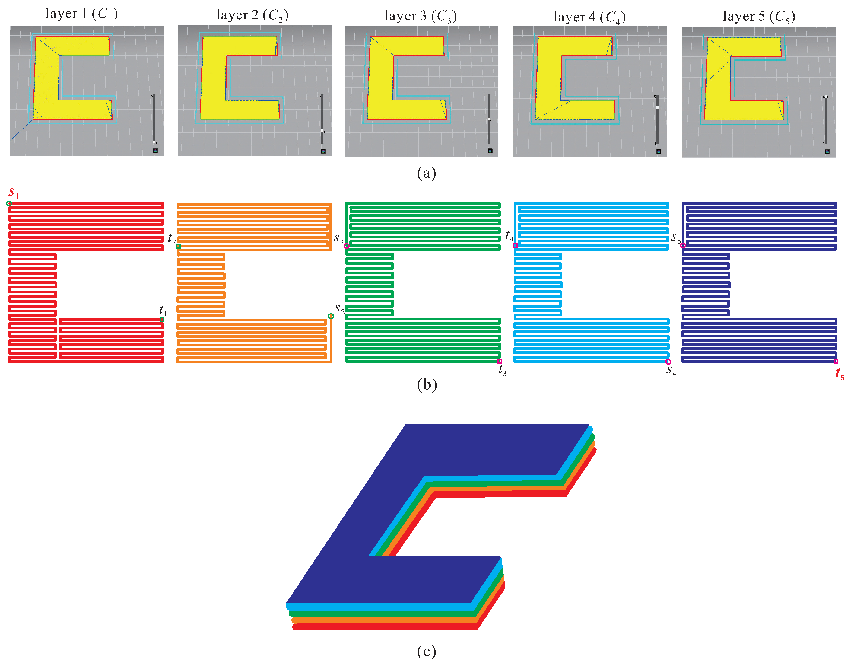
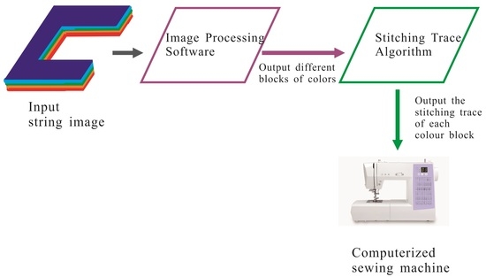
The Hamiltonian connectivity and longest path of shaped supergrid graphs can be applied for computing the optimal stitching trace of computer embroidery machines [12,16,17]. For example, consider that a string of letters will be sewed into an object such that the number of crossed paths is minimum. The Hamiltonian connectivity and longest path of these shaped letters play an important role in deciding these sewing traces. In addition, they can be also applied to construct the minimum printing trace of 3D printers. 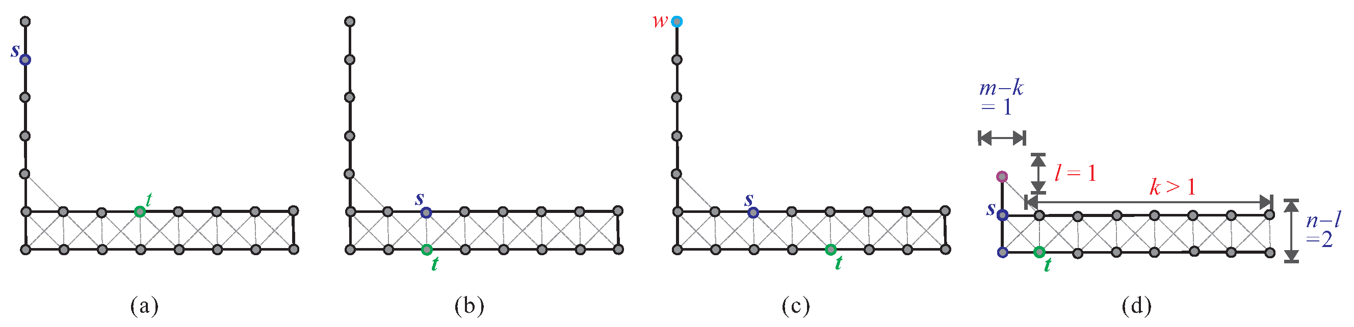For example, consider a 3D printer with a C-like object being printed. The software produces a series of thin layers, designs a path for each layer, combines these paths of produced layers, and transmits the above paths to 3D printer. Because 3D printing is performed layer-by-layer (see Figure 1a), each layer can be considered as a C-shaped supergrid graph. Suppose that there are k layers under the above 3D printing. If the Hamiltonian connectivity of C-shaped supergrid graphs holds true, then we can find a Hamiltonian path, starting from $s_i$ and ending at $t_i$, of a C-shaped supergrid graph $C_i$, where $C_i$, $1⩽i⩽k$, represents a layer under 3D printing. Thus, we can design an optimal trace for the above 3D printing, where $t_i$ is adjacent to $s_{i+1}$ for $1⩽i⩽k-1$. In this application, we restrict the 3D printer nozzle to be located at integer coordinates. For example, Figure 1a shows five layers $C_1$–$C_5$ of a 3D printing for a C-type object, Figure 1b depicts the Hamiltonian paths of $C_i$ for $1⩽i⩽5$, and the result of this 3D printing is shown in Figure 1c.

Some related works in the literature are summarized as follows. Recently, Hamiltonian path (cycle) and Hamiltonian connected problems in grid and supergrid graphs have received much attention. In [18], Itai et al. proved that the Hamiltonian path problem on grid graphs is NP-complete. They also gave necessary and sufficient conditions for a rectangular grid graph having a Hamiltonian path between two given vertices. Note that rectangular grid graphs are not Hamiltonian connected. Zamfirescu et al. [19] gave sufficient conditions for a grid graph having a Hamiltonian cycle, and proved that all grid graphs of positive width have Hamiltonian line graphs. Later, Chen et al. [20] improved the Hamiltonian path algorithm of [18] on rectangular grid graphs and presented a parallel algorithm for the Hamiltonian path problem with two given endpoints in rectangular grid graphs. In addition, there is a polynomial-time algorithm for finding Hamiltonian cycles in solid grid graphs [21]. However, the Hamiltonian problems are still open for solid supergrid graphs. In [22], Salman introduced alphabet grid graphs and determined classes of alphabet grid graphs which contain Hamiltonian cycles. Supergrid graphs first appeared in [16], and the authors proved that the Hamiltonian cycle and path problems on general supergrid graphs are NP-complete, and every rectangular supergrid graph always contains a Hamiltonian cycle. Recently, the Hamiltonian connectivity of L-shaped supergrid graphs has been verified in [17]. Note that C-shaped supergrid graphs contain L-shaped supergrid graphs as their subgraphs. Thus, the results of L-shaped supergrid graphs can not be directly applied to C-shaped supergrid graphs. However, the results in [17] will be used in our method. In this paper, we will consider the Hamiltonian, Hamiltonian connectivity, and longest path of C-shaped supergrid graphs.

The rest of the paper is organized as follows. In Section 2, some notations, observations, known results, and one special Hamiltonian connected property of a special rectangular supergrid graph are given. In Section 3, we give the necessary and sufficient conditions for the Hamiltonian and the Hamiltonian connected C-shaped supergrid graphs. This section shows that C-shaped supergrid graphs are always Hamiltonian and Hamiltonian connected except for a few conditions. In Section 4, we present a linear-time algorithm to compute the longest path between any two distinct vertices in a C-shaped supergrid graph. Finally, a conclusion is given in Section 5.

2. Terminologies and Background Results

In this section, we will introduce some terminologies and symbols. Some observations and previously established results for the Hamiltonicity and Hamiltonian connectivity of rectangular and L-shaped supergrid graphs are also given. In addition, we also prove some Hamiltonian connectivity property of a special class of rectangular supergrid graphs that will be used in proving our result.

Suppose that G is a graph with vertex set $V\left(G\right)$ and edge set $E\left(G\right)$. Let $S\subseteq V\left(G\right)$, and let $u,v\in V\left(G\right)$. We write $G\left[S\right]$ for the subgraph of G induced by S, and $G-S$ for the subgraph $G\left[V\right(G)-S]$. In general, we write $G-v$ instead of $G-\left\{v\right\}$. The notation $u\sim v$ (resp., $u\nsim v$) means that vertices u and v are adjacent (resp., non-adjacent). A vertex wadjoins edge $(u,v)$ if $w\sim u$ and $w\sim v$. For two edges $e_1=(u_1,v_1)$ and $e_2=(u_2,v_2)$, if $u_1\sim u_2$ and $v_1\sim v_2$ then we say that $e_1$ and $e_2$ are parallel, denoted this by $e_1\approx e_2$. A neighbor of vertex v is any vertex adjacent to v. We denote by $N_G\left(v\right)$ the set of neighbors of v in G, and let $N_G\left[v\right]=N_G\left(v\right)\cup \left\{v\right\}$. The degree of vertex v in G, denoted by $deg\left(v\right)$, is the number of vertices adjacent to v. A path P of length $\left|P\right|$ in G, denoted by $v_1\to v_2\to \cdots \to v_{\left|P\right|-1}\to v_{\left|P\right|}$, is a sequence $(v_1,v_2,\cdots ,v_{\left|P\right|-1},v_{\left|P\right|})$ of vertices such that $(v_i,v_{i+1})\in E\left(G\right)$ for $1⩽i<\left|P\right|$, and all vertices except $v_1,v_{\left|P\right|}$ in it are distinct. The first and last vertices visited by P are denoted by $start\left(P\right)$ and $end\left(P\right)$, respectively. We will use $v_i\in P$ to denote “P visits vertex $v_i$” and use $(v_i,v_{i+1})\in P$ to denote “P visits edge $(v_i,v_{i+1})$”. A path from $v_1$ to $v_k$ is denoted by $(v_1,v_k)$-path. In addition, we use P to refer to the set of vertices visited by path P if it is understood without ambiguity. A cycle is a path C with $\left|V\right(C\left)\right|⩾3$ and $start\left(C\right)=end\left(C\right)$. Two paths (or cycles) $P_1$ and $P_2$ of graph G are vertex-disjoint if $V\left(P_1\right)\cap V\left(P_2\right)=\varnothing$. If $end\left(P_1\right)\sim start\left(P_2\right)$, then two vertex-disjoint paths $P_1$ and $P_2$ can be concatenated into a path, denoted by $P_1\Rightarrow P_2$.

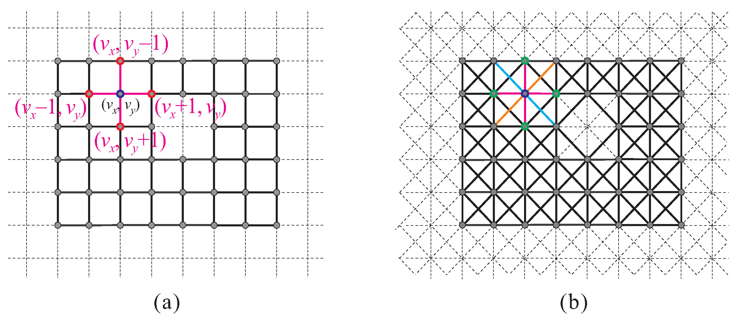
For a node (vertex) v in the plane with integer coordinates, let $v_x$ and $v_y$ represent the x and ycoordinates of node v, respectively, denoted by $v=(v_x,v_y)$. A grid graph is a finite vertex-induced subgraph of $G^{\infty }$. Figure 2a shows a grid graph, and it is clear that the maximum degree of all vertices is four. A supergrid graph is a finite vertex-induced subgraph of $S^{\infty }$. Figure 2b depicts a supergrid graph, it is clear that the maximum degree of all vertices is eight. Thus, supergrid graphs contain grid graphs as subgraphs. Notice that grid graphs are not a subclass of supergrid graphs, and the converse is also true. Obviously, all grid graphs are bipartite [18] but supergrid graphs are not bipartite.

A rectangular supergrid graph, denoted by $R(m,n)$, is a supergrid graph whose vertex set is $V\left(R(m,n)\right)=\{v=(v_x,v_y)|1⩽v_x⩽m$ and $1⩽v_y⩽n\}$. That is, $R(m,n)$ contains m columns and n rows of vertices in $S^{\infty }$ and its shape is a rectangle. The size of $R(m,n)$ is defined to be $mn$, and $R(m,n)$ is called n-rectangle. The vertex v is called the upper-left (resp., upper-right, down-left, down-right) corner of $R(m,n)$ if for any vertex $w=(w_x,w_y)\in R(m,n)$, $w_x⩾v_x$ and $w_y⩾v_y$ (resp., $w_x⩽v_x$ and $w_y⩾v_y$, $w_x⩾v_x$ and $w_y⩽v_y$, $w_x⩽v_x$ and $w_y⩽v_y$). 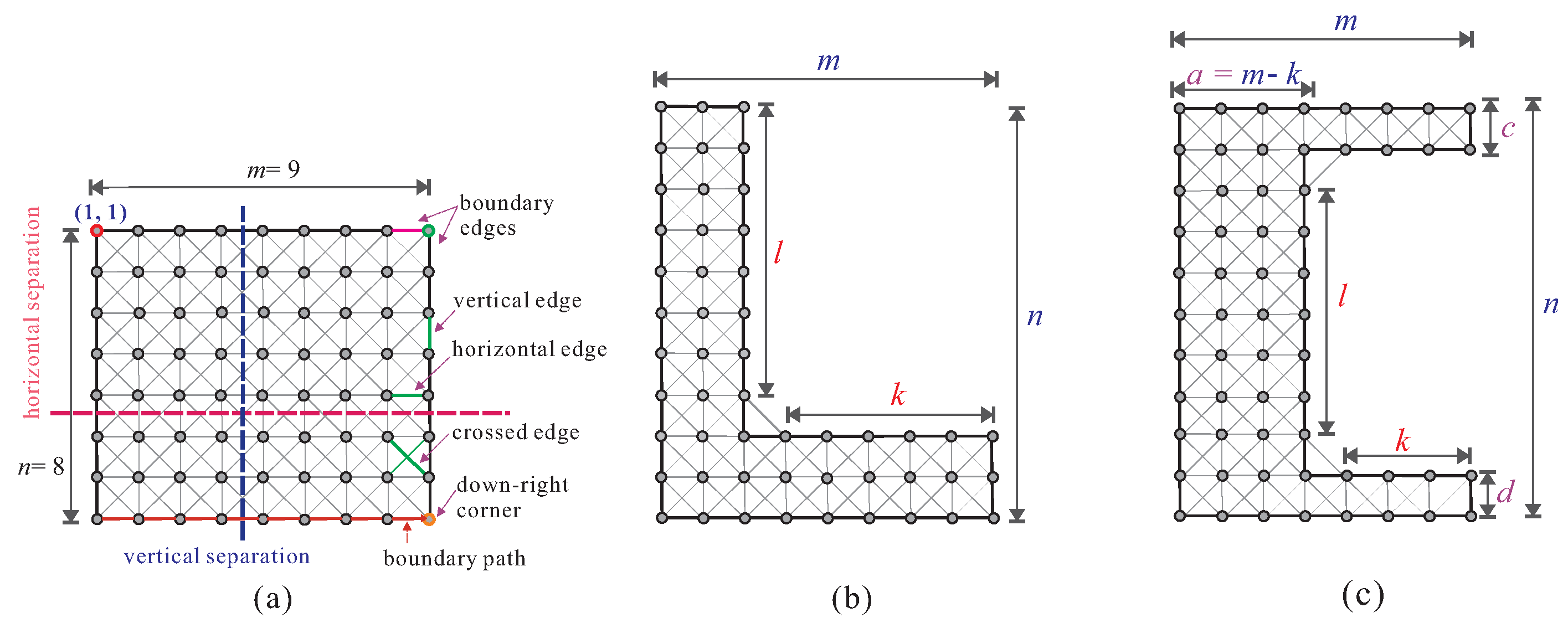The edge $(u,v)$ is said to be horizontal (resp., vertical) if $u_y=v_y$ (resp., $u_x=v_x$), and is called crossed if it is neither a horizontal nor a vertical edge. There are four boundaries in a rectangular supergrid graph $R(m,n)$ with $m,n⩾2$. The edge in the boundary of $R(m,n)$ is called boundary edge. A path is called boundary of $R(m,n)$ if it visits all vertices and edges of the same boundary in $R(m,n)$ and its length equals to the number of vertices in the visited boundary. For example, Figure 3a shows a rectangular supergrid graph $R(9,8)$ which is called 8-rectangle and contains $2\times (8+7)=30$ boundary edges. Figure 3a also indicates the types of edges and corners. In the figures we will assume that $(1,1)$ are coordinates of the upper-left corner in $R(m,n)$, except when we explicitly change this assumption.

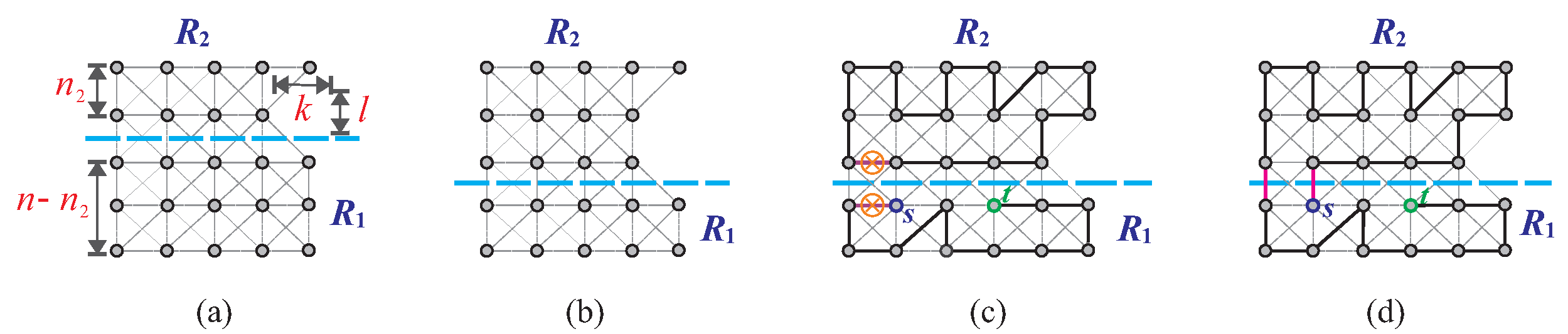
A L-shaped supergrid graph, denoted by $L(m,n;k,l)$, is a supergrid graph obtained from a rectangular supergrid graph $R(m,n)$ by cutting its subgraph $R(k,l)$ from the upper-right corner, where $m,n>1$ and $k,l⩾1$. A C-shaped supergrid graph $C(m,n;k,l;c,d)$ is a supergrid graph obtained from a rectangular supergrid graph $R(m,n)$ by removing its subgraph $R(k,l)$ from its node coordinated as $(m,c+1)$ while $R(m,n)$ and $R(k,l)$ have exactly one border side in common, where $m⩾2$, $n⩾3$, $k,l⩾1$, $c⩾1$, $d=n-l-c⩾1$, and $a=m-k⩾1$. The structures of $L(m,n;k,l)$ and $C(m,n;k,l;c,d)$ are explained in Figure 3b,c, respectively.

In our method, we need to partition a rectangular or C-shaped supergrid graph into $\eta$ disjoint parts, where $\eta ⩾2$. The partition is defined as follows.

Definition 1.

Assume that $\widehat{G}$ is a rectangular supergrid graph $R(m,n)$ or a C-shaped supergrid graph $C(m,n;k,l;c,d)$. A separation operation on $\widehat{G}$ is a partition of $\widehat{G}$ into η vertex-disjoint rectangular or L-shaped supergrid subgraphs ${\widehat{G}}_1$, ${\widehat{G}}_2$, ⋯, ${\widehat{G}}_{\eta }$, i.e., $V\left(\widehat{G}\right)=V\left({\widehat{G}}_1\right)\cup V\left({\widehat{G}}_2\right)\cup \cdots \cup V\left({\widehat{G}}_{\eta }\right)$ and $V\left({\widehat{G}}_i\right)\cap V\left({\widehat{G}}_j\right)=\varnothing$ for $i\ne j$ and $1⩽i,j⩽\eta$, where $\eta ⩾2$. A separation is called horizontal if it consists of a set of vertical edges, and is called vertical if it contains a set of horizontal edges. Note that horizontal or vertical separation may be empty in our partition for the presentation of clarity. For example, Figure 3a indicates a horizontal (resp., vertical) separation of $R(9,8)$ which partitions it into $R(9,3)$ and $R(9,5)$ (resp., $R(4,8)$ and $R(5,8)$).

Let $R(m,n)$ be a rectangular supergrid graph with $m⩾n⩾2$, $\mathcal{C}$ be a cycle of $R(m,n)$, and let H be a boundary of $R(m,n)$. The restriction of $\mathcal{C}$ to H is denoted by ${\mathcal{C}}_{|H}$. If $|{\mathcal{C}}_{|H}|=1$, i.e., ${\mathcal{C}}_{|H}$ is a boundary path on H, then ${\mathcal{C}}_{|H}$ is called flat face on H. If $|{\mathcal{C}}_{|H}|>1$ and ${\mathcal{C}}_{|H}$ contains at least one boundary edge of H, then ${\mathcal{C}}_{|H}$ is called concave face on H. 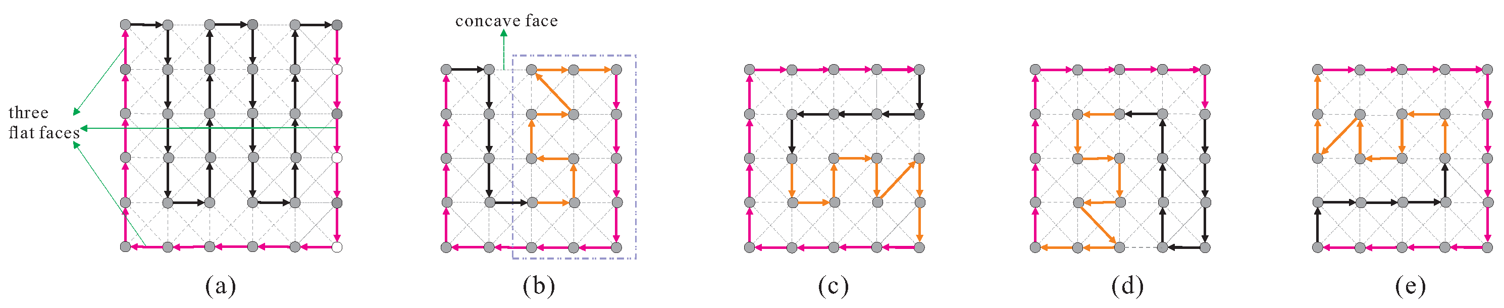A Hamiltonian cycle of $R(m,3)$ is called canonical if it contains three flat faces on two shorter boundaries and one longer boundary, and it contains one concave face on the other boundary, where the shorter boundary consists of three vertices. A Hamiltonian cycle of $R(m,n)$ with $n=2$ or $n⩾4$ is said to be canonical if it contains three flat faces on three boundaries, and it contains one concave face on the other boundary. The following lemma states the result in [16] concerning the Hamiltonicity of rectangular supergrid graphs.

Lemma 1

(See [16]). Assume that $R(m,n)$ is a rectangular supergrid graph with $m⩾n⩾2$. Then, the following statements hold true:

(1)

$R(m,3)$ contains a canonical Hamiltonian cycle;

(2)

$R(m,n)$ with $n=2$ or $n⩾4$ contains four canonical Hamiltonian cycles with concave faces being on different boundaries.

Figure 4 shows canonical Hamiltonian cycles for rectangular supergrid graphs found in Lemma 1. Each Hamiltonian cycle constructed by this lemma contains all the boundary edges on any three sides of the rectangular supergrid graph. This shows that for any rectangular supergrid graph $R(m,n)$ with $m⩾n⩾4$, we can construct four canonical Hamiltonian cycles such that their concave faces are placed on different boundaries. For instance, the four distinct canonical Hamiltonian cycles of $R(5,5)$ are shown in Figure 4b–e.

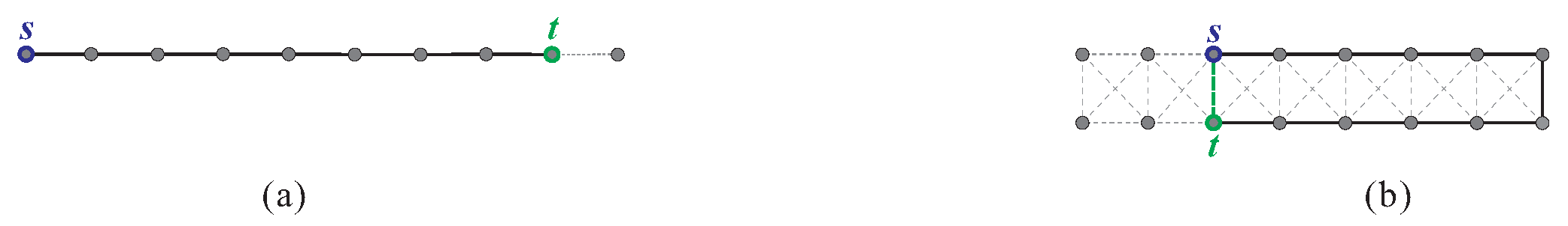
Let $(G,s,t)$ denote supergrid graph G with two specified distinct vertices s and t. Without loss of generality, we will assume that $s_x⩽t_x$ in the rest of the paper. We denote a Hamiltonian path between s and t in G by $HP(G,s,t)$. We say that $HP(G,s,t)$ does exist if there is a Hamiltonian $(s,t)$-path in G. From Lemma 1, $HP\left(R\right(m,n),s,t)$ does exist if $m,n⩾2$ and $(s,t)$ is an edge in the constructed Hamiltonian cycle of $R(m,n)$.

Definition 2.

Assume that G is a connected supergrid graph and $V_1$ is a subset of the vertex set $V\left(G\right)$. $V_1$ is called a vertex cut if $G-V_1$ is disconnected. A vertex $v\in V\left(G\right)$ is said to be a cut vertex if $G-\left\{v\right\}$ is disconnected.

In [12], the authors showed that $HP\left(R\right(m,n),s,t)$ does not exist if the following condition hold:

$\left(\mathrm{F}1\right)$

s or t is a cut vertex, or $\{s,t\}$ is a vertex cut (see Figure 5).

Assume G is any supergrid graph. The following lemma shows that $HP(G,s,t)$ does not exist if $(G,s,t)$ satisfies condition (F1), and can be verified by the same arguments in [23].

Lemma 2

(See [23]). Assume that G is a supergrid graph with two vertices s and t. If $(G,s,t)$ satisfies condition $\left(\mathrm{F}1\right)$, then $HP(G,s,t)$ does not exist.

The Hamiltonian $(s,t)$-path of $R(m,n)$ constructed in [12] satisfies that it contains at least one boundary edge of each boundary, and is called canonical.

Lemma 3

(See [12]). Assume $R(m,n)$ is a rectangular supergrid graph and $s,t\in V\left(R\right(m,n\left)\right)$. If $\left(R\right(m,n),s,t)$ does not satisfy condition $\left(\mathrm{F}1\right)$, then there exists a canonical Hamiltonian $(s,t)$-path of $R(m,n)$.

Lemma 4

(See [17]). Assume $R(m,n)$ is a rectangular supergrid graph with $m⩾3$ and $n⩾2$, and s and t are its two distinct vertices. Let $w=(1,1)$, $z=(2,1)$, and $f=(3,1)$. If $\left(R\right(m,n),s,t)$ does not satisfy condition $\left(\mathrm{F}1\right)$, then there exists a canonical Hamiltonian $(s,t)$-path P of $R(m,n)$ such that $(z,f)\in P$ if $\left(R\right(m,n),s,t)$ does satisfy condition $\left(\mathrm{F}2\right)$; and $(w,z)\in P$ otherwise, where condition $\left(\mathrm{F}2\right)$ is defined as follows:

$\left(\mathrm{F}2\right)$

$n=2$ and $\{s,t\}\in \left\{\right\{w,z\},\{(1,1),(2,2)\},\{(2,1),(1,2)\left\}\right\}$, or $n⩾3$ and $\{s,t\}=\{w,z\}$.

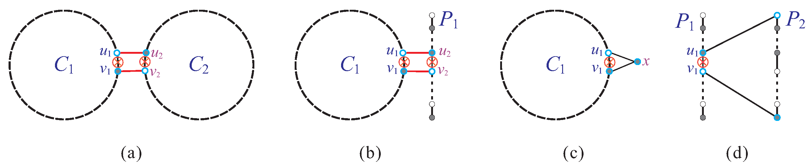
We then give some observations on the relations among cycle, path, and vertex. These propositions will be used in proving our results and are given in [12].

Proposition 1

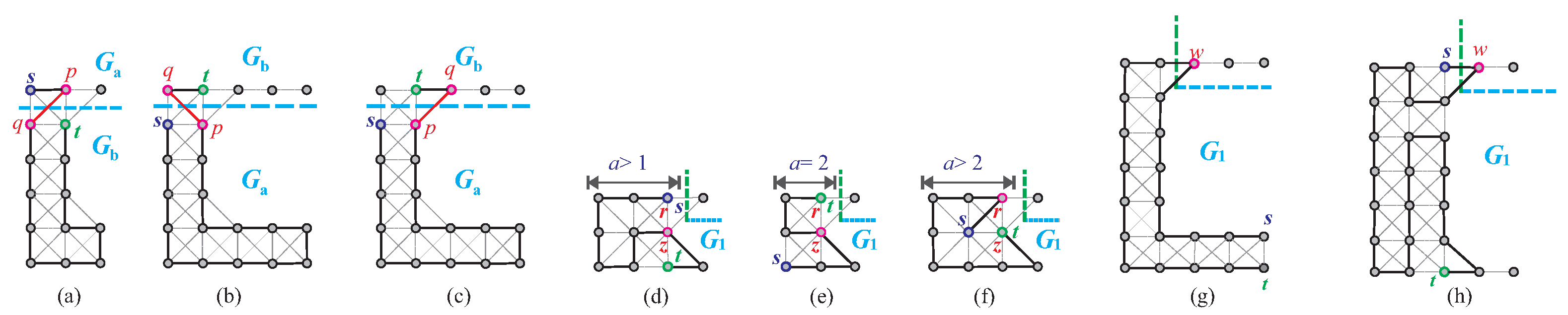
(See [12]). Let G be a graph. Assume $C_1$ and $C_2$ are two vertex-disjoint cycles of G, $P_1$ and $P_2$ are two vertex-disjoint paths of G, $C_1$ and $P_1$ are a cycle and a path, respectively, of G with $V\left(C_1\right)\cap V\left(P_1\right)=\varnothing$, and assume x is a vertex in $G-V\left(C_1\right)$ or $G-V\left(P_1\right)$. Then, the following statements hold true:

(1)

If there exist two edges $e_1\in C_1$ and $e_2\in C_2$ such that $e_1\approx e_2$, then $C_1$ and $C_2$ can be combined into a cycle of G (see Figure 6a).

(2)

If there exist two edges $e_1\in C_1$ and $e_2\in P_1$ such that $e_1\approx e_2$, then $C_1$ and $P_1$ can be combined into a path of G (see Figure 6b).

(3)

If vertex x adjoins one edge $(u_1,v_1)$ of $C_1$ (resp., $P_1$), then $C_1$ (resp., $P_1$) and x can be merged into a cycle (resp., path) of G (see Figure 6c).

(4)

If there exists one edge $(u_1,v_1)\in P_1$ such that $u_1\sim start\left(P_2\right)$ and $v_1\sim end\left(P_2\right)$, then $P_1$ and $P_2$ can be combined into a path of G (see Figure 6d).

Next, we will discover one Hamiltonian connected property of 3-rectangle $R(m,3)$ with $m⩾3$ that will be used in to prove our result. Let $z_1=(m,1)$, $z_2=(m,2)$, and $z_3=(m,3)$ be three vertices of $R(m,3)$. Assume that $\tilde{R}=R(m,3)-\{z_1,z_2,z_3\}$ and edges $e_{12}=(z_1,z_2)$, $e_{23}=(z_2,z_3)$. Assume that $s,t\in \tilde{R}$. We will prove that there exists a Hamiltonian $(s,t)$-path P of $R(m,3)$ such that $e_{12},e_{23}\in P$. Before giving this property, we first give one result in [12] for 3-rectangle as follows.

Lemma 5

(See [12]). Assume $R(m,3)$ is a 3-rectangle with $m⩾3$ and $s,t$ being its two distinct vertices. Then, $R(m,3)$ contains a canonical Hamiltonian $(s,t)$-path which contains at least one boundary edge of each boundary in $R(m,3)$.

By using the above lemma, we will prove the following lemma.

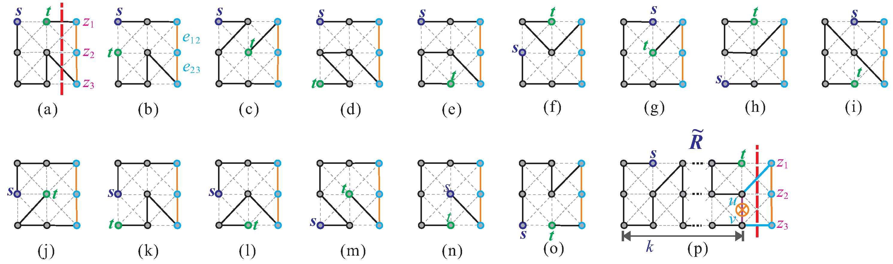
Lemma 6.

Assume $R(m,3)$ is a 3-rectangle with $m⩾3$ and $s,t$ being its two distinct vertices. Let $z_1=(m,1)$, $z_2=(m,2)$, and $z_3=(m,3)$, which are the three vertices of $R(m,3)$, and let edges $e_{12}=(z_1,z_2)$, $e_{23}=(z_2,z_3)$. If $\{s,t\}\cap \{z_1,z_2,z_3\}=\varnothing$, then there exists a Hamiltonian $(s,t)$-path of $R(m,3)$ containing $e_{12}$ and $e_{23}$.

Proof. 

We will prove this lemma by induction on m. Let $\tilde{R}=R(m,3)-\{z_1,z_2,z_3\}$. Then, $\tilde{R}=R(m-1,3)$, where $m-1⩾2$. Initially, let $m=3$. Then, $\tilde{R}=R(2,3)$ and $s,t\in \tilde{R}$. By considering every case, we can construct the desired Hamiltonian $(s,t)$-path of $R(3,3)$, as shown in Figure 7a–o. Assume that the lemma holds true when $m=k⩾3$. Consider that $m=k+1$. Then, $\tilde{R}=R(k,3)$ is a subgraph of $R(k+1,3)$, where $z_1=(k+1,1)$, $z_2=(k+1,2)$, $z_3=(k+1,3)$, and $s,t\in \tilde{R}=R(k,3)$. Let $\widehat{P}=z_1\to z_2\to z_3$. By Lemma 5, $\tilde{R}$ contains a Hamiltonian $(s,t)$-path $\tilde{P}$ such that it contains an edge $\tilde{e}=(u,v)$ locating to face $R(k+1,3)-\tilde{R}$. Then, $start\left(\widehat{P}\right)\sim u$ and $end\left(\widehat{P}\right)\sim v$. By Statement (4) of Proposition 1, $\tilde{P}$ and $\widehat{P}$ can be combined into a Hamiltonian $(s,t)$-path of $R(k+1,3)$. The construction of such a Hamiltonian path is depicted in Figure 7p. Thus, the lemma holds when $m=k+1$. By induction, the lemma holds true.    □

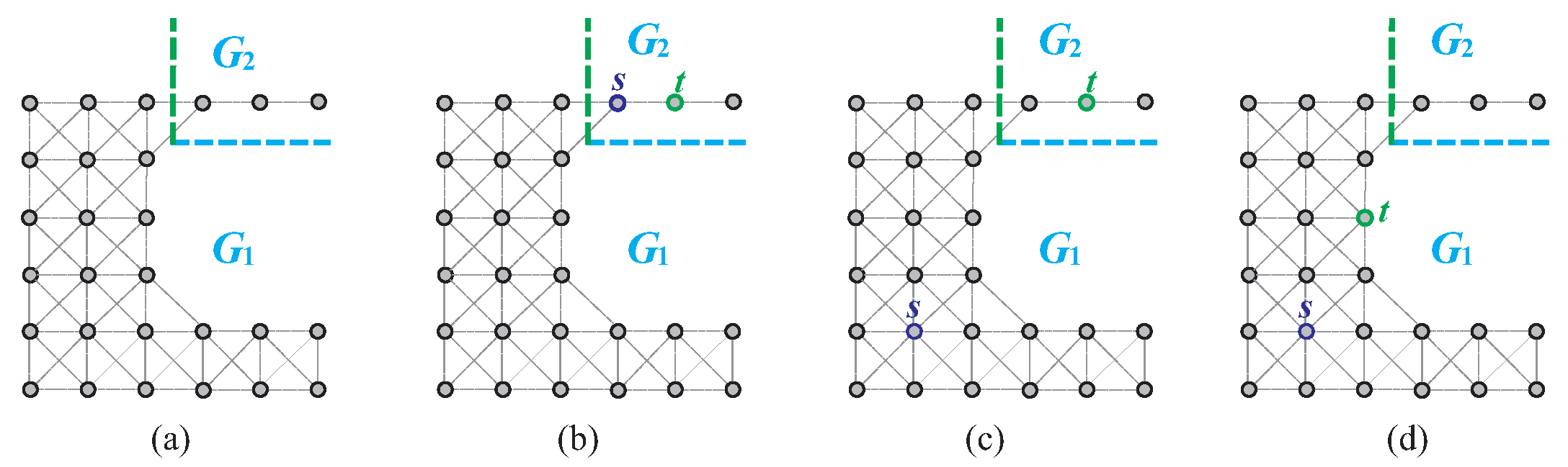
In addition to condition (F1) (see Figure 8a,b), in [17], we showed that $HP\left(L\right(m,n;k,l),s,t)$ does not exist whenever one of the following conditions is satisfied.

$\left(\mathrm{F}3\right)$

assume that G is a supergrid graph, there exists a vertex $w\in G$ such that $deg\left(w\right)=1$, $w\ne s$, and $w\ne t$ (see Figure 8c).

$\left(\mathrm{F}4\right)$

$m-k=1$, $n-l=2$, $l=1$, $k⩾2$, and $\{s,t\}=\left\{\right(1,2),(2,3\left)\right\}$ or $\left\{\right(1,3),(2,2\left)\right\}$ (see Figure 8d).

Theorem 1

(See [17]). Assume that $L(m,n;k,l)$ is a L-shaped supergrid graph with vertices s and t. Then, $HP\left(L\right(m,n;k,l),s,t)$ does exist if and only if $\left(L\right(m,n;k,l),s,t)$ does not satisfy conditions $\left(\mathrm{F}1\right)$, $\left(\mathrm{F}3\right)$, and $\left(\mathrm{F}4\right)$.

The following lemma shows the Hamiltonicity of L-shaped supergrid graphs.

Theorem 2

(See [17]). Assume that $L(m,n;k,l)$ is a L-shaped supergrid graph. Then, $L(m,n;k,l)$ contains a Hamiltonian cycle if and only if it does not satisfy condition $\left(\mathrm{F}5\right)$, where condition $\left(\mathrm{F}5\right)$ is defined as follows:

$\left(\mathrm{F}5\right)$

there exists a vertex win$L(m,n;k,l)$such that$deg\left(w\right)=1$.

Theorem 3

(See [12,17]). Assume that G is $R(m,n)$ or $L(m,n;k,l)$ with two distinct vertices s and t. Then, a longest $(s,t)$-path in G can be computed in $O\left(mn\right)$-linear time.

3. The Necessary and Sufficient Conditions for the Hamiltonicity and Hamiltonian Connectivity of C-Shaped Supergrid Graphs

In this section, we will give the necessary and sufficient conditions for C-shaped supergrid graphs containing a Hamiltonian cycle and Hamiltonian $(s,t)$-path. First, we will verify the Hamiltonicity of C-shaped supergrid graphs. If $m-k=1$ or there exists a vertex $w\in V\left(C\right(m,n;k,l;c,d\left)\right)$ such that $deg\left(w\right)=1$, then $C(m,n;k,l;c,d)$ contains no Hamiltonian cycle. Therefore, $C(m,n;k,l;c,d)$ is not Hamiltonian if condition (F6) is satisfied, where condition (F6) is defined as follows:

$\left(\mathrm{F}6\right)$

$a(=m-k)=1$ or there exists a vertex $w\in V\left(C\right(m,n;k,l;c,d\left)\right)$ such that $deg\left(w\right)=1$.

Theorem 4.

$C(m,n;k,l;c,d)$ has a Hamiltonian cycle if and only if it does not satisfy condition $\left(\mathrm{F}6\right)$.

Proof. 

Only if part $(\Rightarrow )$: Assume that $C(m,n;k,l;c,d)$ satisfies condition (F6), then we will prove that it contains no Hamiltonian cycle. Let $v\in V\left(C\right(m,n;k,l;c,d\left)\right)$ such that $c+1⩽v_y⩽c+l$ if $a(=m-k)=1$; otherwise $v\sim w$. It is obvious that any cycle in $C(m,n;k,l;c,d)$ must pass through v twice. Therefore, $C(m,n;k,l;c,d)$ contains no Hamiltonian cycle.

If part $(\Leftarrow )$: We will prove this statement by constructing a Hamiltonian cycle of $C(m,n;k,l;c,d)$. There are two cases:

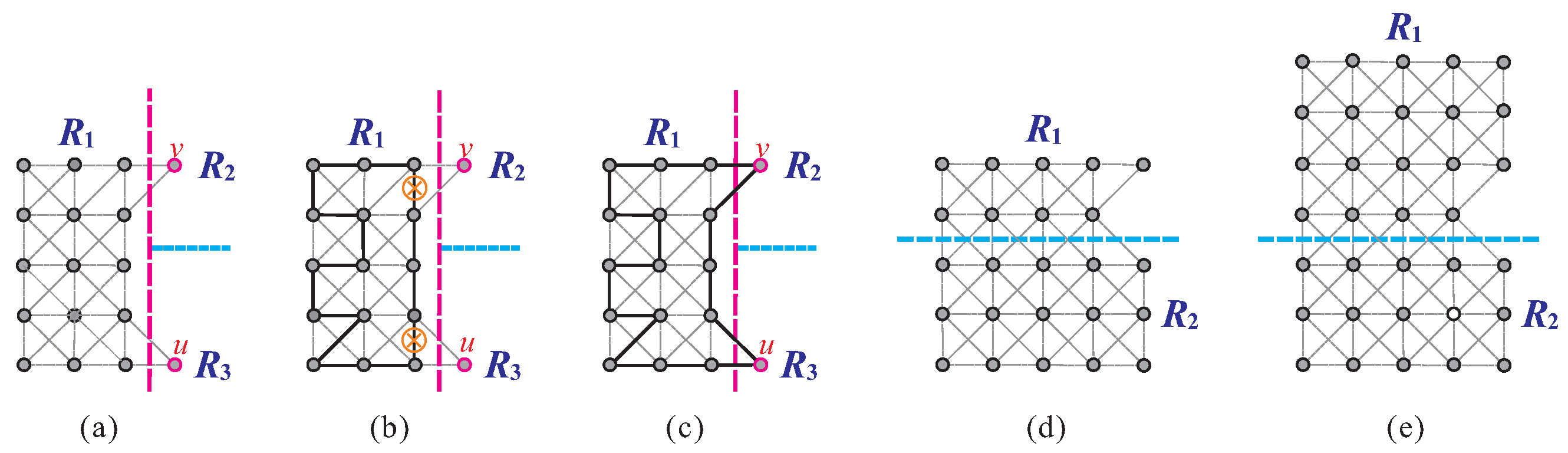
Case 1: $c=1$ and $d=1$. If $k>1$, then there exists a vertex $w\in V\left(C\right(m,n;k,l;c,d\left)\right)$ such that $deg\left(w\right)=1$. Thus, $k=1$. We make vertical and horizontal separations on $C(m,n;k,l;c,d)$ to obtain three disjoint rectangular supergrid subgraphs $R_1=R(a,n)$, $R_2=R(k,c)$, and $R_3=R(k,d)$, as depicted in Figure 9a. Assume that $v\in V\left(R_2\right)$ and $u\in V\left(R_3\right)$. By Lemma 1, $R_1$ contains a canonical Hamiltonian cycle $H{C}_1$ (see Figure 9b). We can place one flat face of $H{C}_1$ to face $R_2$ and $R_3$. Thus, there exists an edge $(w,z)\in H{C}_1$ such that $v\sim w$ and $v\sim z$. By Statement (3) of Proposition 1, v and $H{C}_1$ can be combined into a cycle $H{C}_2$. By the same argument, u can be merged into the cycle $H{C}_2$ to form a Hamiltonian cycle of $C(m,n;k,l;c,d)$, as shown in Figure 9c.

Case 2: $c⩾2$ or $d⩾2$. By symmetry, assume that $d⩾2$. We make a horizontal separation on $C(m,n;k,l;c,d)$ to obtain two disjoint supergrid subgraphs $R_1=L(m,c+l;k,l)$ and $R_2=R(m,d)$, as depicted in Figure 9d,e, where Figure 9d,e respectively, indicate the case of $c=1$ and $c⩾2$. By Theorem 2 (resp. Lemma 1), $R_1$ (resp. $R_2$) contains a Hamiltonian (resp. canonical Hamiltonian) cycle $H{C}_1$ (resp. $H{C}_2$) such that its one flat face is placed to face $R_2$ (resp. $R_1$). Then, there exist two edges $e_1=(u_1,u_2)\in H{C}_1$ and $e_2=(v_1,v_2)\in H{C}_2$ such that $e_1\approx e_2$; as shown in Figure 10a,b. By Statement (1) of Proposition 1, $H{C}_1$ and $H{C}_2$ can be combined into a Hamiltonian cycle of $C(m,n;k,l;c,d)$, as shown in Figure 10c,d.    □

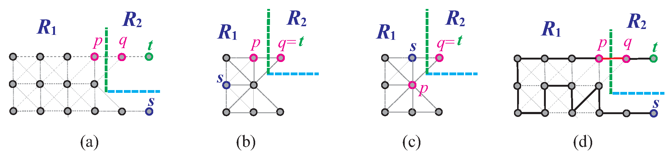
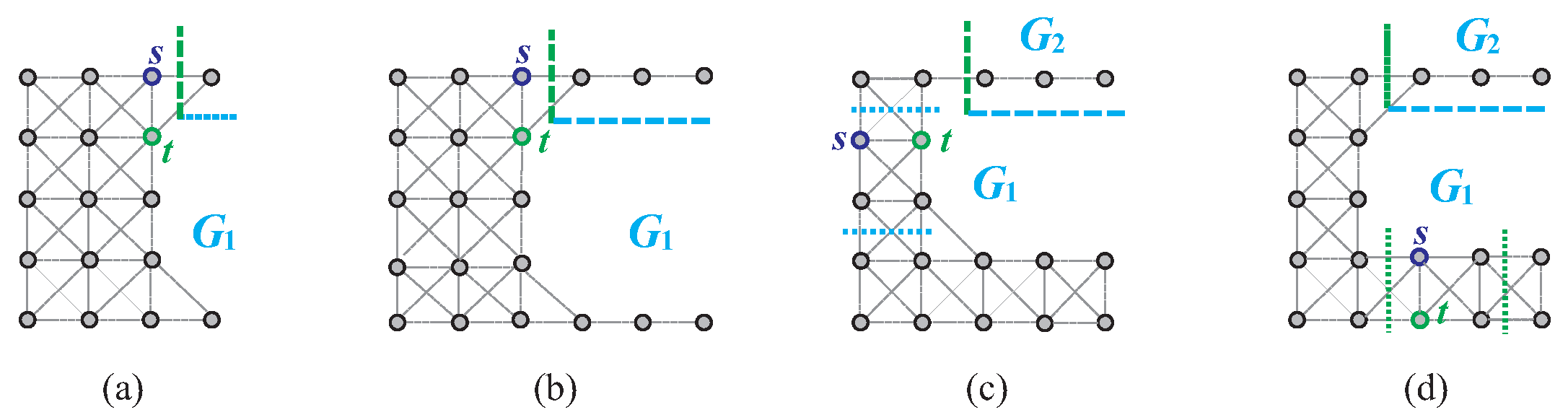
Now, we give the necessary and sufficient conditions for the existence of a Hamiltonian $(s,t)$-path in $C(m,n;k,l;c,d)$. In addition to condition (F1) (as depicted in Figure 11a,b) and (F3) (as depicted in Figure 11c), if $\left(C\right(m,n;k,l;$$c,d),s,t)$ satisfies one of the following conditions, then it contains no Hamiltonian $(s,t)$-path.

$\left(\mathrm{F}7\right)$

$m=3$, $a(=m-k)=2$, and $\left[\right(c=1$ and $\{s,t\}=\left\{\right(1,1),(2,2\left)\right\}$ or $\left\{\right(1,2),(2,1\left)\right\})$ or $(d=1$ and $\{s,t\}=\left\{\right(1,n),(2,n-1\left)\right\}$ or $\left\{\right(1,n-1),(2,n\left)\right\}\left)\right]$ (see Figure 11d).

$\left(\mathrm{F}8\right)$

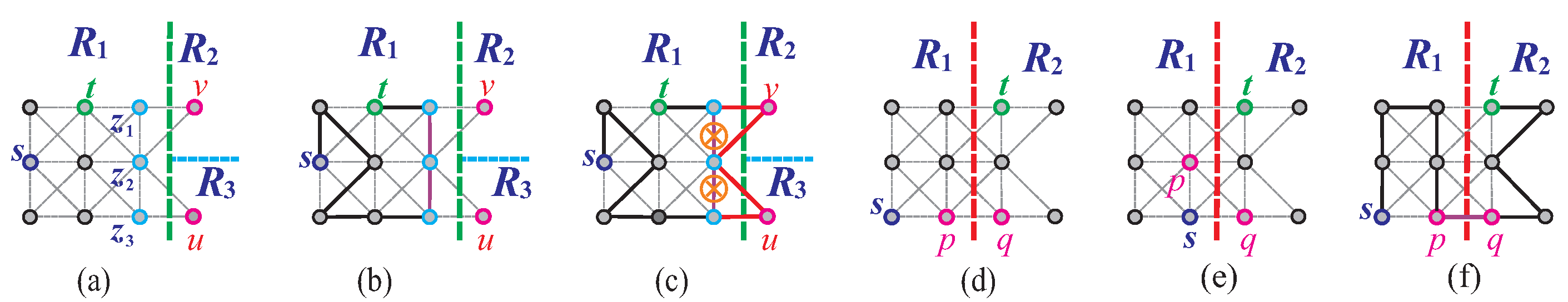
$n=3$, $k=c=d=1$, and

(1)

$a⩾2$, $s_x=t_x=m-1$, and $|s_y-t_y|=2$ (see Figure 11e); or

(2)

$a=2$, $s_x=1$, $t_x=2$, and $|s_y-t_y|=2$ (see Figure 11f); or

(3)

$a>2$, $s_x<m-1$, and $t=(m-1,2)$ (see Figure 11g).

$\left(\mathrm{F}9\right)$

$a(=m-k)=1$, and ($s_y,t_y⩽c$ or $s_y,t_y>c+l$) (see Figure 11h).

Lemma 7.

If $HP\left(C\right(m,n;k,l;c,d),s,t)$ exists, then $\left(C\right(m,n;k,l;c,d),s,t)$ does not satisfy conditions $\left(\mathrm{F}1\right)$, $\left(\mathrm{F}3\right)$, $\left(\mathrm{F}7\right)$, $\left(\mathrm{F}8\right)$, and $\left(\mathrm{F}9\right)$.

Proof. 

Assume that $\left(C\right(m,n;k,l;c,d),s,t)$ satisfies one of the conditions (F1), (F3), (F7), (F8), and (F9), then we show that $HP\left(C\right(m,n;k,l;c,d),s,t)$ does not exist. For conditions (F1) and (F3), it is clear (see Figure 11a–c). For condition (F7), by inspecting all cases of Figure 11d there exists no Hamiltonian $(s,t)$-path. For cases (1)–(2) of condition (F8), consider Figure 11e,f. Let v be a vertex depicted in these figures. Since $\{s,t,v\}$ is a vertex cut of $C(m,n;k,l;c,d)$, then $C(m,n;k,l;c,d)-\{s,t,v\}$ is disconnected and contains three (or two) components in which two components (or one component) consist of only one vertex. Hence, any path between s and t must pass through s or v twice. Therefore, $C(m,n;k,l;c,d)$ contains no Hamiltonian $(s,t)$-path. For case (3) of condition (F8), consider Figure 11g. A simple check shows that there is no Hamiltonian $(s,t)$-path in $C(m,n;k,l;c,d)$ containing both of vertices u and v. For condition (F9), consider Figure 11h. Let $v\in V\left(C\right(m,n;k,l;c,d)$ such that $v_x=1$ and $c+1⩽v_y⩽c+l$. Since $a=1$, v is a cut vertex of $C(m,n;k,l;c,d)$. Obviously, any path between s and t must pass through v two times. Therefore, $C(m,n;k,l;c,d)$ contains no Hamiltonian $(s,t)$-path.    □

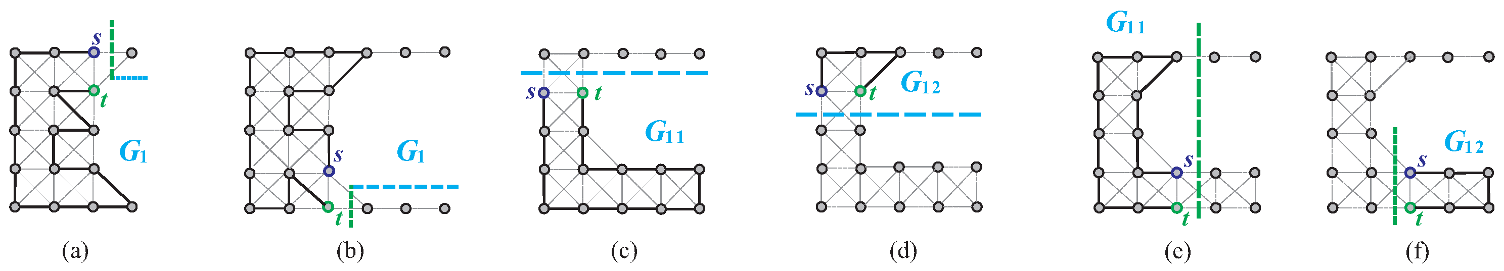
In the following, we will show that $C(m,n;k,l;c,d)$ has a Hamiltonian $(s,t)$-path when $\left(C\right(m,n;k,l;c,d),s,t)$ does not satisfy conditions (F1), (F3), (F7), (F8), and (F9). We consider the case of $a=1$ in Lemma 8 and the case of $a⩾2$ in Lemmas 9 and 10.

Lemma 8.

Assume that$a(=m-k)=1$and$\left(C\right(m,n;k,l;c,d),s,t)$does not satisfy conditions$\left(\mathrm{F}1\right)$, $\left(\mathrm{F}3\right)$, and$\left(\mathrm{F}9\right)$. Then$HP\left(C\right(m,n;k,l;c,d),s,t)$does exist.

Proof. 

Notice that, here, $(s_y⩽c$ and $t_y>c+l)$ or $(t_y⩽c$ and $s_y>c+l)$. If $s_y,t_y⩽c$, $s_y,t_y>c+l$, or $c+1⩽s_y\left(\mathrm{or}{t}_y\right)⩽c+l$, then $\left(C\right(m,n;k,l;c,d),s,t)$ satisfies condition (F1) or (F9). Without loss of generality, assume that $s_y⩽c$ and $t_y>c+l$. We make a horizontal separation on $C(m,n;k,l;c,d)$ to obtain two disjoint subgraphs $R_1=R(m,c)$, $R_2=L(m,n-c;k,l)$. Let $p\in V\left(R_1\right)$ and $q\in V\left(R_2\right)$ such that $p\sim q$, $q=(1,c+1)$, and $p=(1,c)$ if $s\ne (1,c)$; otherwise $p=(2,c)$ (see Figure 12a). Consider $(R_1,s,p)$. Condition (F1) holds, if

(i)

$c=1$, $k>1$, and $s_x\ne m$. Clearly, if this case holds, then $\left(C\right(m,n;k,l;c,d),$$s,t)$ satisfies condition (F1), a contradiction.

(ii)

$c=2$ and $s_x=p_x⩾2$. Clearly, in this case, $s_x=p_x=2$. It contradicts that $p=(1,c)$ when $s\ne (1,c)$.

Therefore, $(R_1,s,p)$ does not satisfy condition (F1). Now, consider $(R_2,q,t)$. Since $q_y=c+1$ and $t_y>c+l$, it is enough to show that $(R_2,q,t)$ does not satisfy condition (F1). Condition (F1) holds, if $d=1$, $k>1$, and $t_x\ne m$. Clearly, if this case holds, then $\left(C\right(m,n;k,l;c,d),s,t)$ satisfies condition (F1), a contradiction. Therefore, $(R_2,q,t)$ does not satisfy conditions (F1), (F3), and (F4). Since $(R_1,s,p)$ and $(R_2,q,t)$ do not satisfy conditions (F1), (F3), and (F4), by Lemma 3 and Theorem 1, there exist Hamiltonian $(s,p)$-path $P_1$ and Hamiltonian $(q,t)$-path $P_2$ of $R_1$ and $R_2$, respectively (see Figure 12b). Then, $P=P_1\Rightarrow P_2$ forms a Hamiltonian $(s,t)$-path of $C(m,n;k,l;c,d)$, as depicted in Figure 12c. □

Lemma 9.

Assume $c=d=1$, $a(=m-k)>1$, and $\left(C\right(m,n;k,l;c,d),s,t)$ does not satisfy conditions $\left(\mathrm{F}1\right)$, $\left(\mathrm{F}3\right)$, $\left(\mathrm{F}7\right)$, and $\left(\mathrm{F}8\right)$. Then $HP\left(C\right(m,n;k,l;$$c,d),s,t)$ does exist.

Proof. 

Depending on whether $n=3$, we consider the following cases:

Case 1: $n=3$. Notice that, here, if $k>1$, then $s_x=t_x=m$. If $k>1$ and $s_x\ne m$ and $t_x\ne m$, then $\left(C\right(m,n;k,l;c,d),s,t)$ satisfies (F1) or (F3). Consider the positions of s and t, as there are the following two subcases:

  Case 1.1: $s_x>a$ or $t_x>a$. Without loss of generality, assume that $t_x>a$ and $t_y=1$. We make a vertical and a horizontal separations on $C(m,n;k,l;c,d)$ to obtain two disjoint supergrid subgraphs $R_2=R(k,c)$ and $R_1=L(m,n;k,c+l)$, as depicted in Figure 13a–c. Let $p\in V\left(R_1\right)$ and $q\in V\left(R_2\right)$ such that $p\sim q$, $q=(a+1,1)$, and $p=(a,1)$ if $s\ne (a,1)$; otherwise $p=(a,2)$ (see Figure 13a–c). Here, if $\left|V\right(R_2\left)\right|=1$ (i.e., $k=1)$, then $q=t$. Consider $(R_1,s,p)$. Condition (F1) holds, if $a=2$ and $s_y=p_y⩾2$, or $p=(a,2)$ and $s=(a,3)$. Clearly, in any case, it contradicts that $p=(a,1)$ when $s\ne (a,1)$. Condition (F3) holds, if $k>1$ and $s_x⩽a$. If this case holds, then $\left(C\right(m,n;k,l;c,d),s,t)$ satisfies condition (F3), a contradiction. Condition (F4) holds, if $n=3$, $a=2$, $k=1$, $s=(1,n)$, and $p=(a,2)$. It contradicts that $p=(a,1)$ when $s\ne (a,1)$. Thus, $(R_1,s,p)$ does not satisfy conditions (F1), (F3), and (F4). Now, consider $(R_2,q,t)$. Since $q=(a+1,1)$ and $t=(m,1)$, clearly $(R_2,q,t)$ does not satisfy condition (F1). A Hamiltonian $(s,t)$-path of $C(m,n;k,l;c,d)$ can be constructed by similar arguments in proving Lemma 8, as shown in Figure 13d.

  Case 1.2: $s_x,t_x⩽a$. In this subcase, $k=1$ and hence $a=m-1$. If $k>1$, then $\left(C\right(m,n;k,l;c,d),s,t)$ satisfies (F3). Since $\left(C\right(m,n;k,l;c,d),s,t)$ does not satisfy condition (F8), $s_x\ne m-1$. There are two subcases:

    Case 1.2.1: $s_x,t_x<m-1$. Let $z_1=(m-1,1)$, $z_2=(m-1,2)$, and $z_3=(m-1,3)$. Let $e_1=(z_1,z_2)$ and $e_2=(z_2,z_3)$. We make a vertical and horizontal separations on $C(m,n;k,l;c,d)$ to obtain three disjoint rectangular supergrid subgraphs $R_1=R(a,n)$, $R_2=R(k,c)$, and $R_3=R(k,d)$; as depicted in Figure 14a. Assume that $v\in V\left(R_2\right)$ and $u\in V\left(R_3\right)$. By Lemma 6, where $a>2$, or Lemma 3, where $a=2$, $R_1$ contains a Hamiltonian $(s,t)$-path $P_1$ such that $e_1,e_2\in P_1$ (see Figure 14b). Then, $P_1$, u, v can be combined into a Hamiltonian $(s,t)$-path of $C(m,n;k,l;c,d)$ by Statement (3) of Proposition 1 (see Figure 14c).

    Case 1.2.2: $s_x<m-1$ and $t_x=m-1$. Since $\left(C\right(m,n;k,l;c,d),s,t)$ does not satisfy conditions (F1), (F7), and (F8), we have that (1) $t=(m-1,1)$ or $t=(m-1,3)$ if $m-1>2$, and (2) $s_y=t_y=1$ or $s_y=t_y=3$ if $m-1=2$. Thus, $t_y=1$ or $t_y=3$. By symmetry, assume that $t=(m-1,1)$. We make a vertical separation on $C(m,n;k,l;c,d)$ to obtain two disjoint supergrid subgraphs $R_1=R(m-2,n)$ and $R_2=C(2,n;k,l;c,d)$, as depicted in Figure 14d,e. Let $q\in V\left(R_2\right)$ and $p\in V\left(R_1\right)$ such that $p\sim q$, $q=(m-1,3)$, and $p=(m-2,3)$ if $s\ne (m-2,3)$; otherwise $p=(m-2,2)$ (see Figure 14d,e).

Notice that, here, if $s=(m-2,3)$, then $m⩾4$. If $m=3$ and $s=(m-2,3)$, then $\left(C\right(m,n;k,l;c,d),s,t)$ satisfies condition (F8). Consider $(R_2,q,t)$. Since $a=d=c=1$, $t=(m-1,1)$, and $q=(m-1,3)$, clearly $(R_2,q,t)$ does not satisfy conditions (F1), (F3), and (F9). Here, $(R_2,q,t)$ lies on Lemma 8. Now, consider $(R_1,s,p)$. Condition (F1) holds, if

(i)

$m-2=1$ and $s=(m-2,2)$. In this case, $\left(C\right(m,n;k,l;c,d),s,t)$ satisfies condition (F7), a contradiction.

(ii)

$m-2=2$ and $s_y=p_y=2$. Clearly if $s_y=2$, then $p_y=3$. Hence, $s_y\ne p_y$.

Therefore, $(R_1,s,p)$ does not satisfy condition (F1). By Lemmas 3 and 8, $R_1$ and $R_2$ contain Hamiltonian $(s,p)$-path $P_1$ and $(q,p)$-path $P_2$, respectively. Then, $P=P_1\Rightarrow P_2$ forms a Hamiltonian $(s,t)$-path of $C(m,n;k,l;c,d)$, as depicted in Figure 14f.

Case 2: $n>3$. Since $n>3$ and $c=d=1$, it follows that $l>1$. We make a horizontal separation on $C(m,n;k,l;c,d)$ to obtain two disjoint supergrid subgraphs $R_1=L(m,n-n_2;k,l_1)$ and $R_2=L(n_2,m;l_2,k)$, where $n_2=c+l-1$, $l_1=c+l-n_2$, and $l_2=l-l_1$ (see Figure 15a–c). Since $n_2=c+l-1$ and $d=1$, clearly $n-n_2=2$. Also since $n-n_2=2$ and $n>3$, it follows that $n_2⩾2$. Depending on the positions of s and t, there are the following two subcases:

  Case 2.1: $s,t\in R_1$ or $s,t\in R_2$. Without loss of generality, assume that $s,t\in R_2$. Here, $k=1$. If $k>1$, then $\left(C\right(m,n;k,l;c,d),s,t)$ satisfies condition (F3).

    Case 2.1.1: $(n_2>2)$ or $(n_2=2$ and $[(s_x\ne t_x)$ or $(s_x=t_x=1)\left]\right)$. Since $k=1$, it is enough to show that $(R_2,s,t)$ does not satisfy conditions (F1) and (F4). Condition (F1) holds, if

(i)

$2⩽s_x=t_x⩽a$. By assumption, this case does not occur.

(ii)

$a=2$ and $2⩽s_y=t_y⩽n_2$. Clearly if this case holds, then $\left(C\right(m,n;k,l;c,d),$$s,t)$ satisfies condition (F1), a contradiction.

Condition (F4) holds, if $a=2$, $n_2>2$, $s_x,t_x⩽2$, $s_y,t_y⩽2$, $s_x\ne t_x$, and $s_y\ne t_y$. Clearly, if this case holds, then $\left(C\right(m,n;k,l;c,d),s,t)$ satisfies condition (F7), a contradiction. Therefore, $(R_2,s,t)$ does not satisfy conditions (F1), (F3), and (F4). Since $(R_2,s,t)$ does not satisfy conditions (F1), (F3), and (F4). By Theorem 1, $R_2$ contains a Hamiltonian $(s,t)$-path $P_2$ in which one edge $e_2$ is placed to face $R_1$. By Theorem 2, $R_1$ contains a Hamiltonian cycle $H{C}_1$ such that its one flat face is placed to face $R_2$. Then, there exist two edges $e_1\in H{C}_1$ and $e_2\in P_2$ such that $e_1\approx e_2$ (see Figure 15d). By Statement (2) of Proposition 1, $P_2$ and $H{C}_1$ can be combined into a Hamiltonian $(s,t)$-path of $C(m,n;k,l;c,d)$. The construction of a such Hamiltonian path is depicted in Figure 15e.

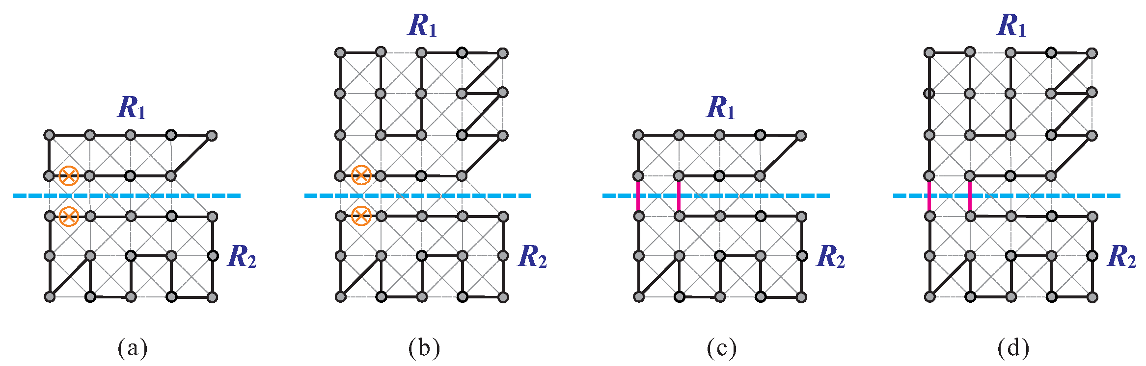
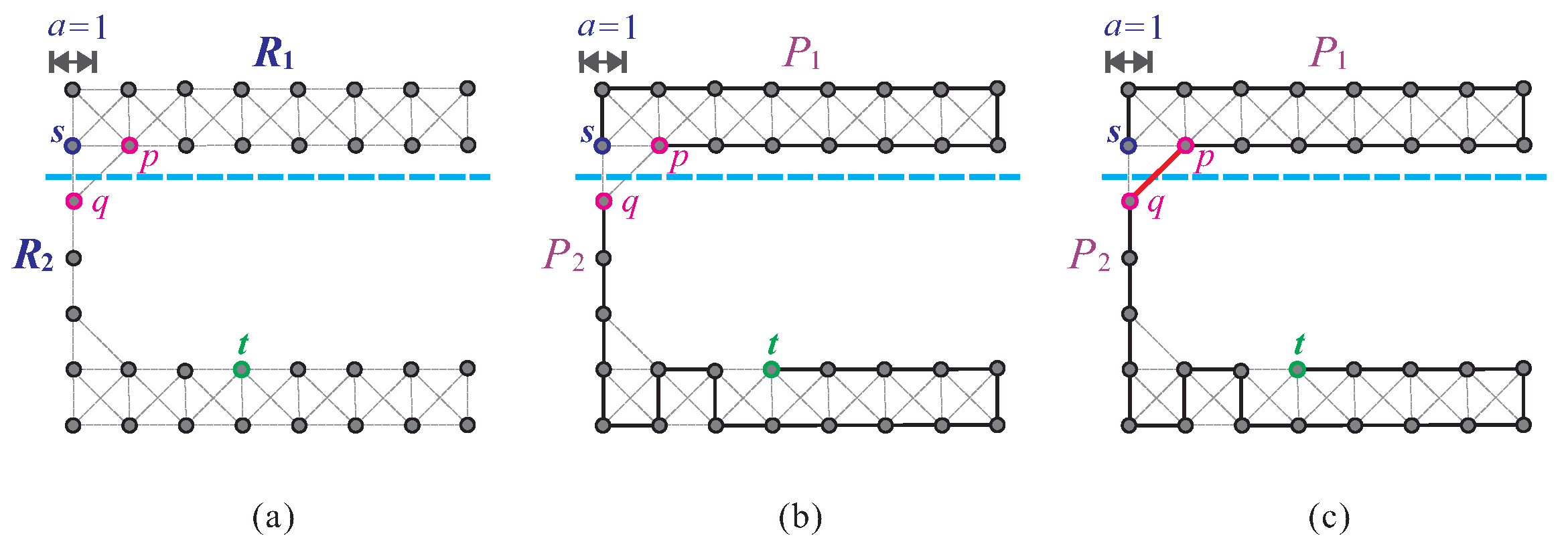
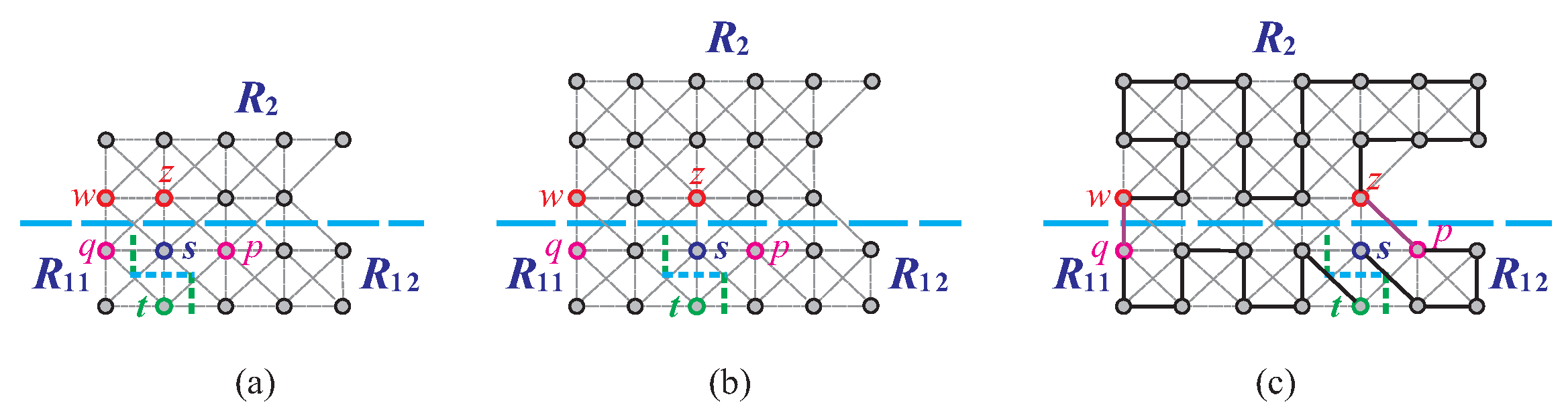
    Case 2.1.2: $n_2=2$ and $s_x,t_x>1$. In this case, $n=4$, $a>2$, $l=2$, and $2⩽s_x=t_x⩽a-1$. If $s_x=t_x=a$, then $\left(C\right(m,n;k,l;c,d),s,t)$ satisfies condition (F1). Depending on whether $a=3$, we consider the following two subcases:

      Case 2.1.2.1: $a=3$. In this subcase, we can construct a Hamiltonian $(s,t)$-path by the pattern shown in Figure 16a. Consider Figure 16a. Since $w=(1,3)$ and $z=(3,3)$, clearly $(R_1,w,z)$ does not satisfy conditions (F1), (F3), and (F4). Thus by Theorem 1, $R_1$ contains a Hamiltonian $(w,z)$-path $P_1$. For $(R_2,s,t)$, we can construct two paths $P_{21}$ and $P_{22}$ such that $P_{21}$ connects s and p, $P_{22}$ connects q and t, $V\left(P_{21}\right)\cap V\left(P_{22}\right)=\varnothing$, $V(P_{21}\cup P_{22})=V\left(R_2\right)$, $p\sim w$, and $q\sim z$, as shown in Figure 16a. Then, $P=P_{21}\Rightarrow P_1\Rightarrow P_{22}$ forms a Hamiltonian $(s,t)$-path of $C(m,n;k,l;c,d)$ (see Figure 16a).

      Case 2.1.2.2: $a>3$. We make a vertical separation on $R_2$ to obtain two disjoint subgraphs $R_{21}=R(m^{\prime },n_2)$ and $R_{22}=L(n_2,m-m^{\prime };1,1)$, where $m^{\prime }=s_x$ if $s_x<a-1$; otherwise $m^{\prime }=s_x-1$; as shown in Figure 16b,c. First, let $s,t\in R_{21}$ and consider Figure 16b. Clearly since $s_x=t_x=m^{\prime }$, $(R_{21},s,t)$ does not satisfy condition (F1). By Lemma 3, $R_{21}$ contains a canonical Hamiltonian $(s,t)$-path $P_{21}$. Then, there exists one edge $e_{21}\in P_{21}$ that is placed to face $R_1$. By Theorem 2, $R_{22}$ and $R_1$ contain Hamiltonian cycle $H{C}_{22}$ and $H{C}_1$, respectively. Using the algorithm of [17], we can construct $H{C}_{22}$ and $H{C}_1$ to satisfy that one flat face of $H{C}_1$, which is placed to face $R_{21}$ and $R_{22}$, and one flat face of $H{C}_{22}$, which is placed to face $R_1$ (see Figure 16d). Then, there exist four edges $e_1,e_2\in H{C}_1$, $e_{21}\in P_{21}$, and $e_{22}\in H{C}_{22}$ such that $e_1\approx e_{21}$ and $e_2\approx e_{22}$. By Statements (1) and (2) of Proposition 1, $P_{21}$, $H{C}_1$, and $H{C}_{22}$ can be combined into a Hamiltonian $(s,t)$-path of $C(m,n;k,l;c,d)$. The construction of a such Hamiltonian path is depicted in Figure 16e. Now, let $s,t\in R_{22}$ and consider Figure 16c. Since $s_x=t_x=1$ and $s_x,t_x<a$ (in $R_{22}$), it is clear that $(R_{22},s,t)$ does not satisfy conditions (F1), (F3), and (F4). By similar arguments in proving $s,t\in R_{21}$, a Hamiltonian $(s,t)$-path of $C(m,n;k,l;c,d)$ can be constructed (see Figure 16f).

  Case 2.2: ($s\in R_1$ and $t\in R_2$) or ($t\in R_1$ and $s\in R_2$). Without loss of generality, assume that $t\in R_1$ and $s\in R_2$. Let $q\in V\left(R_1\right)$ and $p\in V\left(R_2\right)$ such that $p\sim q$, where

$$\left\{\begin{array}{cc}p=(1,n_2)\mathrm{and}q=(1,n_2+1),\hfill & \mathrm{if}s\ne (1,n_2)\mathrm{and}t\ne (1,n_2+1);\hfill \\ p=(2,n_2)\mathrm{and}q=(2,n_2+1),\hfill & \mathrm{if}s=(1,n_2)\mathrm{and}t=(1,n_2+1);\hfill \\ p=(2,n_2)\mathrm{and}q=(1,n_2+1),\hfill & \mathrm{if}s=(1,n_2)\mathrm{and}t\ne (1,n_2+1);\hfill \\ p=(1,n_2)\mathrm{and}q=(2,n_2+1),\hfill & \mathrm{otherwise}.\hfill \end{array}\right.$$

Consider $(R_2,s,p)$ and $(R_1,q,t)$. Condition (F1) holds, if

(i)

$(n_2=2$ and $s_x=p_x=2)$ or $(n-n_2=2$ and $q_x=t_x=2)$. Obviously in this case, $s_x=p_x=2$ and $q_x=t_x=2$. It contradicts that $p_x=q_x=1$ when $s_x\ne 1$ and $t_x\ne 1$.

(ii)

$k>1$ and $a<s_x,t_x<m$. If this case holds, then $\left(C\right(m,n;k,l;c,d),s,t)$ satisfies condition (F1), a contradiction.

Condition (F3) holds, if $k>1$ and $s_x,t_x⩽a$. If this case holds, then $\left(C\right(m,n;$$k,l;c,d),s,t)$ satisfies condition (F3), a contradiction. Condition (F4) holds, if $a=2$ and $\left[\right(n_2>2$ and $s_y,p_y⩽2)$ or $(n-n_2>2$ and $q_y,t_y⩾n-1\left)\right]$. A simple check shows that these cases do not occur. Therefore, $(R_2,s,p)$ and $(R_1,q,t)$ do not satisfy conditions (F1), (F3), and (F4). A Hamiltonian $(s,t)$-path of $C(m,n;k,l;c,d)$ can be constructed by similar arguments in proving Lemma 8. Notice that, here, $R_1$ and $R_2$ are L-shaped supergrid graphs.    □

Lemma 10.

Assume $a(=m-k)>1$, $(c>1$ or $d>1)$, and $\left(C\right(m,n;k,l;c,d),$$s,t)$ does not satisfy conditions $\left(\mathrm{F}1\right)$, $\left(\mathrm{F}3\right)$, $\left(\mathrm{F}7\right)$, and $\left(\mathrm{F}8\right)$. Then $HP\left(C\right(m,n;$$k,l;c,d),s,t)$ does exist.

Proof. 

Without loss of generality, assume that $d>1$. Since $d>1$, $c⩾1$, and $l⩾1$, thus $n⩾4$. We make a horizontal separation on $C(m,n;k,l;c,d)$ to obtain two disjoint supergrid subgraphs $R_2=L(n_2,m;l,k)$ and $R_1=R(m,n-n_2)$, where $n_2=c+l$ and $n-n_2=d$ (see Figure 17a,b). Since $n⩾4$, $n_2=c+l$, $c,l⩾1$, and $d>1$, it follows that $n-n_2,n_2⩾2$. Depending on the positions of s and t, there are the following three subcases:

Case 1: $s,t\in R_1$. In this case, ($c>1$) or ($c=1$ and $k=1$). If $c=1$ and $k>1$, then $\left(C\right(m,n;k,l;c,d),s,t)$ satisfies condition (F3), a contradiction. Depending on the size of $n-n_2$, we consider the following two subcases:

  Case 1.1: ($n-n_2>2$) or ($n-n_2=2$ and $[(s_x\ne t_x)$, $(s_x=t_x=1)$, or $(s_x=t_x=m)]$). In this subcase, $\{s,t\}$ is not a vertex cut of $R_1$. Then, $(R_1,s,t)$ does not satisfy condition (F1). By Lemma 3, $R_1$ contains a canonical Hamiltonian $(s,t)$-path $P_1$. Using the algorithm of [12], we can construct a Hamiltonian $(s,t)$-path $P_1$ of $R_1$ in which one edge $e_1$ is placed to face $R_2$. By Theorem 2, $R_2$ contains a Hamiltonian cycle $H{C}_2$. Using the algorithm of [17], we can construct $H{C}_2$ such that its one flat face is placed to face $R_1$. Then, there exist two edges $e_1\in P_1$ and $e_2\in H{C}_2$ such that $e_1\approx e_2$ (see Figure 17c). By Statement (2) of Proposition 1, $P_1$ and $H{C}_2$ can be combined into a Hamiltonian $(s,t)$-path of $C(m,n;k,l;c,d)$. The construction of a such Hamiltonian path is depicted in Figure 17d.

  Case 1.2: $n-n_2=2$ and $1<s_x=t_x<m$. In this subcase, $\{s,t\}$ is a vertex cut of $R_1$. Notice that, here, $s_x,t_x⩽a$. If $s_x,t_x>a$ and $k>1$, then $\left(C\right(m,n;k,l;c,d),s,t)$ satisfies condition (F1). Without loss of generality, assume that $s_y<t_y$. We make a vertical and a horizontal separations on $R_1$ to obtain two disjoint supergrid subgraphs $R_{11}=L(s_x,n-n_2;1,1)$ and $R_{12}=R_1-R_{11}$. Let $p\in V\left(R_{12}\right)$, $q\in V\left(R_{11}\right)$, and $w,z\in V\left(R_2\right)$ such that $p\sim z$, $q\sim w$, $q=(1,n_2+1)$, $w=(1,n_2)$, $p=(s_x+1,n_2+1)$, and $z=(s_x,n_2)$ (see Figure 18a,b). A simple check shows that $(R_{12},s,p)$, $(R_2,z,w)$, and $(R_{11},q,t)$ do not satisfy conditions (F1), (F3), and (F4). Thus, by Theorem 1, $R_{12}$, $R_2$, and $R_{11}$ contain a Hamiltonian $(s,p)$-path $P_{12}$, Hamiltonian $(z,w)$-path $P_2$, and Hamiltonian $(q,t)$-path $P_{11}$, respectively. Then, $P=P_{12}\Rightarrow P_2\Rightarrow P_{11}$ forms a Hamiltonian $(s,t)$-path of $C(m,n;k,l;c,d)$. The construction of a such Hamiltonian path is depicted in Figure 18c.

Case 2: $s,t\in R_2$. A Hamiltonian $(s,t)$-path of $\left(C\right(m,n;k,l;c,d)$ can be constructed by similar arguments in proving Case 2.1 of Lemma 9. Notice that, in this case, $R_1$ is a rectangular supergrid graph.

Case 3: ($s\in R_1$ and $t\in R_2$) or ($s\in R_2$ and $t\in R_1$). A Hamiltonian $(s,t)$-path of $\left(C\right(m,n;k,l;c,d)$ can be constructed by similar arguments in proving Case 2.2 of Lemma 9. Notice that, in this case, $R_1$ is a rectangular supergrid graphs.    □

It immediately follows from Lemmas 7–10 that the following theorem holds true.

Theorem 5.

$HP\left(C\right(m,n;k,l;c,d),s,t)$ does exist if and only if $\left(C\right(m,n;k,l;$$c,d),s,t)$ does not satisfy conditions $\left(\mathrm{F}1\right)$, $\left(\mathrm{F}3\right)$, $\left(\mathrm{F}7\right)$, $\left(\mathrm{F}8\right)$, and $\left(\mathrm{F}9\right)$.

4. The Longest $(\mathbf{s},\mathbf{t})$-Paths in $\mathbf{C}$-Shaped Supergrid Graphs

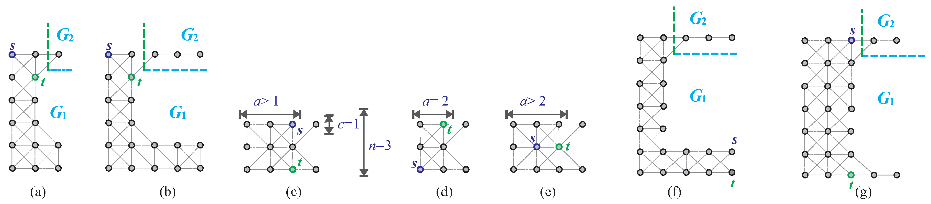
In this section, first for the cases where $HP\left(C\right(m,n;k,l;c,d),s,t)$ does not exist, we give the upper bounds on the lengths of the longest paths between s and t. Then, we show that these upper bounds are equal to the lengths of the longest path between s and t. Notice that the isomorphic cases are omitted. In the following, we use $\widehat{L}(G,s,t)$ to denote the length of the longest $(s,t)$-paths and $\widehat{U}(G,s,t)$ to indicate the upper bound on the length of the longest $(s,t)$-paths, where G is a rectangular, L-shaped, or C-shaped supergrid graph. By the length of a path we mean the number of vertices visited by the path. These upper bounds are given in Lemmas 11–13.

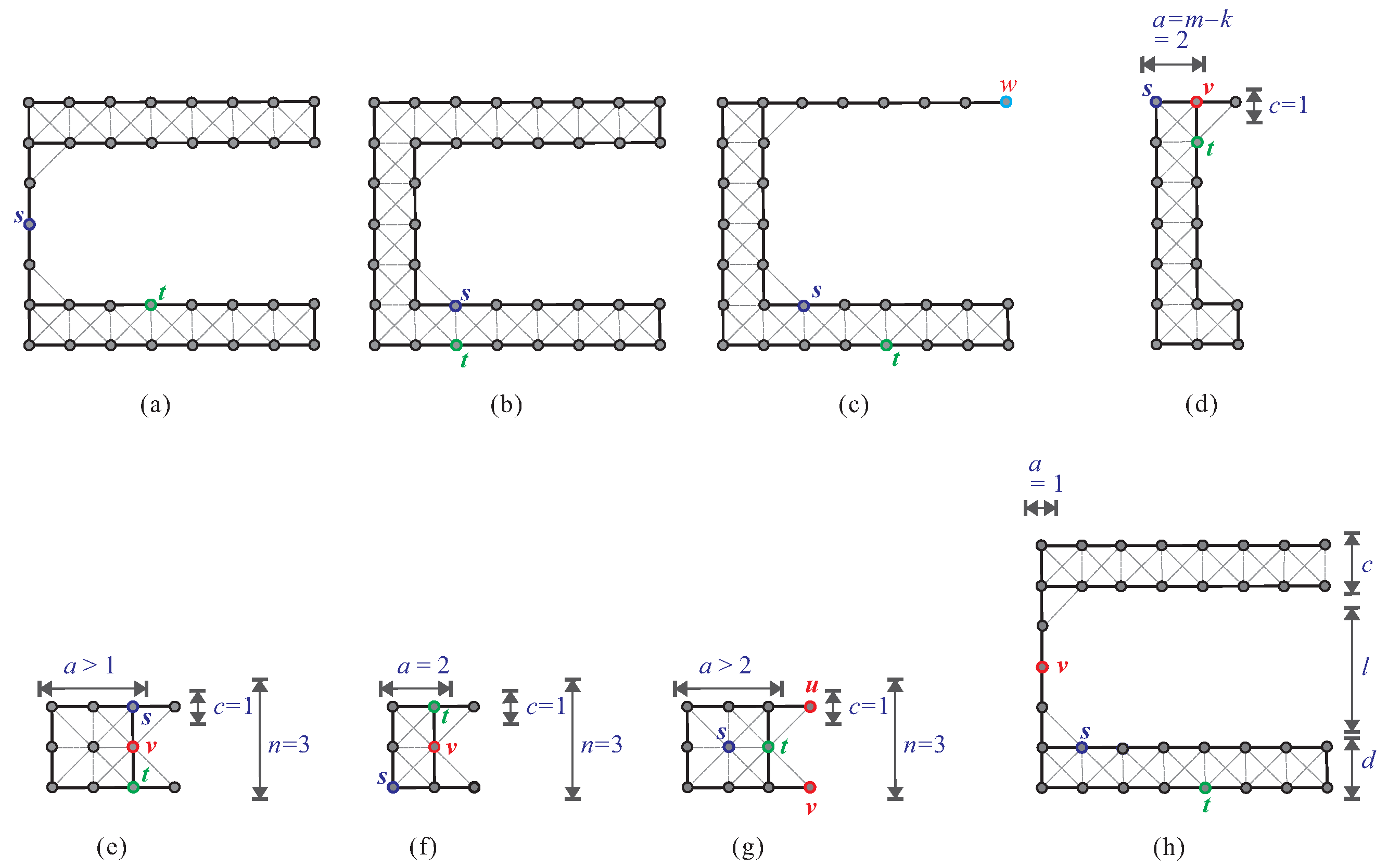
We first consider the case of $a=1$, where $a=m-k$. In this case, $\left(C\right(m,n;k,l;c,d),s,t)$ may satisfy conditions (F1), (F3), or (F9). We compute the upper bound of the longest $(s,t)$-path in this case as the following lemma.

Lemma 11.

Let $a=1$ and $w=(1,c+1)$. Assume that $C(m,n;k,l;c,d),s,t)$ satisfies one of the conditions $\left(\mathrm{F}1\right)$, $\left(\mathrm{F}3\right)$, and $\left(\mathrm{F}9\right)$. Then, the following conditions hold:

$\left(\mathrm{UB}1\right)$

If $s_y,t_y>c$ (resp., $s_y,t_y⩽c$), then the length of any $(s,t)$-path cannot exceed $\widehat{L}(G_1,s,t)$, where $G_1=L(m,n-c;k,l)$ (resp., $G_1=L(c+1,m;1,k)$) (see Figure 19a,b).

$\left(\mathrm{UB}2\right)$

If $(s_y⩽c$ and $t_y>c)$ or $(t_y⩽c$ and $s_y>c)$, without loss of generality assume that $s_y⩽c$, then the length of any $(s,t)$-path cannot exceed $\widehat{L}(G_2,s,z)+\widehat{L}(G_1,w,t)$, where $G_2=R(m,c)$, $G_1=L(m,n-c;k,l)$, and $z=(1,c)$ if $s\ne (1,c)$; otherwise $z=(2,c)$ (see Figure 19c,d).

Proof. 

The proof is straightforward, see Figure 19.    □

Next, we consider the case of $a⩾2$. In this case, $\left(C\right(m,n;k,l;c,d),s,t)$ may satisfy conditions (F1), (F3), (F7), or (F8). Depending on the sizes of c and d, we consider the subcases of (1) $c,d⩾2$ and (2) $c=1$ or $d=1$. Consider that $c,d⩾2$. Then, $\left(C\right(m,n;k,l;c,d),s,t)$ does not satisfy conditions (F3), (F7), and (F8). Thus, $\left(C\right(m,n;k,l;c,d),s,t)$ may satisfy condition (F1) only. We can see that s or t is not a cut vertex when $a,c,d⩾2$. Thus, $\{s,t\}$ is a vertex cut when $\left(C\right(m,n;k,l;c,d),s,t)$ satisfies condition (F1). We can see from the structure of $C(m,n;k,l;c,d)$ that a, c, or d is equal to 2 if $\{s,t\}$ is a vertex cut. The following lemma shows the upper bound of the longest $(s,t)$-path under that $a,c,d⩾2$ and $\left(C\right(m,n;k,l;c,d),s,t)$ satisfies condition (F1).

Lemma 12.

Assume that $a,c,d⩾2$ and $\{s,t\}$ is a vertex cut. Then, the following conditions hold:

$\left(\mathrm{UB}3\right)$

If $a=2$ and $c+1⩽s_y=t_y⩽c+l$, then the length of any $(s,t)$-path cannot exceed $max\{\widehat{L}(G_{11},s,t),\widehat{L}(G_{12},s,t)\}$, where $G_{11}=L(m,n^{\prime };k,l^{\prime })$, $G_{12}=L(s_y,m;k^{\prime },k)$, $n^{\prime }=n-s_y+1$, $l^{\prime }=n^{\prime }-d$, and $k^{\prime }=s_y-1$ (see Figure 20a,b).

$\left(\mathrm{UB}4\right)$

If $k⩾2$, $a+1⩽s_x,t_x⩽a+k-1(=m-1)$, and $\left[\right(c=2$ and $s_y,t_y⩽c)$ or $(d=2$, and $s_y,t_y⩾c+l\left)\right]$, without loss of generality assume that $d=2$ and $s_y,t_y⩾c+l$, then the length of any $(s,t)$-path cannot exceed $\widehat{L}(G_1,s,t)+\left|V\left(G_2\right)\right|=\widehat{L}(G_1,s,t)+k\times c$, where $G_1=L(m,n;k,l+c)$ and $G_2=R(k,c)$ (see Figure 20c,d).

Proof. 

Consider Figure 20a,b. Removing s and t clearly disconnects $C(m,n;$$k,l;c,d)$ into two components $G_1$ and $G_2$. Thus, a simple path between s and t can only go through one of these components. Therefore, its length cannot exceed the size of the largest component. Notice that, for (UB4), the length of any path between s and t is equal to $max\{\widehat{L}(G_1,s,t)+|V\left(G_2\right)|,2\times (m-s_x+1)\}$ (see Figure 20c,d). Since $a,c>1$, it is obvious that the length of any $(s,t)$-path cannot exceed $\widehat{L}(G_1,s,t)+\left|V\left(G_2\right)\right|=\widehat{L}(G_1,s,t)+k\times c$.    □

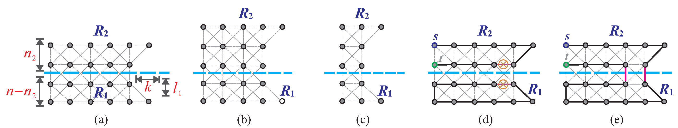
In the following, we will consider that $a⩾2$, and ($c=1$ or $d=1$). Without loss of generality, assume that $c=1$. We first make a horizontal and a vertical separation on $C(m,n;k,l;c,d)$ to obtain two disjoint subgraphs $G_1=L(m,n;k,l+c)$ and $G_2=R(m-a,c)$, as depicted in Figure 21a, where $a⩾2$, $c=1$, and $G_2$ is a path graph. Depending the locations of s and t, we consider the following cases:

Case I: $s,t\in G_2$. In this case, $k>1$, $s_y=t_y=1$, and $a+1⩽s_x,t_x⩽m$. Then, $\left(C\right(m,n;k,l;c,d),s,t)$ may satisfy conditions (F1) or (F3), as depicted in Figure 21b.

Case II: $s\in G_1$ and $t\in G_2$. In this case, $\left(C\right(m,n;k,l;c,d),s,t)$ may satisfy conditions (F1) or (F3), as depicted in Figure 21c.

Case III: $s,t\in G_1$. In this case, $\left(C\right(m,n;k,l;c,d),s,t)$ may satisfy conditions (F1), (F3), (F7), or (F8), as depicted in Figure 21d. If $d=1$, $s_y=t_y=n$, and $a+1⩽s_x,t_x⩽m$, then it is the same as Case I. Depending on whether $(G_1,s,t)$ satisfies condition (F1), there are the following three subcases:

  Case III.1: s or t is a cut vertex of $G_1$. In this subcase, $d=1$, and it is the same as Cases I or II.

  Case III.2: $\{s,t\}$ is a vertex cut of $G_1$. Consider the following subcases:

    Case III.2.1: $\{s,t\}=\left\{\right(a,1),(a,2\left)\right\}$. In this subcase, $k=1$ or $k>1$, as shown in Figure 22a,b. If $k>1$, then $\left(C\right(m,n;k,l;c,d),s,t)$ satisfies conditions (F1) and (F3); otherwise it satisfies condition (F1).

    Case III.2.2: $a=2$, $s_y=t_y$, and $c+1⩽s_x,t_x⩽c+l$. In this subcase, it is similar to condition (UB3) in Lemma 12 (see Figure 22c).

    Case III.2.3: $d=2$, $k>1$, $a<s_x=t_x<m$, and $n-1⩽s_y,t_y⩽n$. In this subcase, it is similar to condition (UB4) in Lemma 12 (see Figure 22d).

  Case III.3: $(G_1,s,t)$ does not satisfy condition (F1). In this subcase, s and t are not cut vertices and $\{s,t\}$ is not a vertex cut of $G_1$. Then, $\left(C\right(m,n;k,l;c,d),s,t)$ may satisfy conditions (F3), (F7), or (F8). Depending on the size of k, we consider the following subcases:

    Case III.3.1: $k=1$. In this subcase, $\left(C\right(m,n;k,l;c,d),s,t)$ may satisfy conditions (F7) and (F8), as follows:

      Case III.3.1.1: $\left(C\right(m,n;k,l;c,d),s,t)$ satisfies condition (F7). In this subcase, $a=2$ and $\left[\right(c=1$ and $\{s,t\}=\left\{\right(1,1),(2,2\left)\right\}$ or $\left\{\right(1,2),(2,1\left)\right\})$ or $(d=1$ and $\{s,t\}=\left\{\right(1,n),(2,n-1\left)\right\}$ or $\left\{\right(1,n-1),(2,n\left)\right\}\left)\right]$ (see Figure 23a).

      Case III.3.1.2: $\left(C\right(m,n;k,l;c,d),s,t)$ satisfies condition (F8). In this subcase, $n=3$ and $k=c=d=1$ (see Figure 23c–e).

    Case III.3.2: $k>1$. In this subcase, $\left(C\right(m,n;k,l;c,d),s,t)$ satisfies condition (F3) but it does not satisfy condition (F1). There are the following subcases:

      Case III.3.2.1: $a=2$ and $\left[\right(c=1$ and $\{s,t\}=\left\{\right(1,1),(2,2\left)\right\}$ or $\left\{\right(1,2),(2,1\left)\right\})$ or $(d=1$ and $\{s,t\}=\left\{\right(1,n),(2,n-1\left)\right\}$ or $\left\{\right(1,n-1),(2,n\left)\right\}\left)\right]$. In this subcase, it is the same as Case III.3.1.1 (see Figure 23b).

      Case III.3.2.2: $(c=1$ and $\{s,t\}\ne \left\{\right(1,1),(2,2\left)\right\}$ and $\left\{\right(1,2),(2,1\left)\right\})$ or $(d=1$ and $\{s,t\}\ne \left\{\right(1,n),(2,n-1\left)\right\}$ and $\left\{\right(1,n-1),(2,n\left)\right\})$ (see Figure 23e,f).

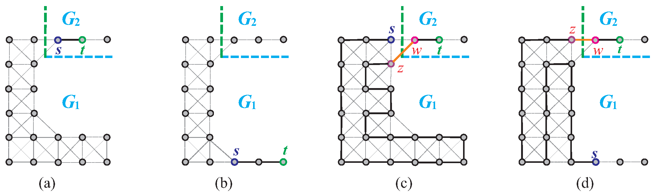
Based on the above cases, we compute the upper bounds of the longest $(s,t)$-paths on $\left(C\right(m,n;k,l;c,d),s,t)$ under that $a⩾2$ and $c=1$ as the following lemma.

Lemma 13.

Assume that $a⩾2$ and $c=1$. Let $w=(a+1,1)$. Then, the following conditions hold:

$\left(\mathrm{UB}5\right)$

If $k>1$, $a+1⩽s_x,t_x⩽m$, and ($s_y=t_y=1$ or $s_y=t_y=n$), then the length of any $(s,t)$-path cannot exceed $t_x-s_x+1$ (see Figure 24a,b, and refer to Case I and Case III.1).

$\left(\mathrm{UB}6\right)$

If $t_x>1$, $t_y=1$, and $[(s_x⩽a)$ or $(s_x>a$ and $s_y>c+l\left)\right]$, then the length of any $(s,t)$-path cannot exceed $\widehat{L}(G_1,s,z)+\widehat{L}(G_2,w,t)$, where $G_1=L(m,n;k,l+c)$, $G_2=R(k,c)$, and $z=(a,1)$ if $s\ne (a,1)$; otherwise $z=(a,2)$ (see Figure 24c,d, and refer to Cases II and III.1).

$\left(\mathrm{UB}7\right)$

If $\{s,t\}=\left\{\right(a,1),(a,2\left)\right\}$ (resp., $d=1$ and $\{s,t\}=\left\{\right(a,n-1),(a,n\left)\right\}$), then the length of any $(s,t)$-path cannot exceed $\widehat{L}(G_1,s,t)$, where $G_1=L(m,n;k,l+c)$ (resp., $G_1=L(n,m;l+d,k)$) (see Figure 25a,b, and refer to Case III.2.1).

$\left(\mathrm{UB}8\right)$

If $a=2$, $s_y=t_y$, and $c+1⩽s_y,t_y⩽c+l$, then the length of any $(s,t)$-path cannot exceed $max\{\widehat{L}(G_{11},s,t),\widehat{L}(G_{12},s,t)\}$, where $G_{11}=L(m,n^{\prime };k,l^{\prime })$, $G_{12}=L(s_y,m;k^{\prime },k)$, $n^{\prime }=n-s_y+1$, $l^{\prime }=n^{\prime }-d$, and $k^{\prime }=s_y-1$ (see Figure 25c,d, and refer to Case SIII.2.2).

$\left(\mathrm{UB}9\right)$

If $d=2$, $k>1$, $a<s_x=t_x<m$, and $n-1⩽s_y,t_y⩽n$, then the length of any $(s,t)$-path cannot exceed $max\{\widehat{L}(G_{11},s,t),\widehat{L}(G_{12},s,$$t\left)\right\}$, where $G_{11}=C(m^{\prime },n;k^{\prime },l;c,d)$, $G_{12}=R(m-m^{\prime }+1,d)$, $m^{\prime }=s_x$, and $k^{\prime }=m^{\prime }-a$ (see Figure 25e,f, and refer to Case III.2.3).

$\left(\mathrm{UB}10\right)$

If $a=2$ and $\left(\right\{s,t\}=\{(1,1),(2,2)\}$ or $\left\{\right(1,2),(2,1\left)\right\})$ (resp., $d=1$ and $\{s,t\}=\left\{\right(1,n),(2,n-1\left)\right\}$ or $\left\{\right(1,n-1),(2,n\left)\right\}$), then the length of $(s,t)$-path cannot exceed $\widehat{L}(G_1,s,t)$, where $G_1=L(m,n;k,l+c)$ (resp., $G_1=L(n,m;l+d,k)$) (see Figure 26a–c, and refer to Case III.3.1.1 and Case III.3.2.1).

$\left(\mathrm{UB}11\right)$

If $\left(C\right(m,n;k,l;c,d),s,t)$ satisfies condition (F8), then the length of $(s,t)$-path cannot exceed $\widehat{L}(G_1,s,t)$, where $G_1=L(m,n;k,l+c)$ (see Figure 26d–f, and refer to Case III.3.1.2).

$\left(\mathrm{UB}12\right)$

If $\left(C\right(m,n;k,l;c,d),s,t)$ does not satisfy condition (F1), $k>1$, and $\left[\right(a>2)$ or $(a=2,\{s,t\}\ne \{(1,1),(2,2)\}$ and $\left\{\right(1,2),(2,1\left)\right\}\left)\right]$ (resp., $d=1$ and $\{s,t\}\ne \left\{\right(1,n),(2,n-1\left)\right\}$ and $\left\{\right(1,n-1),(2,n\left)\right\}$), then the length of any $(s,t)$-path cannot exceed $\widehat{L}(G_1,s,t)+1$, where $G_1=L(m,n;k,l+c)$(resp., $G_1=L(n,m;l+d,k)$) (see Figure 26g,h, and refer to Case III.3.2.2).

Proof. 

For (UB5), consider Figure 24a,b. There is only one single path between s and t that has the specified. For (UB6), consider Figure 24c,d. Since $c=1$ and w is a cut vertex, it is clear that the length of any $(s,t)$-path cannot exceed $\widehat{L}(G_1,s,z)+\widehat{L}(G_2,w,t)$.

For (UB7), consider Figure 25a,b. In Figure 25a,b, $\{s,t\}$ is a vertex cut and hence removing s and t clearly disconnects $C(m,n;k,l;c,d)$ into two components. Thus, a simple path between s and t can only go through one of these components. Therefore, its length cannot exceed the size of the largest component. Since $c=1$, the larger component will be $G_1=L(m,n;k,l+c)$. For (UB8) and (UB9), consider Figure 25c–f. The computations of their upper bounds are the same as (UB7), and (UB3) in Lemma 12.

For (UB10), consider Figure 26a–c. A simple check shows that the length of any $(s,t)$-path cannot exceed $\widehat{L}(G_{\mathrm{a}},s,p)+\widehat{L}(G_{\mathrm{b}},q,t)=\widehat{L}\left(L\right(m,n;$$k,l+c),s,t)$, where $G_{\mathrm{a}}$, $G_{\mathrm{b}}$, p, q are defined in Figure 26a–c. For (UB11), consider Figure 26d–f. In Figure 26d–f, let $r=(a,1)$ and $z=(a,2)$, where $r,z$ may be one of s and t. Removing r and z clearly disconnects $C(m,n;k,l;c,d)$ into two components and a simple path between s and t can only go through a component that contains s, t, r, and z. Since the one disjoint component contains only one vertex, the upper bound of the longest $(s,t)$-path will be $\widehat{L}(L(m,n;k,l+c),s,t)$. For (UB12), consider Figure 26g,h. Since w is a cut vertex, we can easily show that the length of any path between s and t cannot exceed $\widehat{L}(G_1,s,t)+1$, where $G_1=L(m,n;k,l+c)$ or $L(n,m;l+d,k)$.    □

Assume that condition (C0) is defined as follows:

$\left(\mathrm{C}0\right)$

$\left(C\right(m,n;k,l;c,d),s,t)$ does not satisfy any of conditions (F1), (F3), (F7), (F8), and (F9).

Clearly $\left(C\right(m,n;k,l;c,d),s,t)$ must satisfy one of conditions (C0), (UB1), (UB2), (UB3), (UB4), (UB5), (UB6), (UB7), (UB8), (UB9), (UB10), (UB11), and (UB12). If $\left(C\right(m,n;k,l;c,d),s,$$t)$ satisfies (C0), then $\widehat{U}(C(m,n;k,l;c,d),$$s,t)=|V\left(C\right(m,n;$$k,l;c,d\left)\right)|=mn-kl$. Otherwise, $\widehat{U}(C(m,n;k,l;c,d),s,t)$ can be computed using Lemmas 11–13. We summarize them as follows:

$\widehat{U}(C(m,n;k,l;c,d),s,t)=\left\{\begin{array}{cc}\widehat{L}(G_1,s,t),\hfill & \mathrm{if}\left(\mathrm{UB}1\right),\left(\mathrm{UB}7\right),\left(\mathrm{UB}10\right),\mathrm{or}\hfill \\ & \left(\mathrm{UB}11\right)\mathrm{holds};\hfill \\ \widehat{L}(G_1,s,z)+\widehat{L}(G_2,w,t),\hfill & \mathrm{if}\left(\mathrm{UB}2\right)\mathrm{or}\left(\mathrm{UB}6\right)\mathrm{holds};\hfill \\ max\{\widehat{L}(G_{11},s,t),\widehat{L}(G_{12},s,t)\},\hfill & \mathrm{if}\left(\mathrm{UB}3\right),\left(\mathrm{UB}8\right),\mathrm{or}\hfill \\ & \left(\mathrm{UB}9\right)\mathrm{holds};\hfill \\ \widehat{L}(G_1,s,t)+k\times c,\hfill & \mathrm{if}\left(\mathrm{UB}4\right)\mathrm{holds};\hfill \\ t_x-s_x+1,\hfill & \mathrm{if}\left(\mathrm{UB}5\right)\mathrm{holds};\hfill \\ \widehat{L}(G_1,s,t)+1,\hfill & \mathrm{if}\left(\mathrm{UB}12\right)\mathrm{holds};\hfill \\ mn-kl,\hfill & \mathrm{if}\left(\mathrm{C}0\right)\mathrm{holds}.\hfill \end{array}\right.$

In the following, we will show how to obtain a longest $(s,t)$-path for C-shaped supergrid graphs. Notice that if $\left(C\right(m,n;k,l;c,d),s,t)$ satisfies condition (C0), then, by Theorem 5, it contains a Hamiltonian $(s,t)$-path.

Lemma 14.

If $\left(C\right(m,n;k,l;c,d),s,t)$ satisfies one of the conditions $\left(\mathrm{UB}1\right)$–$\left(\mathrm{UB}12\right)$, then $\widehat{L}\left(C\right(m,n;$$k,l;c,d),s,t)=\widehat{U}(C(m,n;k,l;c,d),s,t)$.

Proof. 

We prove this lemma by constructing a $(s,t)$-path P such that its length equals to $\widehat{U}(C(m,n;k,l;c,d),s,t)$. Consider the following cases:

Case 1: Condition (UB1), (UB7), (UB10), or (UB11) holds. Then, by Lemma 11 (resp. Lemma 13), $\widehat{U}(C(m,n;k,l;c,d),s,t)=\widehat{L}(G_1,s,t)$, where $G_1=L(m,n-c;k,l)$ or $G_1=L(c+1,m;1,k)$ (resp. $G_1=L(m,n;k,l+c)$ or $G_1=L(n,m;l+d,k)$) (see Figure 19a,b, Figure 25a,b and Figure 26a–f). Since $G_1$ is a L-shaped supergrid graph, by the algorithm of [17], we can construct a longest $(s,t)$-path in $G_1$.

Case 2: Condition (UB2) or (UB6) holds. By Lemma 11 (resp. Lemma 13), $\widehat{U}\left(C\right(m,n;k,l;$$c,d),s,t)=\widehat{L}(G_1,s,z)+\widehat{L}(G_2,w,t)$ (see Figure 19c,d and Figure 24c,d), where $G_1=L(m,n-c;k,l)$, $G_2=R(m,c)$ (resp. $G_1=L(m,n;k,l+c)$ and $G_2=R(k,c)$), and $z\sim w$. Then, $G_1$ and $G_2$ are L-shaped and rectangular supergrid graphs, respectively. First, by the algorithms [12,17], we can construct a longest $(s,z)$-path $P_2$ (resp. $P_1$) in $G_2$ (resp. $G_1$) and a longest $(w,t)$-path $P_1$ (resp. $P_2$) in $G_1$ (resp. $G_2$), respectively. Then, $P=P_2\Rightarrow P_1$ (resp. $P_1\Rightarrow P_2$) forms a longest $(s,t)$-path of $C(m,n;k,l;c,d)$. Figure 19c,d and Figure 24c,d show the constructions of such a longest $(s,t)$-path.

Case 3: Conditions (UB3), (UB8), or (UB9) hold. Assume that (UB3) holds. By Lemma 12, $\widehat{U}(C(m,n;k,l;c,d),s,t)$=$max\{\widehat{L}(G_{11},s,t),\widehat{L}(G_{12},s,t)\}$, where $G_{11}=L(m,n^{\prime };k,l^{\prime })$, $G_{12}=L(s_y,m;k^{\prime },k)$, $n^{\prime }=n-s_y+1$, $l^{\prime }=n^{\prime }-d$, and $k^{\prime }=s_y-1$ (see Figure 20a,b). Since $G_{11}$ and $G_{12}$ are L-shaped supergrid graphs, by the algorithm of [17] we can construct a longest path between s and t in $G_{11}$ and $G_{12}$. Figure 20a,b depicts such a construction. For conditions (UB8) and (UB9), consider Figure 25c–f. Then, $G_{12}$ may be a rectangle. By the algorithm of [12] we can construct a longest $(s,t)$-path in $G_{12}$ if it is a rectangle. In addition, $G_{11}$ is a C-shaped supergrid graph in (UB9) (see Figure 25e). Then, $(G_{11},s,t)$ satisfies condition (UB12). Its longest $(s,t)$-path can be computed by the algorithm in [17]. Its construction is shown in Case 6 and Figure 25e shows such a construction of the longest $(s,t)$-path.

Case 4: Condition (UB4) holds. By Lemma 12, $\widehat{U}(C(m,n;k,l;c,d),s,t)=\widehat{L}(G_1,s,t)+\left|V\left(G_2\right)\right|=\widehat{L}(G_1,s,t)+k\times c$, where $G_1=L(m,n;k,l+c)$ and $G_2=R(k,c)$. Consider Figure 20c,d. Then, $G_1$ is a L-shaped supergrid graph and $G_2$ is a rectangle. By the algorithm of [17], we can construct a longest $(s,t)$-path $P_1$ in $G_1$ that contains edge $e_1$ locating to face $G_2$. By Lemma 1, $G_2$ contains a canonical Hamiltonian cycle $H{C}_2$ such that its one flat face is placed to face $G_1$. Thus, by Statement (2) of Proposition 1, $P_1$ and $H{C}_2$ can be combined into a longest $(s,t)$-path of $C(m,n;k,l;c,d)$.

Case 5: Condition (UB5) holds. By Lemma 13, $\widehat{U}(C(m,n;k,l;c,d),s,t)=t_x-s_x+1$. Obviously, the lemma holds for the single possible path between s and t (see Figure 24a,b).

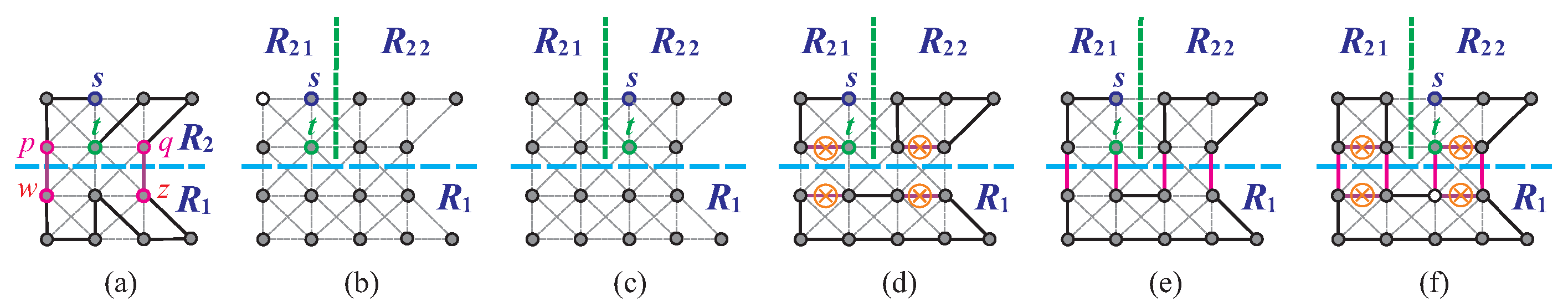
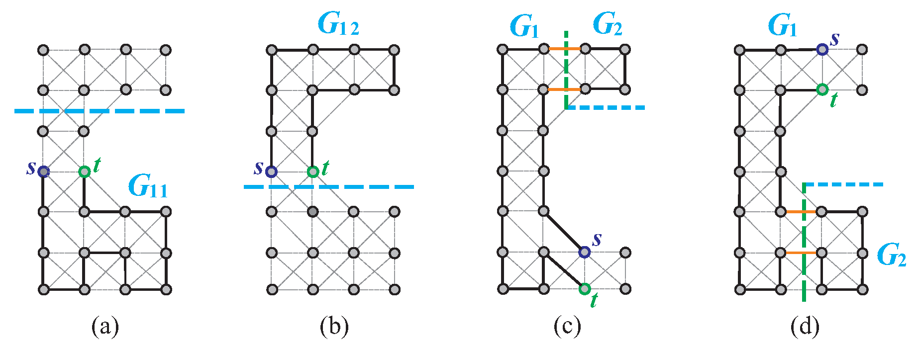
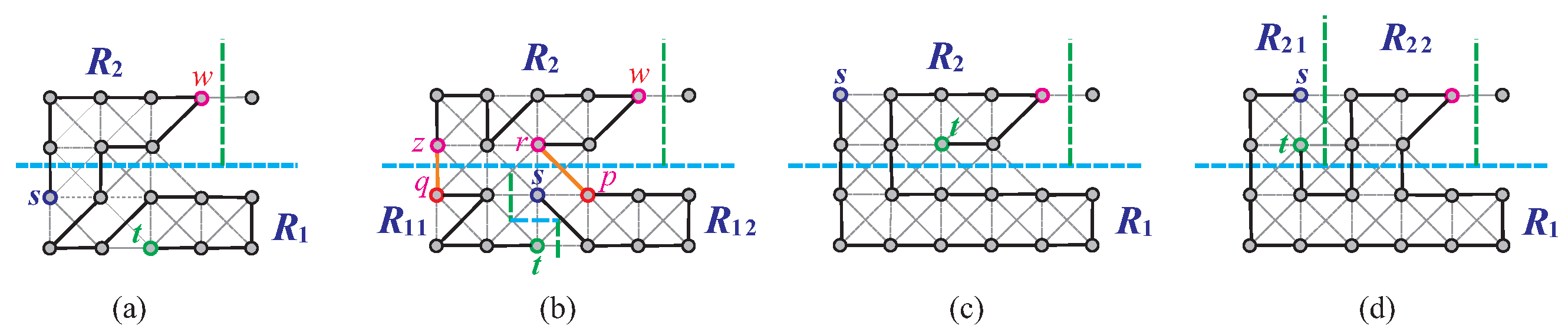
Case 6: Condition (UB12) holds. By Lemma 13, $\widehat{U}(C(m,n;k,l;c,d),s,t)=\widehat{L}(G_1,s,t)+1$, where $G_1=L(m,n;k,l+c)$. We make a vertical and a horizontal separation on $C(m,n;k,l;c,d)$ to obtain two disjoint supergrid subgraphs $R_2=L(n_2,m_2;1,1)$ and $R_1=R(m,n-n_2)$, where $n_2=c+l$ and $m_2=a+1$ (see Figure 27a). Note that $\left(C\right(m,n;k,l;c,d),$$s,t)$ does not satisfy condition (F1) in this case. Depending on the positions of s and t, these are the following three subcases:

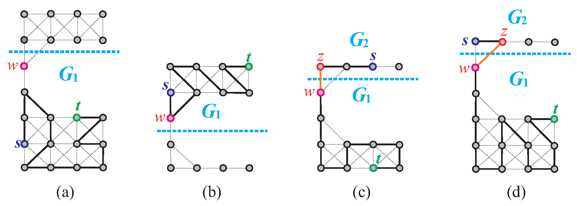
  Case 6.1: $s,t\in R_1$. A longest $(s,t)$-path of $\left(C\right(m,n;k,l;c,d)$ can be constructed by similar arguments in proving Case 1 of Lemma 10 (see Figure 27a,b). Then, we can construct a Hamiltonian $(s,t)$-path of $R_1\cup R_2$. Figure 27a,b depicts such constructions. The size of constructed Hamiltonian $(s,t)$-path equals to $\widehat{L}\left(L(m,n;k,l+c)\right)+1=\left|V(R_1\cup R_2)\right|$, and hence it is the longest $(s,t)$-path of $\left(C\right(m,n;k,l;c,d)$.

  Case 6.2: $s,t\in R_2$. A longest $(s,t)$-path of $\left(C\right(m,n;k,l;c,d)$ can be constructed by similar arguments in proving Case 2 of Lemma 10 (see Figure 27c,d). Depending on whether $\{s,t\}$ is a vertex cut of $R_2$, we consider Figure 27c,d. Then, we can construct a Hamiltonian $(s,t)$-path of $R_1\cup R_2$, as shown in Figure 27a,b. The size of constructed Hamiltonian $(s,t)$-path equals to $\widehat{L}\left(L(m,n;k,l+c)\right)+1=\left|V(R_1\cup R_2)\right|$, and hence it is the longest $(s,t)$-path of $\left(C\right(m,n;k,l;c,d)$.

  Case 6.3: $(s\in R_1$ and $t\in R_2)$ or $(s\in R_2$ and $t\in R_1)$. Without loos of generality, assume that $s\in R_1$ and $t\in R_2$. A longest $(s,t)$-path of $\left(C\right(m,n;k,l;c,d)$ can be constructed by similar arguments in proving Case 2.2 of Lemma 9 and Case 3 of Lemma 10.    □

Based on Lemmas 8–10 and Lemmas 11–14, we present Algorithm 1 to solve the longest path problem on C-shaped supergrid graph. Let the input of Algorithm 1 be a C-shaped supergrid $C(m,n;k,l;c,d)$ and vertices $s,t\in V\left(C\right(m,n;k,l;c,d\left)\right)$. In Algorithm 1, it needs to determine whether $\left(C\right(m,n;k,l;c,d),s,t)$ satisfies conditions (F1), (F3), (F7), (F8), or (F9). Clearly, it can be done in constant time. By Lemmas 8–10, $HP\left(C\right(m,n;k,l;c,d),s,t)$ does exist if $\left(C\right(m,n;k,l;c,d),s,t)$ does not satisfy any of conditions (F1), (F3), (F7), (F8), and (F9). By the proofs of Lemmas 8–10, $HP\left(C\right(m,n;k,l;c,d),s,t)$ can be constructed in $O\left(\right|V\left(C\right(m,n;k,l;c,d\left)\right)\left|\right)=O(mn-kl)=O\left(mn\right)$ time. Consider that $\left(C\right(m,n;k,l;c,d),s,t)$ satisfies conditions (F1), (F3), (F7), (F8), or (F9). By Theorem 5, $HP\left(C\right(m,n;k,l;c,d),s,t)$ does not exist. By the proofs of Lemmas 11–14, the longest $(s,t)$-path can be constructed in $O\left(\right|V\left(C\right(m,n;k,l;c,d\left)\right)\left|\right)=O(mn-kl)=O\left(mn\right)$ time. Thus, Algorithm 1 runs in $O\left(mn\right)$-linear time. We finally conclude the following main result.

Algorithm 1: The longest $(s,t)$-path algorithm.

Input: A C-shaped supergrid graph $C(m,n;k,l;c,d)$ with $mn⩾2$, and two distinct vertices s and t in $C(m,n;k,l;c,d)$. Output: The longest $(s,t)$-path. if$a(=m-k)=1$ and $\left(C\right(m,n;k,l;c,d),s,t)$ does not satisfy the forbidden conditions (F1), (F3), (F7), (F8), and (F9), then output $HP\left(C\right(m,n;k,l;c,d),s,t)$ constructed from Lemma 8; if$a(=m-k)>1$, $c=d=1$, and $\left(C\right(m,n;k,l;c,d),s,t)$ does not satisfy the forbidden conditions (F1), (F3), (F7), and (F8), then output $HP\left(C\right(m,n;k,l;c,d),s,t)$ constructed from Lemma 9; if$a(=m-k)>1$, $[c>1$ or $d>1]$, and $\left(C\right(m,n;k,l;c,d),s,t)$ does not satisfy the forbidden conditions (F1), (F3), (F7), and (F8), then output $HP\left(C\right(m,n;k,l;c,d),s,t)$ constructed from Lemma 10; if$\left(C\right(m,n;k,l;c,d),s,t)$ satisfies one of the forbidden conditions (F1), (F3), (F7), (F8), and (F9), then output the longest $(s,t)$-path based on Lemma 14.

Theorem 6.

Given a C-shaped supergrid graph $C(m,n;k,l;c,d)$ and its two distinct vertices s and t, Algorithm 1 computes a longest $(s,t)$-path in $O\left(mn\right)$-linear time.

Let G be a graph and let $\eta =\left|V\right(G\left)\right|$. The all-pairs longest path problem is to find the longest paths between all pairs of vertices in G. The most obvious solution to the all-pairs longest path problem is to run a longest path algorithm ${\eta }^2$ times since there are $\left(\genfrac{}{}{0pt}{}{\eta }{2}\right)=\frac{\eta (\eta -1)}{2}$ pairs of vertices. Let $G=C(m,n;k,l;c,d)$. Then, $\eta =mn-kl=O\left(mn\right)$. By calling Algorithm 1 ${\eta }^2$ times, the all-pairs longest path problem for $C(m,n;k,l;c,d)$ can be solved. Thus, the following corollary holds true.

Corollary 1.

Given a C-shaped supergrid graph $C(m,n;k,l;c,d)$, the all-pairs longest path problem can be solved in $O\left(m^3{n}^3\right)$ time by calling Algorithm 1 ${(mn-kl)}^2$ times.

5. Conclusions

The Hamiltonian problems can be applied to many fields including computer science, biology, molecular science, etc. However, they are NP-complete for general graphs and supergrid graphs. The Hamiltonian path problem is a special case of the longest path problem, and hence the longest path problem is generally difficult. The time complexities of these problems for solid supergrid graphs are still unknown. In this paper, we study these problems on C-shaped supergrid graphs, which form a subclass of solid supergrid graphs. We first discover some Hamiltonian connected properties of rectangular supergrid graphs. We then prove C-shaped supergrid graphs to be Hamiltonian connected except in a few conditions. Finally, we presented a linear-time algorithm for finding a longest path in C-shaped supergrid graphs between any two given vertices. This result can be applied to find the longest path on C-like objects with a supergrid structure. It is well known that Floyd’s algorithm computes all-pairs shortest paths of a digraph. It is interesting to construct a modification of Floyd’s algorithm for solving the all-pairs longest path problem on C-shaped supergrid graphs in linear time. We will post it as an open problem for interested readers. In addition, Laplacian matrix is a matrix representation of a graph. Together with Kirchhoff’s theorem, it can be used to calculate the number of spanning trees for a given graph. It is interesting to see whether there exists a modification of the above result such that it can compute the number of longest paths between two vertices in C-shaped supergrid graphs efficiently. We would like to post it as an open problem to interested readers.