1. Introduction
Increasing competition and the associated intensification of global business are characteristic factors for modern manufacturing companies. Other factors, such as the ongoing digital transformation and a growing demand for customized products have to be considered as well. An economically optimal utilization of the production chains was often considered as the essential goal in the past. During the last years, however, this goal has increasingly shifted towards a more customer-oriented production. Accordingly, the focus of all companies is now on the time feasibility and adherence to promised delivery dates, which confronts operational production planning with questions about the latest possible release of a certain batch, so that it can still be manufactured and delivered on time. A constantly increasing complexity of production systems, in conjunction with a high degree of automation, repeatedly poses challenges for many production companies. As a result, there is an increasing need to use optimization algorithms in practice in order to handle the complexity of planning problems. This is especially the case in the use case of this study, which comes from the field of semiconductor manufacturing. The use of simulation-optimization approaches [
1] could provide a differentiated answer. In planning, design, and ramp-up, these methods are well established but are not frequently used yet for operational support in decision-making.
In our real-life scheduling application, and other production use cases, it is possible for jobs to take different paths through the production system. The specific path might depend upon a particular specification or parameter, which defines the machines to be visited by the job. The existence of different paths through the production system might cause time dependencies, so the order in which the jobs leave the system might be different from the order in which the jobs entered it. Consequently, this can lead to problems in the context of the planning of batch-related insertion dates, especially if batch processes are also found within the production system. Therefore, we need a simulation to model our system. In this study, a multi-path version of the hybrid flow shop scheduling problem [
2] was analyzed. This version also considers two batch processes at the same time, and it is based on the real case from a German manufacturing industrial partner. Furthermore, a global priority rule and a “same setup” rule were considered. The before-mentioned elements make the computation of the makespan a non-trivial task: due to the existence of time-dependencies and batches, the makespan cannot be computed using a closed analytical expression anymore.
Accordingly, the main contributions of this study are described next: (i) a simulation model of a hybrid flow shop problem with pre-determined paths, which are predefined by individual parameters and specifications and batching; (ii) a fast discrete-event heuristic that is able to deal with the complexity of the modeled system and compute the makespan associated with a proposed solution; (iii) the extension of the previous heuristic to a biased-randomized algorithm [
3], which introduces some degree of randomness into the heuristic constructive process; and (iv) the evaluation of computational experiments, which show the performance of the proposed methodology for solving this scheduling problem. Concepts of discrete-event simulation and heuristic algorithms can be combined into discrete-event driven heuristics. Some typical applications include scenarios in which synchronization issues are relevant [
4] or in which rare events have to be modeled [
5,
6]. Furthermore, biased-randomized algorithms may generate alternative solutions based on heuristic dispatching rules. By making use of Monte Carlo simulation and skewed probability distributions, biased-randomized techniques introduce a non-uniform random behavior into a dispatching rule. Employing parallelization techniques, these heuristics can be applied in the same computational time as the original dispatching rule, thus making these algorithms much more powerful than the original heuristics they build upon. In the literature, applications of these algorithms can be found in flow shop problems [
7]. Despite its importance in the semiconductor industry, to the best of our knowledge, a flow shop problem such as the one described here has never been solved in the related literature.
The article is organized as follows.
Section 2 provides a more-detailed description of the scheduling problem studied in this article.
Section 3 reviews related work on similar flow shop problems.
Section 4 describes the algorithms proposed in this work in as much detail as possible, so they can be reproduced by other researchers or practitioners.
Section 5 carries out a series of numerical experiments to test our methodology and analyzes the obtained results. Finally,
Section 6 summarizes the main findings of this study and points out some future research lines.
2. A Detailed Description of the Problem
This section describes a hybrid flow shop problem with realistic constraints. The example described here is based on the specifics and constraints of a pre-assembly process in semiconductor manufacturing, and notice that these constraints commonly appear in semiconductor manufacturing in general.
In parallel with the realistic use case, in this section, we formally categorize our problem. Therefore, we use the notation first introduced by [
8]. Using the scheme, any scheduling problem can be described by means of a parameter tuple
[
9]. The parameter
defines the number, the type, and the arrangement of the machines and stages. The second parameter,
, can contain any number of entries. The entries are separated by commas.
represents characteristic features and restrictions of the production process. The last expression,
, within the tuple stands for the objective function. Single objective functions, combinations of objective functions in a mathematical expression, or different tested objective functions can be specified here [
9].
Due to production systems getting more complex and specified during the time, Graham’s notation [
8] was further specified by [
9,
10] with additional production environments (
), constraints (
), and objectives (
). In this section, elements of their notations are also utilized to characterize our problem. Further, we explain the specifics of the use case and characterize the components of the problem by Graham’s notation in brackets.
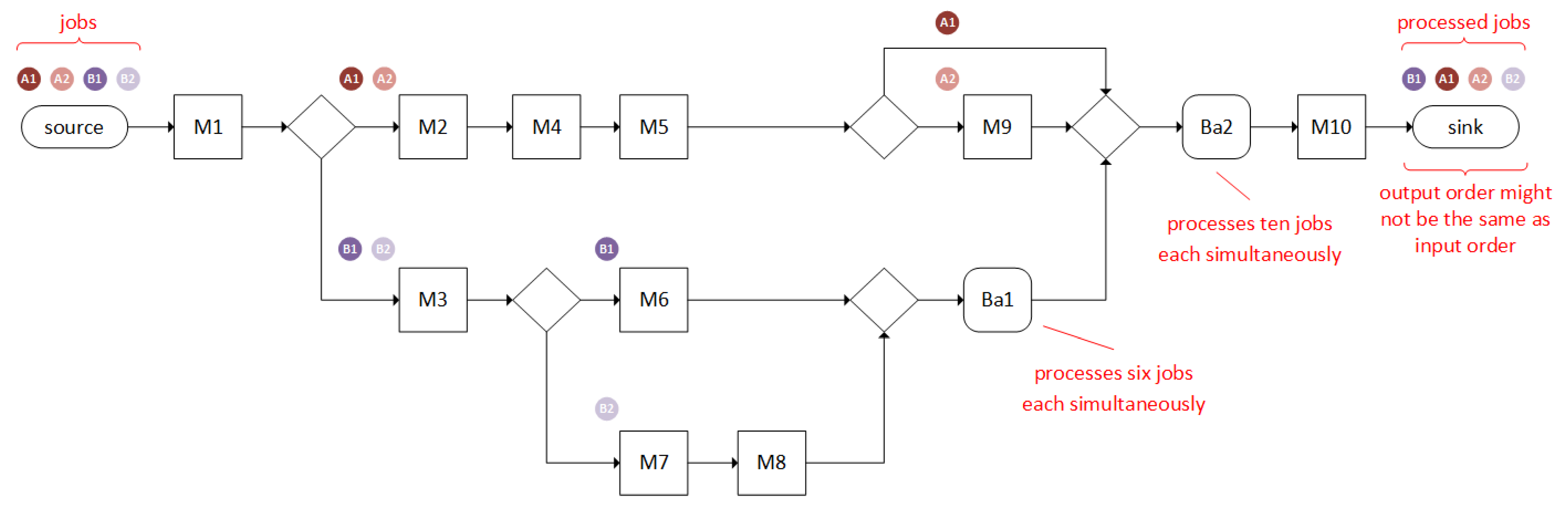
Figure 1 shows the problem we are considering. The production contains 10 machines and 2 batch processes. Flow shops with multiple machines on one of the processing stages are referred to as hybrid or flexible flow shops (
) [
9,
10]. Hybrid flow shop environments with machines that need different types (or a specified amount) of jobs to start their production can be categorized as assembly flow shops [
11,
12]. In contrast, hybrid flow shops with machines that may process jobs of different types simultaneously (see machine
and
in
Figure 1) are referred to as
with batching machines (
) [
9,
13].
The described machines
process jobs
of different product types
or families (in Graham’s notation known as
) [
9], where
. The four possible product types
are
. Depending on the product type, the jobs are processed along a specific route, which consists in a defined sequence of machines.
While the jobs j are all processed on machine M1 after being loaded into the modeled system, the jobs j are subsequently divided into different paths depending on their product types . On the one hand, jobs of product types are processed by machines , , and , while jobs of product type are processed on machine . Jobs of product types and () are not processed on machine but on machine and, subsequently, by machine in the case of product type . In the case of product type , they are processed by machines and . Our model includes machine qualifications (). In contrast, for example, jobs of type skip machine . Accordingly, the model contains the constraint of skipping stages (). According to a load of jobs with different product types—and thus different processing sequences—it is possible that jobs are processed at different speeds through the flow production scenario.
In general, a global-priority-rule procedure applies to the modeled system. Accordingly, the orders of product type are prioritized, i.e., orders (if available) are always given priority on a machine (). In addition, a “same setup” priority rule applies to the entire flow production scenario (apart from the batch processes). This rule sorts the jobs in the queue depending on the setup status of the machines in order to keep setup times and their influence on the makespan to a minimum. These constraints are based on a “real-world use-case” from the field of semiconductor manufacturing and are depicted in a simplified form in this model. Accordingly, in semiconductor manufacturing, countless product types are often fed into the system, which requires a special setup on the machines. In order to shorten the setup times and subsequently the overall makespan of the jobs, jobs of the same product type are given priority if possible (same setup). The prioritization of a specific product type (in this case, product type ) is also used to prioritize product types with a high order volume, high makespans, and/or complex setups.
Unlike other machines, the machines
process several jobs
j simultaneously. Hence, they are referred to as batch machines, whereby the product types are negligible. Accordingly, six jobs
j are processed simultaneously on machine
. The processing of the job
j begins as soon as a total of six jobs of product types
and
are waiting in the machine. The ratio of jobs
j of product type
or product type
is irrelevant. On machine
, a total of ten jobs is processed simultaneously, whereby these can be jobs of product types
,
,
, and
[
13].
The objective of the study was to find a permutation of jobs (solution) that reduces the makespan
(which is the last component of Graham’s notation). In Graham’s notation [
8], which was extend by [
9,
10], this problem can be completely formalized as:
3. Related Work
Flow shop problems have been studied since the early 1950s [
14]. Several authors have employed mixed-integer programming, heuristics, and discrete-event simulation to deal with hybrid flow shops in different application areas [
13,
15,
16]. The flow shop problem is NP-hard even for a problem with two-states, two identical parallel machines on one of both stages, and one machine on the other stage [
17]. Hence, the problem we analyzed in this study is classified as NP-hard. In contrast to exact optimization methods, heuristics cannot verify the optimality of a solution. However, they can provide high-quality (or even near-optimal) solutions in short computational times, something that cannot be generally achieved with exact methods [
18,
19].
Several reviews on assembly flow shops can be found in the literature [
11,
12]. A review of hybrid flow shops with the integration of batching components is provided in [
13]. As stated by some authors, the makespan and time-based objectives dominate the literature in flow shop environments [
11,
15]. Hence, the makespan is one of the most relevant objectives both in theoretical as well as in applied works.
In the hybrid flow shop literature, two possible expressions of priority sets can be observed. First, there is a fixed defined ranking of priority groups such as
,
,
. Secondly, for each job
j, a set of preceding jobs
is defined [
20].
Some studies consider hybrid flow shop problems with batching machines, priority rules, and makespan objectives [
20]. In the aforementioned work, a complex and realistic flow shop problem with changeover times, machine qualifications, and priority rules was analyzed. To deal with this problem, the authors have extended the NEH [
21] considering machine qualification, skipping stages, and rule priorities. The authors concluded that the NEH heuristic provides good results for this type of flow shop problem.
Additionally, for the hybrid flow shop problem with setup times, machine qualifications, delayed machine availability, lag times between the stages, and the makespan objective, other authors compared the priority rules of the “shortest processing time,” the NEH, and the “longest processing time”, concluding that the NEH offers the best results [
22]. A genetic algorithm for a hybrid flow shop with batching machines was introduced in [
23]. In addition, the latter work allows jobs to skip stages. The initial solution for the genetic algorithm was generated by a “longest processing time” dispatching rule, followed by the “earliest completion time” heuristic for the following stages. A tabu search has also been proposed for a hybrid flow shop in [
24]. This algorithm swaps two jobs in each iteration. The tabu list tracks pairs of jobs that were swapped in previous iterations to avoid loops. Three dispatching rules were compared for generating the initial solution: two variations of the “longest processing time,” with the sum of the processing times over all stages per order, and an alphanumeric ordering. As a result, the authors showed that none of these strategies performs significantly better than the other.
A “shortest processing time” heuristic for a two-stage hybrid flow shop problem with polynomial runtime was introduced in [
25]. Here, jobs can only be processed by one dedicated machine on stage one. In the following stages, all jobs are processed on one machine in the batch processing mode. The “shortest processing time” heuristic was employed for allocating the jobs on the first stage, and a combination of the “earliest completion time” and a minimization of the processing times for all batches was employed on the second stage. Due to the high complexity of the problem considered in our study, a large number of possible permutations need to be explored. As mentioned before, simulation can be useful for modeling, but it needs to be combined with optimization components in order to generate high-quality or even near-optimal solutions.
4. A Biased-Randomized Discrete-Event Algorithm
In order to solve the hybrid flow-shop problem with batch processes, setup times, and priorities, a multi-start approach is proposed in Algorithm 1. This multi-start method calls a biased-randomized heuristic (Algorithm 2) that makes use of the NEH heuristic. As discussed above, variations of this heuristic can provide good results for many hybrid flow shops [
6]. The original NEH was designed to minimize the makespan in a simple flow shop environment.
Due to the complexity of the flow shop system considered in this work, we made use of an original discrete-event based heuristic to compute the makespan. This procedure is outlined in Algorithm 3. Our approach, which is depicted in Algorithm 1, receives as input parameters a job list
(where
is the job situated in the
position in the sequence), some parameters
, and the
parameter (
) of the geometric distribution employed to induce the biased-randomization effect [
26]. This algorithm works as follows: firstly, the initial solution
is generated by means of the heuristic STNEH (
) at line 2. In the main loop, the algorithm iterates until the termination criterion is not reached. For each iteration, a new solution
is generated by using the biased-randomized version of the STNEH heuristic, BR-STNEH. This is achieved by setting
in the interval
, as explained in [
27]. If the makespan of
is lower than solution
, then
is replaced by
; otherwise
is discarded.
Concerning the biased-randomized algorithm BR-STNEH (Algorithm 2), it chooses in each iteration the next job according to a two-level criterion: the setup times in the first level and the processing times in the second-level. Consider the following parameters: the jobs list
, the
parameter, the job processing times
, job setup times
, a list of job types
, and a non-negative integer
. The algorithm starts by listing the job types
to split
into a list of jobs of type
called
. The NEH heuristic is applied to each list
and collected in a list of lists
(lines 3–7). In line 8,
is sorted in descending order according to setup times. This is done because the setup time occurs mainly when two jobs, of different types, are processed by the same machine consecutively. Hence, if we classify the jobs by type, and then sort by the setup time
, we can expect a reduction in the number of times that two jobs of different types are processed by the same machine. In lines 9–12, those jobs that are a priority (
) must be scheduled at the beginning of the
. The main loop iterates until all jobs are scheduled. For each iteration, the algorithm picks a type
from
list and gets randomly an integer number
between 1 and
, i.e., the latter fixes the number of iterations of the inner loop. In the inner loop, a random job is selected from the list
and appended to the partial solution in each turn (lines 16–21). Finally, the complete solution
is returned. This procedure is then extended into a biased-randomized algorithm by introducing the geometric distribution
with parameter
.
| Algorithm 1 Multi-Start Framework |
- 1:
Multi-Start(, , ) - 2:
←BR-STNEH(,, ) - 3:
while end criteria not reached do - 4:
←BR-STNEH(, , ) - 5:
if makespan(,) <makespan(,) then - 6:
← - 7:
end if - 8:
end while - 9:
return best
|
| Algorithm 2 Biased Randomized STNEH |
- 1:
BR-STNEH(, , , , , ) - 2:
- 3:
for alltypeJob ϵ types(jobsList) do - 4:
- 5:
SortingByNEH(, ) - 6:
append(,) - 7:
end for - 8:
SortingBySetupTimes(,) - 9:
for alltypeJob ϵ typesPriority do - 10:
extend(,) - 11:
remove(,) - 12:
end for - 13:
while is not complete do - 14:
pickList(,) - 15:
← randomInt(1,) - 16:
while do - 17:
pickJob(,) - 18:
append(,) - 19:
remove(,) - 20:
- 21:
end while - 22:
if then - 23:
remove(,) - 24:
end if - 25:
end while - 26:
return
|
In order to compute the makespan, we developed a discrete-event based procedure. The idea of this methodology is to use a discrete-event list to manage complex time dependencies that arise as events occur over time [
4]. This event list is constantly sorted, taking into account the chronological order of each event (e.g., the assignment of a job to an available machine or the arrival of a job to a batch queue), and it is iteratively processed until no events are left. Making all decisions in chronological order avoids complex and time-consuming back-rolling issues. Hence, when a new event is scheduled, it is chronologically inserted into a list
. The makespan is iteratively computed as this
is processed, and others are scheduled, following a chronological order. Algorithm 3 shows an overview of the proposed discrete-event procedure. The algorithm receives as input parameters the
, which is the complete list of jobs in the specific order that will enter in the system to be processed the machine-dependent processing times of each job (
) and the setup times of each job-machine (
). The algorithm requires auxiliary data structures, such as:
(i.e., at which time a machine
m will be available),
(which keeps track of the machine that previously processed the job),
(which stands for the type
that machine
m can process), and
(which stores a set of jobs in the batch
m). In the beginning, all jobs are being processed in machine 1, in concordance with the scheduling
. Therefore, the algorithm is initialized, creating ending events at machine 1 and inserting them into the event list
(lines 9 to 16). In line 17,
is sorted by time
t of occurrence. The main loop iterates until
is empty.
| Algorithm 3 Discrete-Event Makespan Method |
- 1:
makespam(,,) - 2:
initAvailableTimes() - 3:
initPreviousTypeMachine() - 4:
initMachinesType() - 5:
initJobsWaiting() - 6:
emptyList - 7:
- 8:
for alljob ϵ jobList do - 9:
- 10:
if then - 11:
- 12:
end if - 13:
- 14:
createEndingEvent(t,,) - 15:
append(,) - 16:
end for - 17:
sortingByTime() - 18:
whiledo - 19:
first() - 20:
if isStarting() then - 21:
processingStartingEvent(, , , , , ,) - 22:
else - 23:
processingEndingEvent(, , , , , , ,) - 24:
end if - 25:
time() - 26:
end while - 27:
return
|
At each iteration, the next event, , is selected, which can belong to one of the following types: job starts in a machine (starting-event) or job ends in a machine (ending-event):
In case of a starting-event, job is just placed at the entrance of machine j at time t. Algorithm 4) proceed as follows: job , machine , time t, and type are recovered in lines 2–4; in line 6, we check whether belongs to the path; if it does not, then a new ending-event is created with the same job, machine, and time (lines 18–19); otherwise, the algorithm advances the clock time t; next, the algorithm determines the , which is set to 0 if the previous job type and the current one match; otherwise, ; hence, the new time is set to previous time t plus the job-processing time and the (lines 7–14); finally, we create a new ending-event with the same job and machine but at time ; this event is insert into the event list.
| Algorithm 4 Processing Starting Events |
- 1:
processingStartingEvent(, , , , , ,) - 2:
job() - 3:
type() - 4:
machine() - 5:
time() - 6:
ifthen - 7:
- 8:
- 9:
if then - 10:
- 11:
end if - 12:
- 13:
- 14:
- 15:
createEndingEvent(,,) - 16:
insertEventSorted(,) - 17:
else - 18:
createStartingEvent(t,,) - 19:
insertEventSorted(,) - 20:
end if
|
In case of an ending-event (Algorithm 5), like a job of type leaving machine at time t, the algorithm works as follows: initially, job, type, and time are obtained from event in lines 2–3; in line 4, this machine release time is computed with the maximum between the current time t and the current machine release time ; then, the algorithm verifies whether the job belongs to this machine path; if it does not, then a new starting-event is created with the same job and time but in the next machine (lines 18–19); otherwise, it continues to the next step; in the next step, our algorithm assumes that the size of all batches is set to 1 except for and ; hence, the current job is added to the list of jobs in the current machine (lines 8–9); in lines 10–16, the algorithm checks if the number of jobs in this machine reaches the batch size, in which case a new starting event is scheduled at time t for each job in the (these new events are inserted into the ).
Finally, when
is empty (line 18 in Algorithm 3, the algorithm finishes returning the time
of the last event processed, which is an ending-event of the last job in the last machine. This time is the makespan of the processed
.
| Algorithm 5 Processing Ending Events |
- 1:
processingEndingEvent(, , , , , , ,) - 2:
job() - 3:
type() - 4:
machine() - 5:
time() - 6:
- 7:
ifthen - 8:
- 9:
add(,) - 10:
if then - 11:
- 12:
for do - 13:
createStartingEvent(t,,nextMachine()) - 14:
insertEventSorted(,) - 15:
end for - 16:
end if - 17:
else - 18:
createStartingEvent(t,,nextMachine()) - 19:
insertEventSorted(,) - 20:
end if
|
5. Computational Experiments
The proposed algorithm was implemented using Python
. All experiments were run in a computer with an Intel Xeon E5-2650 v4 with 32GB of RAM. As far as we know, there are no public instances for the studied problem. Hence, we generated a set of instances, which are available at
https://www.researchgate.net/publication/356874077_instances_flowShop (access on 1 February 2022). This set consists of 20 instances, and it is based on the production scenario defined in
Section 2, which includes ten processing machines and two additional batch machines, distributed in four different paths. A total of four different types of jobs were considered, each type being processed on a specific path. The instances were identified following the nomenclature
, where
j is the sum of jobs to be processed;
m defines the sum of machines (including both regular and batching machines); and
y is a sequential number, used to identify the instances with the same number of jobs and machines in an easy and comprehensive way. Notice that, depending on the instance, the number of jobs varies between 30 and 1600. We defined unrelated and machine-dependent setup times for every job. Thus, every job has different set-up times on every machine. We also defined unrelated and machine-dependent processing times. Hence, for each job
j, a processing time at each machine
i was defined. Our algorithms were run considering 60 s of computing time for instances with 30 jobs and 300 s for instances with 200 and 400 jobs, while it employed a maximum of 900 s for instances with 800 jobs or more.
Table 1 shows the results of the algorithm described in
Section 4 for the defined instances. The first column identifies the instance. Subsequently, the following two columns present the solutions obtained using the AnyLogic simulation tool, which simulates the production scenario. In that sense, we provided the total makespan of each solution when the jobs are processed in the system using a first-in-first-out (FIFO) strategy and the computation time—in seconds—required to reach them. Using this strategy, the jobs enter in the system without any logical ordering, i.e., following the alphanumerical order as provided in the instances. We provide this information with the aim of validating the quality of our algorithm. Similarly, the next two columns report the makespan, with its corresponding computational time, provided by our approach using the above-mentioned FIFO strategy. The following two columns present the results of our approach using the same strategy combined with biased-randomization techniques. This allows us to enter jobs in the system in a different order at each algorithm iteration. In our case, a geometric probability distribution, driven by a single parameter
was employed to induce this behavior. The value for this parameter was set after a quick tuning process over a random sample of instances, establishing a good performance whenever
falls between
and
(i.e., any random value inside this interval will generate similar results). Specifically, these columns provides the best-found solution (makespan) and the computational time—in seconds—to reach it. Similarly, the next four columns display the makespans and the computational times when the BR-NEH and BR-STNEH sorting strategies were applied. Finally, the last three columns of the table report the gaps for the different strategies with respect to the initial FIFO one.
Our results show that our approach is highly competitive regarding computational times with respect to the Anylogic simulator. Notice that for large instances (e.g., 1600 jobs), our approach provides solutions in times less than
s using the FIFO deterministic strategy, while Anylogic requires times greater than five seconds of computation to provide the same solutions. Regarding the different sorting methods,
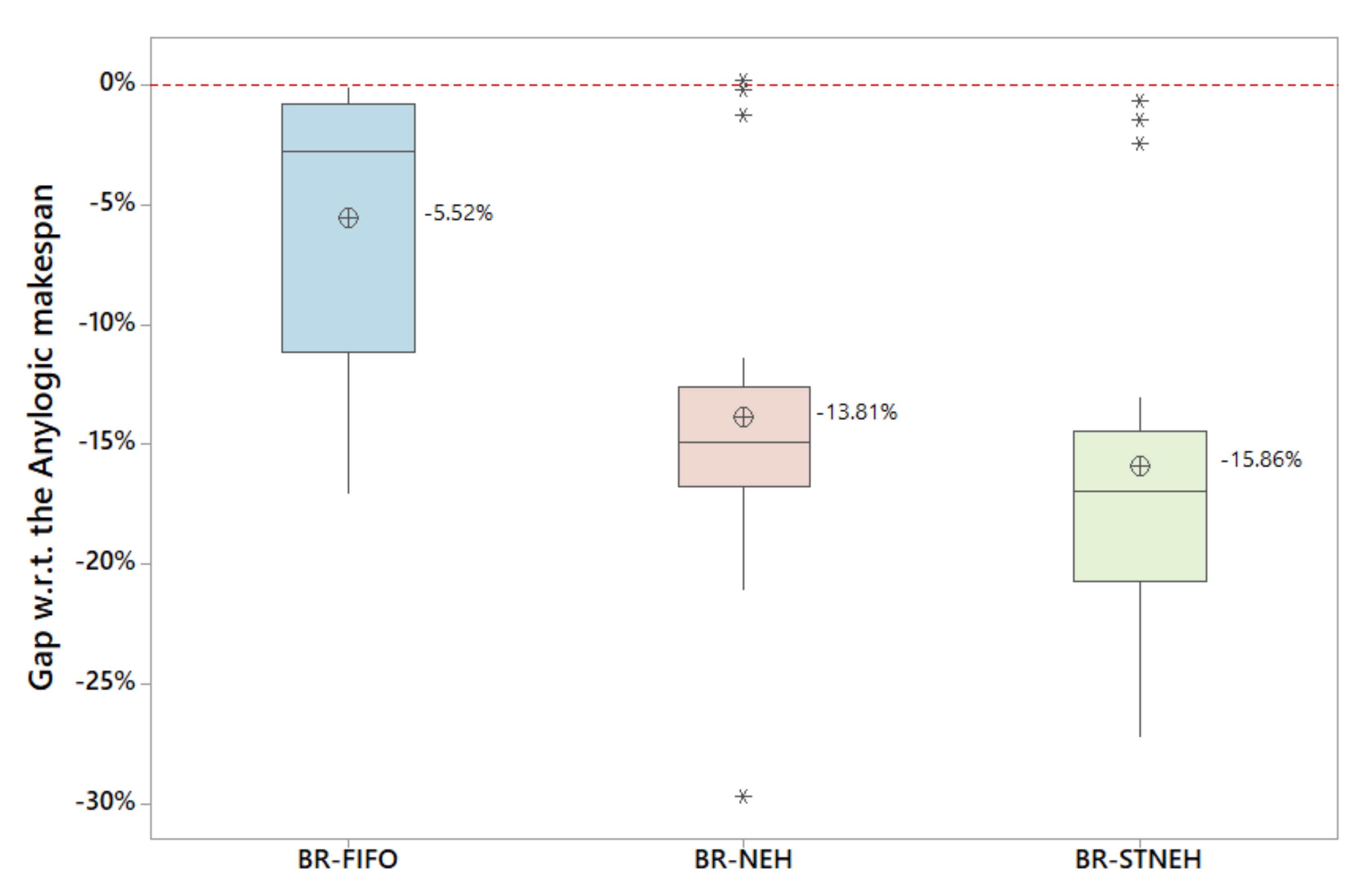
Figure 2 summarizes the results provided in
Table 1, where the vertical axis of the boxplot represents the gap obtained with respect to the FIFO strategy. Notice also that, after applying biased-randomized techniques on the original FIFO strategy, the average gap outperformed the former by about
% on the average. The original FIFO strategy does not contain any optimization strategy, it just dispatches jobs in the original order. Hence, improvements are achieved as more-intelligent sorting methods are used to dispatch the jobs. In that sense, the BR-NEH sorting method, which is based on sorting the jobs by total processing time in decreasing order, is able to enhance the original heuristic by
on average. Notice that the setup times of each job–machine pair may induct to lose the logic behavior of the NEH heuristic, since jobs with short processing times and large setup times are not prioritized in the sorted list of jobs. Thus, to address this limitation, the BR-STNEH sorting method also considers the setup times of each job-machine pair during the sorting process, outperforming the BR-NEH by about
(obtaining an average gap of
with respect to the initial FIFO strategy). Regarding the computational times, on average, there were no significant differences between the BR-NEH and BR-STNEH sorting methods to reach the best-found solution.
6. Conclusions
This study considered a hybrid flow shop problem with time dependencies, batching requirements, and priority rules. The model analyzed is based on a real-life system in the semiconductor industry. Due to the existence of time dependencies, it is not possible to compute the makespan associated with a proposed solution by simply using a analytical expression, and a simulation needs to be carried out each time a new solution is provided. Apart from being time-consuming, using a pure simulation does not allow us to generate high-quality solutions, in general. In order to solve this problem, a fast discrete-event-based heuristic was proposed. This heuristic is capable of proposing a promising solution—one based on a certain constructive logic—while, at the same time, it computes its associated makespan. Moreover, the heuristic is extended into a full probabilistic algorithm by incorporating biased-randomization techniques. Hence, making use of a skewed probability distribution (a geometric one in our case), our biased-randomized discrete-event algorithm is capable of generating high-quality solutions in fast computational times, thus easily outperforming the ones provided by a state-of-the-art simulation software.
Several research lines can be considered for future work, among them: (i) the “longest processing time first” or other priority rules can be used as a basic procedure for the biased-randomized discrete-event algorithm and (ii) our approach could be extended into a full simheuristic [
28] to account for scenarios where processing times have a stochastic nature.


 ,
, 

