Convex Neural Networks Based Reinforcement Learning for Load Frequency Control under Denial of Service Attacks

Abstract

With the increase in the complexity and informatization of power grids, new challenges, such as access to a large number of distributed energy sources and cyber attacks on power grid control systems, are brought to load-frequency control. As load-frequency control methods, both aggregated distributed energy sources (ADES) and artificial intelligence techniques provide flexible solution strategies to mitigate the frequency deviation of power grids. This paper proposes a load-frequency control strategy of ADES-based reinforcement learning under the consideration of reducing the impact of denial of service (DoS) attacks. Reinforcement learning is used to evaluate the pros and cons of the proposed frequency control strategy. The entire evaluation process is realized by the approximation of convex neural networks. Convex neural networks are used to convert the nonlinear optimization problems of reinforcement learning for long-term performance into the corresponding convex optimization problems. Thus, the local optimum is avoided, the optimization process of the strategy utility function is accelerated, and the response ability of controllers is improved. The stability of power grids and the convergence of convex neural networks under the proposed frequency control strategy are studied by constructing Lyapunov functions to obtain the sufficient conditions for the steady states of ADES and the weight convergence of actor–critic networks. The article uses the IEEE14, IEEE57, and IEEE118 bus testing systems to verify the proposed strategy. Our experimental results confirm that the proposed frequency control strategy can effectively reduce the frequency deviation of power grids under DoS attacks.

1. Introduction

With the rapid economic growth, the increase in electricity demand and the large-scale access of distributed energy sources have made the scale of power grids increasingly large and complex, thereby, introducing more power grid disturbance factors. Power grid disturbances (such as load change disturbances, etc.) may degrade the power quality of the frequency and threaten the security of power grids [1,2,3], and thus it is necessary to impose load-frequency control on power grids to maintain the power frequency on a fixed value (e.g., 50 and 60 Hz).

Load frequency control, as a means to maintain the balance of supply and demand, is re-emphasized when a large number of distributed energy sources are connected. Aggregated distributed energy sources (ADES) are connected to power grids based on fast-response power electronics and aggregated output techniques, which provides a new flexible implementation method for load-frequency control [4,5].

ADES can quickly respond to the control instructions issued by digital computers [6,7], eliminate frequency deviation, and stabilize the frequency in a relatively small range in the presence of interference. ADES consists of multiple small energy storage systems. Compared with a single energy storage system, ADES may have greater power and capacity ratings, and it can be regarded as an entity of system operation.

In this process, the ADES controller typically distributes the sub-control tasks to a single node. The ADES controller assigns the realization task of control output to each distributed energy system for realization. However, in this paper, this research focuses on the intelligent frequency modulation algorithm, and the dispatch method of the aggregator has been investigated in many studies [8,9,10,11]. Therefore, this paper does not give a detailed introduction to the dispatch algorithm.

At present, some methods have been proposed for the frequency control of power systems [12,13,14,15,16]. As a high-dimensional nonlinear complex large-scale system, the control strategy design of modern power grids (the control output of ADES controllers) involves large-scale analytical modeling [17,18,19]. Data-driven methods are often used to solve the analytical modeling issues [20,21].

Reinforcement-learning techniques as a type of data-driven method can effectively solve the frequency control issues of complex power grids [21]. Reinforcement learning aims to directly optimize the control strategy of power grids based on the measured frequency data without analyzing the influence of the accurate analytical model of power grids in the control process. With appropriate training and cost-return functions, data-driven frequency control methods based on reinforcement learning can achieve good control performance. Reinforcement learning can easily obtain a suitable power grid frequency control strategy under nonlinear working conditions [22].

Ahamed et al. [23] proposed an adaptive nonlinear control technique that applied reinforcement learning to the frequency control issues of single-region power grids. Z. Yan et al. proposed a deep reinforcement-learning (DRL) model in continuous scope to improve the load frequency performance of single-region power grids [22]. However, the concurrent learning of multi-zone controllers causes the overall operating environment to be no longer stable. Such learning algorithms lack consistent gradient signals in multi-region power grids [24]; therefore, they cannot guarantee frequency control performance in a cooperative manner.

A multi-agent reinforcement-learning (MARL)-based frequency control strategy was proposed to solve the frequency control issues in multi-region power grids with a co-current learning convergence guarantee [25,26]. This strategy divides each sub-region of multi-region power grids into a single agent. Each agent coordinates to control the frequency of multi-region power grids.

In addition to the challenges brought by the large-scale system modeling of power grids, the destructive impacts caused by cyber attacks have brought new challenges to the design of power grid control systems following the rapid advancement of power grid digitization and informatization [15]. Denial of service (DoS) attacks are common network attacks in information attacks. DoS attacks damage the integrity and timeliness of communication data by blocking communication channels [27,28].

In addition, these attacks also reduce the performance of power grid control systems and cause transient instability of power grid phase angles in severe cases or even system collapse. Thus far, there have been many power failures caused by DoS attacks [29,30].

Therefore, it is significant to conduct related research regarding power grid frequency control under DoS attacks. The existing research has proposed certain solutions for power system frequency control under network attacks, including resilient model predictive control [12], event triggering control [13], etc. The methods used to resist DoS attacks include data dimensionality reduction [31], data filtering [32], and event-triggered control structure [33]. In particular, actor–critic structure algorithms in reinforcement learning [34,35,36] can be used to defend against DoS attacks.

In actor–critic structure reinforcement-learning algorithms, the actor and critic play different functions. The actor is used to output control strategies. The critic is used to evaluate the rationality of the current control strategy formulated by the actor. Actor–critic structure algorithms focus on obtaining parameter vectors or network weights that can maximize the return by using the gradient descent update method.

Actor–critic structure algorithms can be implemented by neural networks, such as back-propagation neural networks (BPNN) [37] and radial basis neural networks (RBFNN) [38]. BPNN was used to implement both actor and critic networks in the actor–critic structure algorithms [34,35,36]. However, BPNN may cause the optimization process of reinforcement learning to only reach the local optimum during the implementation of critic structure, resulting in suboptimal control output [37,39].

The traditional model-based frequency control strategy cannot solve the problem of large-scale analytical modeling of control strategy in modern power systems. Although data-driven approaches (reinforcement learning etc.) have been proposed to solve this problem, the rapid response of control strategy optimization in reinforcement learning has not been well considered. There may be a local optimization problem of any control strategy.

Therefore, in order to improve the performance of load-frequency control under DoS attacks, this paper introduces convex neural networks [40,41,42,43] to realize the actor–critic structure. Convex neural networks are used to approximate the long-term goal of reinforcement learning and the output of the controller.

The optimization process of reinforcement learning is transformed into a convex optimization process. When partial weights of the convex neural networks meet certain constraints, the output of the convex neural networks is a convex function of the input. This ensures the existence of the global optimum and improves the efficiency of the optimization process. This paper has two main contributions as follows.

• In this paper, we propose a load-frequency control strategy of convex neural network-based reinforcement learning that can resist DoS attacks and analyze the sufficient conditions for the stability of power grids as well as the convergence of convex neural network parameters during online learning.
• A long-term utility model of load-frequency control based on convex neural network approximation is proposed. Thus, the control output can be improved by the near global optimum obtained from the convex approximation. Additionally, the optimization speed is accelerated, and the efficiency of controllers is improved.

The remainder of this paper is organized as follows. Section 2 introduces power grid models and DoS attack models. Section 3 describes the reinforcement-learning framework based on convex neural networks and the design and online learning of frequency controllers and derives sufficient conditions for the system stability and convergence of neural network weights. Section 4 simulates the proposed algorithm in three IEEE bus testing systems to verify the effectiveness and advancement of the proposed strategy. Section 5 concludes this paper.

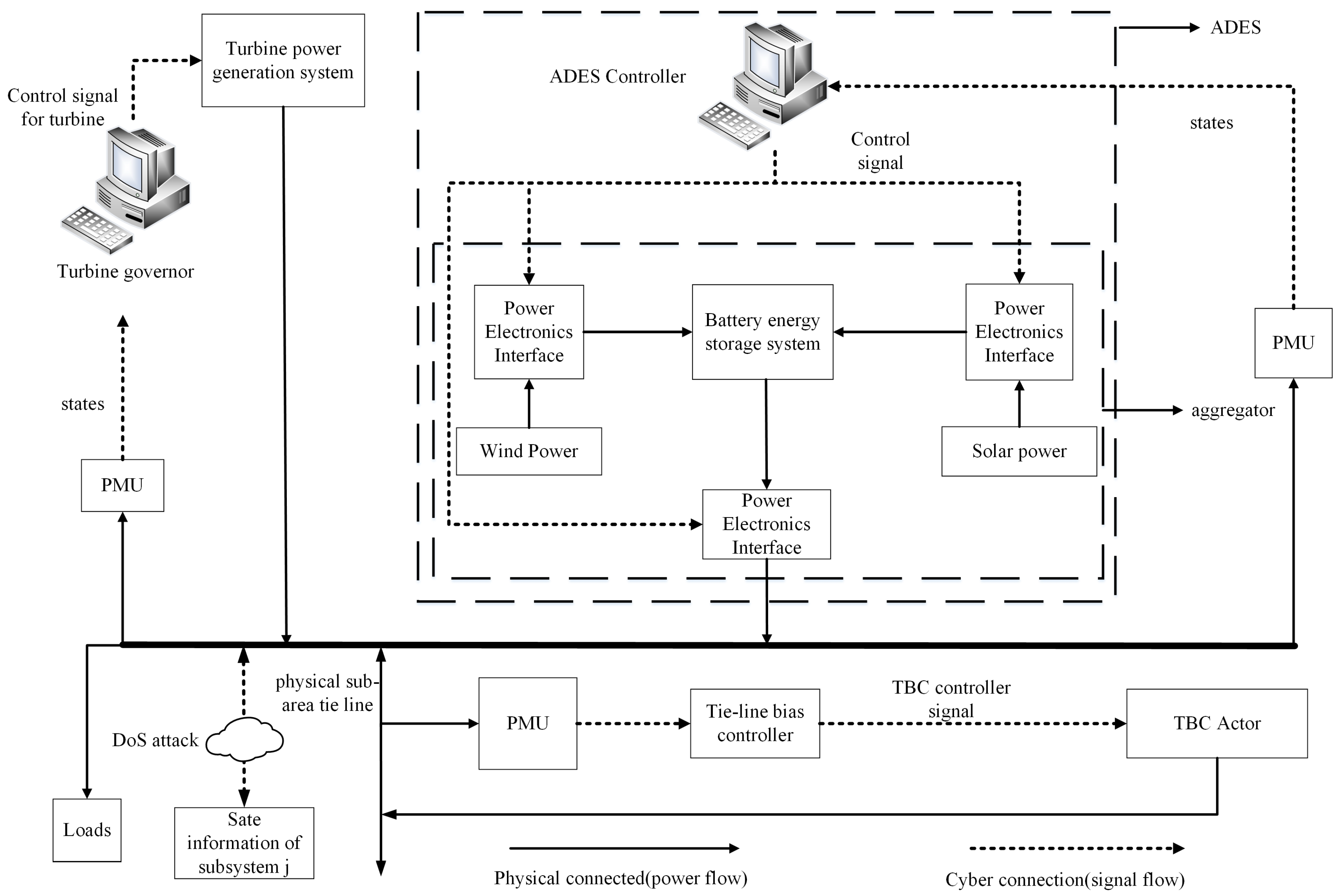
2. Load Frequency Control and DoS Attack Models Based on ADES

The development and popularization of distributed energy sources and power electronics techniques provide more flexible and efficient implementation methods for power grid frequency control [38]. The decentralized comprehensive energy utilization systems established in various regions compose an ADES system by integrating the power resources generated by different energy systems and transmitting them to large power grids [38].

As shown in Figure 1, if power grids are divided into multiple subsystems containing ADES, each subsystem transmits power and exchanges data information through power transmission lines and communication networks. Each subsystem includes phase measurement units (PMUs), ADES, ADES controllers, synchronous generators, turbine governors, tie-line controllers, power electronics interface, and the load. Renewable distributed energy sources, such as the electricity generated by wind and photovoltaics are smoothly output and connected to power grids through energy storage systems.

Due to disturbances, such as load changes, the power grid frequency fluctuates; therefore, the active power of synchronous generator sets is adjusted to control the power grid frequency based on the P-f droop control [44]. When the frequency deviation exceeds the set threshold range for the first time [45], ADES controllers are activated, and the battery energy storage system (BESS) is introduced to participate in the frequency adjustment process.

From now on, BESS continues to run. BESS has the ability of fast power response and four-quadrant operation, which can inject enough active power for the fast frequency adjustment of power grids under the disturbances of load changes. Renewable distributed energy sources have three main characteristics, randomness, intermittency, and volatility. If large-scale and high proportions of renewable distributed energy sources are connected to power grids, huge peaks and frequency regulation pressured occur, which weakens the system moment of inertia and brings new challenges to power grids, such as balance adjustment and safe and stable operations [46].

The proposed ADES-based strategy with BESS can realize the regional multi-energy aggregation mode in which the large-scale distributed energy resources are connected to power grids. There are two advantages to the ADES with BESS. First, the proposed strategy realizes the flexible control of large-scale distributed energy sources, and thus the scheduling of distributed energy sources can be processed as a whole.

Second, the proposed strategy is conducive to the rational and optimal allocation and utilization of energy resources [47]. This paper adopts controllable inverters as the interface and aggregation techniques, which have fast response speed, can effectively suppress frequency deviation in a short time and provide sufficient control capacity under aggregation and BESS to prevent the instability of power grids.

Each subsystem contains a local distributed ADES controller. When the subsystem ADES controller exerts a control function, the ADES controller first receives the PMU measurement data (the frequency and power deviation corresponding to the subsystem) from both local and other remote subsystems at each discrete sampling moment and then uses them to calculate the control output. The ADES controller also sends the corresponding control command signals to local distributed energy sources and adjusts the output power of each distributed energy system in real time to resist both frequency deviations and power grid oscillations.

DoS attacks occur in the information transmission process between subsystem i and subsystem j as shown in Figure 1. When DoS attacks occur, the information interaction between the two subsystems is cut off.

2.1. Load Frequency Control Model of Multi-Machine Power Grids

Suppose power grids are divided into sub-systems. In order to simplify both the system analysis and related applications, a linear dynamic model [48] is used to approximate the physical reference model of subsystems. The dynamic frequency control model of the subsystem $i (i=1,\dots ,N)$ can be expressed by the following discrete difference equations [49].

$$\begin{array}{c}\hfill {\mathit{x}}_i(k+1)={\mathbf{A}}_i{\mathit{x}}_i\left(k\right)+{\mathit{B}}_i{u}_i\left(k\right)+{\mathit{E}}_i{\varpi }_i\left(k\right)+\sum _{j\in \mathcal{N}\left(i\right)}{\mathbf{B}}_{ji}{\mathit{x}}_j\left(k\right)\end{array}$$

(1)

$$\begin{array}{cc}\hfill & {\mathit{B}}_i={\left(\begin{array}{cccccc}0& \Delta t/M_i& 0& 0& 0& 1-\Delta t/T_{Bi}\end{array}\right)}^{\mathrm{T}},{\mathit{E}}_i={\left(\begin{array}{cccccc}-\Delta t/M_i& 0& 0& 0& 0& 0\end{array}\right)}^{\mathrm{T}}\hfill \end{array}$$

(2)

$$\begin{array}{cc}\hfill & {\mathbf{B}}_{ji}=\left(\begin{array}{cccccc}0& 0& 0& 0& 0& 0\\ \frac{\Delta t{T}_{ij}}{M_i{\displaystyle \sum _{h\in D\left(i\right)}}{T}_{ih}}& 0& 0& 0& 0& 0\\ 0& 0& 0& 0& 0& 0\\ 0& 0& 0& 0& 0& 0\\ 0& 0& 0& 0& 0& 0\\ 0& 0& 0& 0& 0& 0\end{array}\right),{\mathit{x}}_i={\left(\Delta f_i\Delta P_{mi}\Delta P_{vi}\Delta P_{ji}\int AC{E}_i\Delta P_{Bi}\right)}^{\mathrm{T}}\hfill \end{array}$$

(3)

$$\begin{array}{cc}\hfill & {\mathbf{A}}_i=\left(\begin{array}{cccccc}0& 1-\Delta t{\sum }_{j\in D\left(i\right)}{T}_{ji}& 0& 0& 0& 0\\ 1+\frac{\Delta t}{M_i}& 1-\frac{D_i\Delta t}{M_i}& 1+\frac{\Delta t}{M_i}& 0& 0& 0\\ 0& 0& 1-\frac{\Delta t}{T_{di}}& \frac{\Delta t}{T_{di}}& 0& 0\\ 0& 1-\frac{\Delta t}{T_{gi}{R}_{gi}}& 0& 1-\frac{\Delta t}{T_{gi}}& 1-\frac{\Delta t{K}_i}{T_{gi}}& 0\\ 1& 1-\Delta t{b}_i& 0& 0& 0& 0\\ 0& 0& 0& 0& 0& 1-\frac{\Delta t}{T_{B_i}}\end{array}\right)\hfill \end{array}$$

(4)

where $i=1,\dots ,N$ is the subsystem number; $\mathcal{N}\left(i\right)$ is the collection of physically connected subsystems (power transmission line connection); $\Delta f_i$ is the frequency deviation of the subsystem i; $\Delta P_{mi}$ is the mechanical power deviation of the generator; $\Delta P_{vi}$ is the power deviation of the steam turbine; $\Delta P_{ji}$ is the power deviation of the tie line; $AC{E}_i$ is the area control error signal of system i; $AC{E}_i={\alpha }_i\Delta f_i+\Delta P_{ji}$, ${\mathbf{A}}_i$, ${\mathit{B}}_i$ are the state matrix of subsystem i and gain of the control input, respectively; k is the discrete sampling time; ${\mathbf{B}}_{ji}$ is the gain matrix of the state information of the subsystem j; ${\varpi }_i\left(k\right)$ is the load change disturbances of the subsystem i; ${\mathit{E}}_i$ is the disturbance gain; $T_{gi}$ is the inertia time constant of the turbine governor; $D_i$ is the damping coefficient; $T_{di}$ is the governor constant; $M_i$ is the constant of inertia; $R_{gi}$ is the inertia time coefficient of turbine adjustment; $T_{ji}$ is the synchronous inertia time constant between area connections; $b_i$ is the frequency deviation gain; $K_i$ is the deviation control gain of the tie line; and $\Delta t$ is the discrete sampling period.

Considering the BESS in the P-Q working mode, it assumes the dynamic model of the battery energy storage system as a first-order inertia link. $T_{Bi}$ in model (1) is the inertia time constant of the battery energy storage system. According to the P-Q droop control method, when the power grid load changes rapidly, active power needs to be injected to maintain the power balance of power grids.

The power injection of the BESS also changes all the time. Therefore, the active power deviation of the BESS also needs to be considered as the state information. $\Delta P_{Bi}$ is the active power deviation of the BESS. $u_i$ is the injected controllable active power provided by the BESS of the subsystem i as follows.

$$u_i\left(k\right)=\phi ({\mathit{x}}_i,{\mathit{x}}_{{\mathcal{N}}^{\prime }\left(i\right)})$$

(5)

where $\phi (.)$ is the control strategy, ${\mathit{x}}_i$, ${\mathit{x}}_{{\mathcal{N}}^{\prime }\left(i\right)}$ are the state information of the subsystem i and the remote network connection subsystem set ${\mathcal{N}}^{\prime }\left(i\right)$, respectively. The electric energy generated by both wind power and photovoltaic power is stored in the battery energy storage system through the power electronic interface, which is used to adjust the power balance of power grids.

However, due to the dynamic characteristics of the battery energy storage system, the output of the battery energy storage system is limited, and its response speed is also limited. In model (1), the active power deviation $P_{B_i}$ of the battery energy storage system must meet the following constraint.

$$\left|\Delta P_{B_i}\right|\le \Delta P_{B_i,lim}$$

(6)

where $\Delta P_{B_i,lim}$ is the maximum active power deviation to limit the injection.

2.2. Dynamic Model of Load Frequency Control Considering DoS Attacks

When power grids need ADES to provide frequency control service, hackers may launch DoS attacks against the communication network. DoS attacks take up a large amount of malicious communication network resources and block the transmission of remote state information between subsystems [50].

We assume that ${\delta }_{ji}\in \{0,1\}$ is the indicator variable of the state data packet loss caused by DoS attacks. At this time, the input of the ADES controller is $u_i\left(k\right)=\phi ({\mathit{x}}_i,{\delta }_{ji}{\mathit{x}}_{{\mathcal{N}}^{\prime }\left(i\right)})$. ${\delta }_{ji}$ at each sampling moment satisfies the Bernoulli probability distribution as follows.

$${\delta }_{ji}=\left\{\begin{array}{c}1,P\{{\delta }_{ji}=1\}=1-{\eta }_{ji}\hfill \\ 0,P\{{\delta }_{ji}=0\}={\eta }_{ji}\hfill \end{array}\right.$$

(7)

where the probability ${\eta }_{ji}$ of packet loss satisfies the following constraint.

$$\sum _{i=1}^N\sum _{j\in \mathcal{N}\left(i\right)\cap {\mathcal{N}}^{\prime }\left(i\right)}^{}{\eta }_{ji}\le \xi$$

(8)

The packet loss probability ${\eta }_{ji}$ is proportional to the intensity of DoS attacks [51]. $\xi$ as a fixed constant is the sum of packet loss probabilities between all communication connections.

Note. The above assumptions are reasonable. The communication network resources that attackers can use are limited. Communication network resources limit the attack intensity of DoS attacks. Therefore, the sum of the attack intensity of DoS attacks is considered to have a fixed upper bound, which means the sum of ${\eta }_{ji}$ is also considered to have a fixed upper bound.

They cause the ADES controller to lose some remote information ${\mathit{x}}_j\left(k\right)$ within a certain time period. The loss of remote information ${\mathit{x}}_j\left(k\right)$ may increase the control error, reduce the frequency error elimination speed, and even cause the frequency deviation of power grids to diverge, thereby, making the control strategy completely invalid.

Thus, in order to study the power grid frequency control strategy under DoS attacks, the following discrete dynamic model is established for multi-machine power grid frequency involving DoS attacks.

$$\begin{array}{c}\hfill {\mathit{x}}_i(k+1)={\mathbf{A}}_i{\mathit{x}}_i\left(k\right)+{\mathit{B}}_i{u}_i\left(k\right)+{\mathit{E}}_i{\varpi }_i\left(k\right)+\sum _{j\in \mathcal{N}\left(i\right)\cap {\mathcal{N}}^{\prime }\left(i\right)}{\delta }_{ji}{\mathbf{B}}_{ji}{\mathit{x}}_j\left(k\right)\end{array}$$

(9)

3. Optimized Load Frequency Control with Convex Neural Network-Based Reinforcement Learning

This paper proposes a power grid frequency control strategy of convex neural network-based reinforcement learning to solve the following three issues. (1) Communication networks of ADES controller among subareas suffer from DoS attacks. (2) Analytical modeling issues occur in the frequency control system design of large-scale and complex power grids. (3) The issues involve the fast optimization of a power grid frequency control strategy.

The actor–critic online reinforcement-learning structure is used to achieve both ADES-based power grid frequency control and disturbance suppression of DoS attacks. Convex neural networks are used to construct both actor and critic networks in the actor–critic structure algorithm. Convex neural networks can convert the nonlinear optimization problems in the critic networks into approximated convex relaxed optimization problems to avoid local optimization in the optimization process, and ensure that the actor networks can output suboptimal control output.

In addition, the convexity of the convex neural networks enables the training process of the actor networks to reach the convex point quickly as the gradient drops. In this case, the convergence speed of network weights is higher than that of general neural networks. The overall workflow of the power grid frequency control strategy of convex neural network-based reinforcement learning is shown in Figure 2.

In Figure 2, the frequency controller of each subsystem consists of both actor networks and evaluation networks. The critic networks are used to approximate the reinforced signal $Q_i\left(k\right)$, and the actor networks are used to approximate the optimal control strategy. The reinforced signal ${\widehat{Q}}_i\left(k\right)$ is used to optimize the actor networks, thereby, improving the control output $u_i\left(k\right)$.

Considering the impact of DoS attacks on communications, the proposed control strategy focuses on achieving the following two goals. (1) This control strategy can quickly dampen frequency fluctuations caused by sudden disturbances so that the power grid frequency deviation can be eliminated in a short time and so that the stability of power grids can be maintained. (2) This frequency control strategy can effectively resist the interference caused by DoS attacks.

Therefore, this paper adopts a load-frequency control strategy of convex neural network-based online reinforcement learning and uses BESS to eliminate the frequency deviation of power grids under DoS attacks. Additionally, online reinforcement learning can monitor the changes in the state of distributed power grid in real time, eliminate useless data blocked by DoS attacks, adjust the control output in real time, and provide the optimal control output for the state control of distributed energy grids, thereby, realizing real-time defense against DoS attacks.

The actor–critic structure is applied to the implementation of reinforcement learning. This paper introduces a convex neural network to approximate actor networks and critic networks. The introduction of convex neural network is shown below.

3.1. Convex Neural Network Structure Design

Finding the optimal control problem is converted to getting the control output or strategy that minimizes the long-term future cost $Q_i\left(k\right)$. However, the general direct search process for the long-term future cost $Q_i\left(k\right)$ is a non-convex problem. The existence of multiple local sub-optimal control strategies may not only lead to the inability to find the global optimal control strategy but also reduce the speed of optimization and convergence.

Therefore, this paper uses convex neural networks to build an approximated model of $Q_i\left(k\right)$. The optimization of reinforcement learning is carried out in the approximated model established by convex neural networks so that the optimization process of reinforcement learning is approximated as the convex optimization process.

In ordinary machine learning, convex generally means that the parameters are convex, and thus the weights are convex [40,52]. The convexity of convex neural networks means that the output is convex with respect to the input, while the network parameters are not fully convex. To make the output of convex neural networks be a convex function about the input, the convex neural networks need to meet the following constraints. (1) The weight matrix ${\mathbf{W}}_{1:N-1}^{\left(z\right)}$ of the middle layer of convex neural networks must be positive semi-definite. (2) All activation functions ${\varphi }_{m-1}(.)$ of convex neural networks are convex non-decreasing functions.

This paper defines a $Q_N$-layer neural network structure based on multiple inputs/outputs through recursive methods. The neural networks are called convex neural networks. The structure of the convex neural networks is shown in Figure 3. The convex neural networks consist of one input layer, N intermediate layers, and one output layer. The input layer is the state vector of each subsystem, which is denoted as ${\mathit{x}}_i^{\prime }={[{\mathit{x}}_1,{\mathit{x}}_2,\dots ,{\mathit{x}}_N]}^{\mathrm{T}}$.

Suppose the dimension of ${\mathit{x}}_i\left(k\right)$ is $l=6$. ${\widehat{\mathbf{W}}}_{m-1}^{\left(z\right)}\in {\mathbf{R}}^{Nl\times Nl}$ and ${\widehat{\mathbf{W}}}_{m-1}^{\left(y\right)}\in {\mathbf{R}}^{Nl\times Nl}$ are the weights of the middle layer, ${\mathbf{b}}_{m-1}\in {\mathbf{R}}^{Nl\times 1}$ is the bias of the middle layer, ${\widehat{h}}_m\in {\mathbf{R}}^{Nl\times 1}$ is the output vector of the m-th middle layer, $\widehat{o}$ is the output of the output layer, and ${\mathit{w}}_i\in {\mathbf{R}}^{1\times Nl}$ is the connection weight between the output layer and the last middle layer, $m=1,2\dots N$.

The output ${\mathit{h}}_m\in {\mathbf{R}}^{Nl\times 1}$ of the m-th middle layer can be expressed as follows.

$$\begin{array}{cc}\hfill & {\mathit{h}}_m={\varphi }_{m-1}({\mathbf{W}}_{m-1}^{\left(z\right)}{\mathit{h}}_{m-1}+{\mathbf{W}}_{m-1}^{\left(y\right)}{\mathit{x}}_i^{\prime }+{\mathit{b}}_{m-1})\hfill \\ \hfill & s.t.{\mathbf{W}}_{1:N-1}^{\left(z\right)}\ge \mathbf{0},{\mathbf{W}}_0^{\left(z\right)}\equiv \mathbf{0},{\mathit{h}}_{\mathbf{0}}\equiv \mathbf{0}\hfill \end{array}$$

(10)

where ${\varphi }_{m-1}(.)$ is the activation function $tanhx$ and ${\widehat{\mathbf{W}}}_{1:N-1}^{\left(z\right)}\ge 0$, ${\mathbf{W}}_0^{\left(z\right)}\equiv \mathbf{0}$ and ${\mathit{h}}_{\mathbf{0}}\equiv \mathbf{0}$ are the constraints. If and only if convex neural networks satisfy the above constraints, the output is the convex function of the input.

Suppose there is a set of weights ${\mathbf{W}}_i=\left\{{\mathbf{W}}_{0:N-1}^{\left(z\right)},{\mathbf{W}}_{0:N-1}^{\left(y\right)},{\mathit{w}}_i,{\mathit{b}}_{0:N-1}\right\}$. Then, the output layer of convex neural networks with respect to the output of middle layers can be expressed as follows.

$$\begin{array}{c}\hfill o={\mathit{w}}_i{\mathit{h}}_N=Con({\mathbf{W}}_i,{\mathit{x}}_i^{\prime })\end{array}$$

(11)

where $Con(.)$ represents the mapping function between input and output.

3.2. Critic Networks for Long Term Future Cost Approximation under DoS Attacks

Critic networks approximate the long-term future cost $Q_i\left(k\right)$ of the state trajectory under the current control strategy through the state information of power grids. The long-term future cost $Q_i\left(k\right)$ is the weighted sum of the instantaneous cost at each future moment. The instantaneous cost is a function of the current system state and control output.

This function not only considers the excessive frequency deviation but also measures the control cost. The long-term future cost output ${\widehat{Q}}_i\left(k\right)$ that evaluates the network approximation is the enhanced signal of reinforcement learning. Actor networks learn network parameters through the enhanced signal to reduce the control cost as much as possible and optimize the frequency control strategy by minimizing ${\widehat{Q}}_i$. The long-term future cost $Q_i\left(k\right)$ of the state trajectory can be defined as follows.

$$\begin{array}{cc}\hfill Q_i\left(k\right)& ={\alpha }^S{p}_i(k+1)+{\alpha }^{S-1}{p}_i(k+2)+\dots {\alpha }^{k+1}{p}_i\left(S\right)+\dots \hfill \end{array}$$

(12)

where $\alpha \in (0,1)$ is the decay rate, and $S\in Z+$ is a given positive integer for the long-term evaluation time window. $p_i\left(k\right)$ is the instantaneous cost function, and its value is related to the number of violations of the given frequency deviation threshold and the size of the optimal control output [38], which is defined as follows.

$$p_i\left(k\right)=\left\{\begin{array}{c}0,a_1∥{\mathit{x}}_i\left(k\right)∥+a_2∥u_i\left(k\right)∥\le c\hfill \\ 1,otherwise\hfill \end{array}\right.$$

(13)

where $∥•∥$ represents the 2-norm, $a_1$ and $a_2$ are the weights of the state and strategy utility functions, respectively, $a_1+a_2=1$, and c is the given cost threshold. When $p_i=0$, the power grids is in a good performance state at the k-th moment; when $p_i=1$, the power grids are in a bad performance state. Therefore, the control objective can be converted to the minimization of the long-term future cost $Q_i\left(k\right)$. Under the optimal state trajectory, an iterative formula for $Q_i$ [38] is shown as follows.

$$Q_i\left(k\right)=\alpha Q_i(k-1)-{\alpha }^{S+1}{p}_i\left(k\right)$$

(14)

In the control process, $Q_i\left(k\right)$ can be used as an enhanced signal to optimize the control output of the ADES controller of the i-th subsystem. However, $Q_i\left(k\right)$ cannot be directly analyzed and calculated without an analytical model. Therefore, this paper adopts approximation-learning based on convex neural networks. In order to improve the optimal search speed and efficiency of the learning algorithm, critic networks are constructed to approximate $Q_i\left(k\right)$. The critic networks can be expressed as follows.

$${\widehat{Q}}_i\left(k\right)=g_i({\mathit{x}}_i\left(k\right),u_i\left(k\right))$$

(15)

where ${\widehat{Q}}_i\left(k\right)$ is the approximate value of $Q_i\left(k\right)$ and $g_i(.)$ is the convex neural network function.

However, ${\mathit{x}}_i$ may be disturbed by DoS attacks, which may not be normal state information. In order to solve this problem, this paper adopts an approximate approach [53] to solve the impact of DoS attacks on the system state. The critic network will use the non-attacked state information at the previous moment to replace the attacked state information at the current moment.This approach can reasonably eliminate the impact of DoS attacks.

Suppose there is a set of weights ${\mathbf{W}}_{c,i}$, $g_i(.)$ that can be expressed as follows.

$$\begin{array}{c}\hfill g_i(.)=w_{c,i}{h}_{c,N}=Con\left({\mathbf{W}}_{c,i}{{\mathit{x}}^{\prime }}_i\right)\end{array}$$

(16)

where ${\mathbf{W}}_{c,i}=\left\{{\mathbf{W}}_{c,0:N-1}^{\left(z\right)},{\mathbf{W}}_{c,0:N-1}^{\left(y\right)},{\mathit{w}}_{c,i},{\mathit{b}}_{c,0:N-1}\right\}$.

The objective function of training $g_i$ can be constructed based on the TD-error of ${\widehat{Q}}_i\left(k\right)$ derived from Equation (15) under the optimal trajectory. The TD-error can be expressed as follows.

$$e_{c,i}\left(k\right)={\widehat{Q}}_i\left(k\right)-\alpha (\widehat{Q_i}(k-1)-{\alpha }^S{p}_i\left(k\right))$$

(17)

Therefore, according to the TD-error $e_{c,i}\left(k\right)$, the objective function used to evaluate network learning can be defined as follows.

$$E_{c,i}\left(k\right)=\frac{1}{2}{e_{c,i}}^{\mathrm{T}}\left(k\right)e_{c,i}\left(k\right)$$

(18)

3.3. Actor Networks for Control Strategy under DoS Attacks

Actor networks are used to calculate the control output $u_i\left(k\right)$ of the ADES controller. The input of the actor networks includes the state information of the local subsystem i and the remote network connection subsystem $j(j\in {\mathcal{N}}^{\prime }\left(i\right))$. This information is used for the learning of the actor networks and the calculation of the control output. The control output acts on the power electronics interface of power grids to eliminate sudden frequency fluctuations in power grids.

The evaluation signal output by the critic networks (also called the reinforced signal of reinforcement learning) can be used to select the optimal control output, but it may be difficult to stabilize the dynamic online learning process of power grids when the selection of the optimal control output only relies on the reinforced signal. Therefore, an expected control output is needed to measure the closeness between the output of the actor networks and the optimal control strategy of power grids.

According to the dynamic characteristics of power grids, the expected control output $u_{d,i}\left(k\right)$ is assumed to be used to improve the exponential stability and short-term performance of the system. The expected control output makes the power grids present certain stable dynamic characteristics and ensures that the state ${\mathit{x}}_i\left(k\right)$ of power grids approaches 0, and thus the dynamic characteristics of the power grids have the following form.

$${\mathit{x}}_i(k+1)={\mathbf{L}}_i{\mathit{x}}_i\left(k\right)+{\mathit{B}}_i\left[u_i\left(k\right)-u_{d,i}\left(k\right)\right]+{\mathbf{\chi }}_i$$

(19)

The expected control output $u_{d,i}\left(k\right)$ is the optimal controllable active power injected by the subsystem i. The frequency stability of the power grids is maintained through the balance of active power and reactive power. $u_{d,i}$ is expressed as follows.

$$\begin{array}{cc}\hfill u_{d,i}\left(k\right)& =-d_{f_i}\Delta f_i\left[1+M_i{\sum }_{j\in D_i}{T}_{ji}\right]-\left((M_i-D_i\Delta t)/\Delta t\right)\Delta P_{mi}\hfill \\ \hfill & -\left((M_i+\Delta t)/\Delta t\right)P_{vi}-{\sum }_{j\in \mathcal{N}\left(i\right)\cap {\mathcal{N}}^{\prime }\left(i\right)}\Delta P_{ji}\hfill \end{array}$$

(20)

where $d_{f_i}$ is a hypothetical positive real number. $u_{d,i}$ can satisfy the eigenvalue of ${\mathbf{L}}_i$ existing in the unit circle so that the state equation of the system is changed to Equation (1).

If the error between $u_i$ and $u_{d,i}$ is bounded, and the error ${\mathbf{\chi }}_i$ is bounded, the power grids are bounded and stable.

$${\mathbf{\chi }}_i={\sum }_{j\in \mathcal{N}\left(i\right)\backslash {\mathcal{N}}^{\prime }\left(i\right)}{\delta }_{ji}{\mathbf{B}}_{ji}{x}_j\left(k\right)+{\mathit{E}}_i{\varpi }_i\left(k\right)$$

(21)

According to the parameter $d_{f_i}$, the specific form of ${\mathbf{L}}_i$ can be expressed as Equation (22).

$${\mathbf{L}}_i=\left[\begin{array}{cccccc}0& 1-\Delta t{\sum }_{j\in D_i}{T}_{ji}& 0& 0& 0& 0\\ \begin{array}{c}1+\frac{\Delta t}{M_i}-\frac{d_{f_i}\Delta t}{M_i}\hfill \\ -d_{f_i}{\sum }_{j\in D_i}{T}_{ji}\Delta t\hfill \end{array}& 1& 0& 0& 0& 0\\ 0& 0& 1-\frac{\Delta t}{T_{di}}& \frac{\Delta t}{T_{di}}& 0& 0\\ 0& 1-\frac{\Delta t}{T_{gi}{R}_{gi}}& 0& 1-\frac{\Delta t}{T_{gi}}& 1-\frac{K_i\Delta t}{T_{gi}}& 0\\ 1& 1-b_i\Delta t& 0& 0& 0& 0\\ 0& 0& 0& 0& 0& 1-\frac{\Delta t}{T_{Bi}}\end{array}\right]$$

(22)

The control system focuses on reducing the frequency deviation $\Delta f_i$ to zero or constrains the change of $\Delta f_i$ to a fixed small interval as much as possible. However, due to the difficulty of analyzing and modeling a large system, such as power grids, traditional methods cannot directly calculate the expected control output $u_{d,i}\left(k\right)$. The approximation of the approximated $u_{d,i}\left(k\right)$ is denoted as $u_i\left(k\right)$.

In order to further optimize the long-term performance of the control strategy, this paper adds a reinforced signal ${\widehat{Q}}_{d,i}\left(k\right)$ as one of the evaluation signals to measure the control strategy. An additional evaluation error signal ${\widehat{Q}}_i\left(k\right)-{\widehat{Q}}_{d,i}\left(k\right)$ of the strategy utility function can be regarded as the reinforced signal of the critic networks to the actor networks.

When the approximated control output approximates the expected control output, the reinforced signal gradually approaches zero, and thus ${\widehat{Q}}_{d,i}$ is set to 0. Therefore, the objective function of training $\phi (.)$ can be represented by the error composed of the control error $\Delta u_i\left(k\right)$ and the reinforced signal $Q_i\left(k\right)$. Suppose there is a set of weights ${\mathbf{W}}_{a,i}$, ${\phi }_i(.)$ that can be expressed as follows.

$$\begin{array}{c}\hfill {\phi }_i(.)=u_{lim}tanh\left(w_{a,i}{h}_{a,N}\right)=u_{lim}tanh\left(Con({\mathbf{W}}_{a,i},{x^{\prime }}_i)\right)\end{array}$$

(23)

where ${\mathbf{W}}_{a,i}=\left\{{\mathbf{W}}_{a,0:N-1}^{\left(z\right)},{\mathbf{W}}_{a,0:N-1}^{\left(y\right)},{\mathit{w}}_{a,i},{\mathit{b}}_{a,0:N-1}\right\}$, and $u_{lim}$ is the maximum output constraint of $u_i$.

According to Equation (23), ${\phi }_i(.)$ is calculated by $u_{lim}tanh(.)$, and thus $u_i$ is constrained to $[-u_{lim},u_{lim}]$. Therefore, after passing through the inertia link of the battery energy storage system, $\Delta P_{B_i,lim}$ can also satisfy the Equation (6). The following two subsections introduce the basic structure and implementation of both critic networks and actor networks.

The error composed of the control error $\Delta u_i\left(k\right)$ and the reinforced signal ${\widehat{Q}}_i(k-1)$ output by the critic networks is expressed as follows.

$${\mathit{e}}_{a,i}\left(k\right)={\left[\sqrt{{\mathit{B}}_i}\Delta u_i\left(k\right),{\widehat{Q}}_i(k-1)\right]}^{\mathrm{T}}$$

(24)

where $\Delta u_i\left(k\right)=u_i\left(k\right)-u_{d,i}\left(k\right)$ is the error value between the approximated control output and the expected control output. Therefore, according to the error ${\mathit{e}}_{a,i}\left(k\right)$, the objective function for policy network learning can be defined as follows.

$$E_{a,i}\left(k\right)=\frac{1}{2}{{\mathit{e}}_{a,i}}^{\mathrm{T}}\left(k\right){\mathit{e}}_{a,i}\left(k\right)$$

(25)

The constant convexity of convex neural networks can ensure the existence of the global optimal solution in the reinforcement-learning optimization process [40], and prevent the optimization process from falling into the local optimum. Additionally, the robustness of convex neural networks is good when they are applied to solve optimization problems [41].

When power grids suffers from DoS attacks, the transmission of the state information ${\mathit{x}}_j$ of some remotely connected subsystems may be blocked. In the control process, both actor networks and critic networks deal with the blocked state information. The blocked state information is replaced by the state information of the previous moment rather than 0. Therefore, the estimation of the state information ${\mathit{x}}_j$ can be expressed as follows.

$${\widehat{\mathit{x}}}_j\left(k\right)=\left\{\begin{array}{c}{\mathit{x}}_j(k-1),{\delta }_{ji}=0,k>1\hfill \\ {\mathit{x}}_j\left(k\right),{\delta }_{ji}=1\hfill \end{array}\right.$$

(26)

As a main reason, the state information of each subsystem cannot quickly become 0 during normal operations. When the state information of a subsystem changes too much which induced noneligible estimation errors, the actor–critic networks can predict the reinforced signal and control output with the estimation errors since the robustness of the neural networks [53].

The optimization of state information is completely completed by the actor–critic networks. The impact of DoS attacks on state information is eliminated by the actor–critic networks. The actor network predicts the current state quantity based on the past state value. The predicted value is corrected by actor network parameters and system measurement values. Therefore, the issues of DoS attacks can be solved by reinforcement learning.

3.4. Critic-Actor Network Weight Learning

In order to make convex neural networks be able to approximate $u_{d,i}\left(k\right)$ and $Q_i\left(k\right)$ to the greatest extent (minimize the objective functions $E_{a,i}$ and $E_{c,i}$), the weight sets of both actor networks and critic networks need to be trained. ${\mathbf{W}}_{c,i}$ and ${\mathbf{W}}_{a,i}$ need to be updated to the optimal weight sets ${\mathbf{W}}_{c,i}^{*}$ and ${\mathbf{W}}_{a,i}^{*}$. According to $u_i\left(k\right)$, ${\widehat{Q}}_i\left(k\right)$ and the objective functions (18) and (25), the online learning algorithm of the weight set of convex neural networks can be obtained.

$\sqrt{{{\mathit{B}}_i}^{\mathrm{T}}}\sqrt{{\mathit{B}}_i}={\mathbf{1}}^{\mathrm{T}}{\mathit{B}}_i$ is defined, where $\mathbf{1}={[1,1,1,1,1,1]}^{\mathrm{T}}$. Thus, Equation (25) can be expanded as follows.

$$\begin{array}{cc}\hfill & E_{a,i}\left(k\right)=\frac{1}{2}{\mathit{e}}_{a,i}{\left(k\right)}^{\mathrm{T}}{\mathit{e}}_{a,i}\left(k\right)=\frac{1}{2}{\mathbf{1}}^{\mathrm{T}}{\mathit{B}}_i\Delta u_i^2\left(k\right)+\frac{1}{2}{\widehat{Q}}^2(k-1)\hfill \end{array}$$

(27)

where $\Delta u_i\left(k\right)=u_i\left(k\right)-u_{d,i}\left(k\right)$. However, some parameters in the expected control output $u_{d,i}\left(k\right)$ are unknown; therefore, $\Delta u_i\left(k\right)$ cannot be directly expressed by this formula. Thus, ${\mathit{B}}_i\Delta u_i\left(k\right)$ is indirectly expressed by Equation (1). ${\mathit{B}}_i\Delta u_i\left(k\right)={\mathit{x}}_i(k+1)-{\mathbf{L}}_i{\mathit{x}}_i\left(k\right)-{\mathbf{\chi }}_i$.

For the objective function of critic network (18), it is expanded as follows.

$$\begin{array}{cc}\hfill E_{c,i}\left(k\right)=& \frac{1}{2}{e}_{c,i}{\left(k\right)}^{\mathrm{T}}{e}_{c,i}\left(k\right)=\frac{1}{2}{\left[{\widehat{Q}}_i\left(k\right)-\alpha ({\widehat{Q}}_i(k-1)-{\alpha }^S{p}_i\left(k\right))\right]}^2=\frac{1}{2}{\widehat{Q}}_i^2\left(k\right)+\frac{1}{2}{\alpha }^2{\widehat{Q}}_i^2(k-1)\hfill \\ \hfill & +\frac{1}{2}{\alpha }^{2(S+1)}{p}_i^2\left(k\right)-\alpha {\widehat{Q}}_i\left(k\right){\widehat{Q}}_i(k-1)-{\alpha }^S{p}_i\left(k\right){\widehat{Q}}_i\left(k\right)+{\alpha }^{S+1}{p}_i\left(k\right){\widehat{Q}}_i(k-1)\hfill \end{array}$$

(28)

The update process of the weight sets ${\mathbf{W}}_{a,i}\left(k\right)$ and ${\mathbf{W}}_{c,i}\left(k\right)$ depends on the gradient descent algorithm. However, only using the gradient descent method to update the weights of actor–critic networks cause some problems. Since ${\mathbf{W}}_i\left(k\right)$ needs to meet certain constraints, if only the gradient descent method is used in the learning process to update the weights of actor–critic networks, the updated network weights may not be able to maintain within the constraint set.

Therefore, it is necessary to ensure that the weight set after the gradient descent update always falls in the feasible region (non-negative weight). The projected gradient algorithm is used to ensure that the weight constraints are maintained. The projection of matrix ${\mathbf{W}}^{\prime }$ on the constraint set $\mathsf{\Omega }$ is defined as follows.

$${\Pi }_{\mathsf{\Omega }}\left({\mathbf{W}}^{\prime }\right)=\underset{\mathbf{W}\in \mathsf{\Omega }}{argmin}\frac{1}{2}{∥\mathbf{W}-{\mathbf{W}}^{\prime }∥}_F^2$$

(29)

where $\mathsf{\Omega }$ is the constraint set of the weights of convex neural networks, $\mathsf{\Omega }=\left\{{\mathbf{W}}_i|{\mathbf{W}}_{1:N-1}^{\left(z\right)}\ge \mathbf{0}\right\}$.

Given the initial weight state ${\mathbf{W}}_{1:N-1}^{\left(z\right)}\left(0\right)\in \mathsf{\Omega }$, the learning rates $0<\beta <1$ and $0<\gamma <1$ of actor–critic network weights, the projected gradient descent method extends the standard gradient descent to a feasible set $\mathsf{\Omega }$. Therefore, based on the projected gradient descent method, the update rules of ${\mathbf{W}}_{a,i}\left(k\right)$ and ${\mathbf{W}}_{c,i}\left(k\right)$ at time k can be expressed as follows.

$$\begin{array}{cc}\hfill & {\mathbf{W}}_{a,i}(k+1)={\mathbf{W}}_{a,i}\left(k\right)-\beta {\Pi }_{\mathsf{\Omega }}\left(\frac{\partial E_{a,i}\left(k\right)}{\partial {\mathbf{W}}_{a,i}\left(k\right)}\right),{\mathbf{W}}_{c,i}(k+1)={\mathbf{W}}_{c,i}\left(k\right)-\gamma {\Pi }_{\mathsf{\Omega }}\left(\frac{\partial E_{c,i}\left(k\right)}{\partial {\mathbf{W}}_{c,i}\left(k\right)}\right)\hfill \end{array}$$

(30)

According to Equations (27) and (28), $\partial E_{a,i}\left(k\right)/\partial {\mathbf{W}}_{a,i}\left(k\right)$ and $\partial E_{c,i}\left(k\right)/\partial {\mathbf{W}}_{c,i}\left(k\right)$ can be calculated. Therefore, the update rules of the actor–critic network weight set can be re-expressed as follows.

$$\begin{array}{cc}\hfill {\mathbf{W}}_{a,i}(k+1)& ={\mathbf{W}}_{a,i}\left(k\right)-\beta u_{lim}\times {\Pi }_{\mathsf{\Omega }}\left({\mathbf{1}}^{\mathrm{T}}\left[{\mathit{x}}_i(k+1)-{\mathbf{L}}_i{\mathit{x}}_i\left(k\right)\right]\right.\left.\left[1-{tanh}^2\left({\mathbf{W}}_{a,i}\left(k\right)\right)\right]{\mathit{w}}_{a,i}^{\mathrm{T}}\right)\hfill \\ \hfill {\mathbf{W}}_{c,i}(k+1)& ={\mathbf{W}}_{c,i}\left(k\right)-\gamma \times {\Pi }_{\mathsf{\Omega }}\left(\left[{\widehat{Q}}_i\left(k\right)-\alpha {\widehat{Q}}_i(k-1)-{\alpha }^S{p}_i\left(k\right)\right]\right.\left.\left[1-{tanh}^2\left({\mathbf{W}}_{c,i}\left(k\right)\right)\right]{\mathit{w}}_{c,i}^{\mathrm{T}}\right)\hfill \end{array}$$

(31)

This projected gradient descent method can make the convex neural network weights always meet the constraint conditions and avoid the divergence of the actor–critic networks caused by the weights crossing the feasible set $\mathsf{\Omega }$.

3.5. Analysis of Power Grid Stability and Convergence of Convex Neural Network Weights

Equation (31) is used to learn the parameters of both actor networks and critic networks. Equation (22) satisfies the stability requirements of the aggregated distributed energy grids. When the parameters $\beta$ and $\gamma$ and the maximum absolute value of the eigenvalue ${\lambda }_{max}\left({\mathbf{L}}_i\right)|$ of the matrix ${\mathbf{L}}_i$ are selected appropriately, the proposed control strategy can achieve good control performance.

In the following stability analysis, the overall system stability is indirectly proved by analyzing the subsystem stability. In the analysis of subsystem stability, the interconnection influence between subsystems is considered. If all the subsystems are stable, the overall system is stable. Thus, the stability of the subsystems is consistent with the stability of the overall system. The consideration of interconnection influence in the discussion of subsystem stability is reflected in the following four aspects.

• The expected control output $u_{d,i}$ designed in this paper and the gain term $M_i{\sum }_{j\in D_i}{T}_{ji}$ of the physical interconnection disturbances included in the subsystem model (1) are involved.
• The expected output of subsystem control $u_{d,i}$ and the calculation of actual control output including the variable set ${\mathit{x}}_{{\mathcal{N}}^{\prime }\left(i\right)}$ of information adjacent subsystems are involved.
• The modeling and estimation error term ${\chi }_i$ in model (9) include the estimation error relationships of physical and information interconnection disturbances between subsystems.
• When convex neural networks are used to approximate the critic networks and actor networks of reinforcement learning, the approximation errors ${\epsilon }_{a,i}$ and ${\epsilon }_{c,i}$ of convex neural networks are also considered. These two errors also include the estimation error relationships of physical and information interconnection disturbances between subsystems.

In order to theoretically analyze the stability of the aggregated distributed energy grids and the convergence of the actor–critic network weights, the following assumptions are made.

Assumption 1.

The activation function ${\varphi }_i(.)$ is a non-decreasing and non-constant function that satisfies the global Lipschitz condition, and there is a positive number that satisfies the following inequality.

$$\begin{array}{c}\hfill 0\le ∥{\varphi }_i({\mathbf{W}}_i,{\mathit{x}}_i)-{\varphi }_i({\mathbf{W}}_i^{*},{\mathit{x}}_i)∥\le L{}_i^{\prime }∥{\mathbf{W}}_i-{\mathbf{W}}_i^{*}∥\end{array}$$

where ${\mathbf{W}}_i={\mathbf{W}}_{a,i}$, ${\mathbf{W}}_i^{*}={\mathbf{W}}_{a,i}^{*}$, or ${\mathbf{W}}_i={\mathbf{W}}_{c,i}$, ${\mathbf{W}}_i^{*}={\mathbf{W}}_{c,i}^{*}$. The smallest possible $L{}_i^{\prime }$ that satisfies the above inequality is called the Lipschitz constant of the function ${\varphi }_i(.)$.

Note. For a non-decreasing and non-constant function, if there is a continuous derivative at any point in a fixed domain, the function must satisfy the Lipschitz condition in the domain. The activation function ${\varphi }_i(.)=tanhx$ is a monotonically increasing function in a fixed continuous domain, and there is a continuous derivative at any point in the domain. Therefore, the activation function ${\varphi }_i(.)$ satisfies the Lipschitz condition.

Assumption 2.

Assume that the vectors ${\mathit{w}}_{a,i}$ and ${\mathit{w}}_{c,i}$ in the weight sets ${\mathbf{W}}_{a,i}$ and ${\mathbf{W}}_{c,i}$, and the control gain ${\mathit{B}}_i$ in the system model of aggregated distributed energy grids satisfy the following equation and inequality.

$$\begin{array}{c}\hfill ∥{{\mathit{w}}_{a,i}}^{\mathrm{T}}{\mathit{w}}_{a,i}∥=∥{{\mathit{w}}_{c,i}}^{\mathrm{T}}{\mathit{w}}_{c,i}∥=1,0\le ∥{\mathit{B}}_{i,min}∥\le ∥{\mathit{B}}_i∥\le ∥{\mathit{B}}_{i,max}∥\end{array}$$

Note. This assumption is reasonable. On the one hand, the vectors ${\mathit{w}}_{a,i}$ and ${\mathit{w}}_{c,i}$ are given constant vectors, and they are set as the vectors that satisfy Assumption 2 during the parameter initialization. On the other hand, ${\mathit{B}}_i$ is the power input gain of distributed energy sources that affects future frequency deviation changes, and the gain is limited.

Assumption 3.

There is a matrix ${\mathbf{P}}_i$ that makes the projection of matrix ${\mathbf{W}}^{\prime }$ on the constraint set Ω be expressed as ${\Pi }_{\mathsf{\Omega }}\left({\mathbf{W}}^{\prime }\right)={\mathbf{P}}_i{\mathbf{W}}^{\prime }=\mathbf{W}$, and ${\mathbf{P}}_i$ satisfies $∥{\mathbf{P}}_{i,\min }∥\le ∥{\mathbf{P}}_i∥\le ∥{\mathbf{P}}_{i,\max }∥$.

Note. The above assumption is feasible. Matrix projection can be expressed as projecting the matrix column space composed of matrix column vectors into another matrix column space. Projection from a certain matrix column space to another matrix column space can be completed by linear transformation. Thus, there is a certain matrix that makes the matrix column space project to another matrix column space after linear transformation. Moreover, the dimension of the projection matrix is related to the size of the matrix column space. When the dimension of the projection matrix is limited, the norm of the projection matrix must have an upper bound and a lower bound [54].

Based on the above assumptions, this section presents the sufficient conditions for the stability of the aggregated distributed energy grids and the actor–critic network weight convergence to meet the ultimate uniformly bounded (UUB) stability. This sufficient condition strictly gives the controller parameters and adaptive gain range. Within this range, power grids belong to UUB under the disturbances of DoS attacks and load changes, and the weights of convex neural networks can also converge as shown in Theorem 1.

Theorem 1.

If the parameters of aggregated distributed energy grids, actor networks and critic networks satisfy the inequality group (32), then the set of weights ${\tilde{\mathbf{W}}}_{a,i}$, ${\tilde{\mathbf{W}}}_{c,i}$ and the system state ${\mathit{x}}_i\left(k\right)$ are UUB and stable.

$$\left\{\begin{array}{c}2\left[{∥{\mathbf{P}}_{a,i,max}∥}_F^2\left({\beta }^2-\beta \right)u_{lim}^2+2\right]\times L{{}_i^{\prime }}^2{∥{\mathit{B}}_{i,\mathit{max}}∥}^2{u}_{lim}^2<\beta ,\hfill \\ 4{∥{\mathbf{P}}_{c,i,max}∥}_F^{2}L{{}_i^{\prime }}^2\left({\gamma }^2-\gamma \right)-\gamma <0,\hfill \\ 2{∥{\mathbf{L}}_i∥}^2-1<0,0\le \left|{\lambda }_i\left({\mathbf{L}}_i\right)\right|\le 1,\hfill \\ \beta >0,\gamma >0\hfill \end{array}\right.$$

(32)

where ${∥{\mathbf{P}}_{c,i,max}∥}_F^2$ and ${∥{\mathbf{P}}_{c,i,max}∥}_F^2$ are the squares of the maximum F norm of matrix ${\mathbf{P}}_{a,i}$ and matrix ${\mathbf{P}}_{c,i}$, respectively, and $\left|{\lambda }_i\left({\mathbf{L}}_i\right)\right|$ is the absolute value of the eigenvalue of matrix.

The proof of Theorem 1 is given in the Appendix A.

There is still a certain error in using convex neural networks to approximate actor–critic networks. The reason is that a certain error range exists in the training process of convex neural network weights. When the target learning functions $E_{a,i}\left(k\right)$ and $E_{c,i}\left(k\right)$ are within the error range, the network weights are no longer updated. This error does not affect the global stability of aggregated distributed energy grids and the convergence of the weights of actor–critic networks.

4. Experiment Environment

This paper uses IEEE14, IEEE57 and IEEE118 bus testing systems [54] to verify the effectiveness of the proposed control strategy. The adaptability of the proposed frequency control strategy is explored under different DoS attack intensities. The convergence of the proposed strategy is compared with the convergence of other actor–critic networks. The effectiveness and superiority of the proposed frequency control strategy is discussed. The IEEE118 bus testing system is used to analyze the generalization ability of the proposed frequency control strategy.

All experiments were simulated using Matlab2016A on a desktop with Intel i7-6700k [email protected] GHz and 48 GB memory.

4.1. Configuration of System Model and Learning Parameters

According to the power grid toolbox MATPOWER [54] installed on MATLAB, the relevant data about the IEEE14, IEEE57, and IEEE118 bus testing systems were obtained. The related data include the physical topology of node networks, admittance and power information. The IEEE14 bus testing system consists of five generator buses and nine load buses, in which bus 1 is a balanced bus. IEEE57 bus testing system consists of seven generator buses and 50 load buses, in which bus 1 is a balanced bus.

IEEE118 bus testing system consists of 54 generator buses and 64 load buses, in which bus 69 is a balanced bus. The IEEE14, IEEE57, and IEEE118 bus test systems are divided into two, three, and five areas, respectively. Each area is equipped with an independent controller. The controller of each area controls the buses of this area, respectively. As shown in

Table 1. Bus parameters.

Parameter Name	Description	Value
$M_i$	inertia constant	0.05
$D_i$	damping constant	0.002
$T_{gi}$	gas turbine constant	0.2
$T_{di}$	governor constant	5
$R_{gi}$	regulation constant	0.5
$T_{ji}$	synchronizing constant	0.5
$T_{Bi}$	Inertial time constant of BESS	0.5
$b_i$	frequency bias gain	1
$K_i$	tie-line bias control gain	0.1

, the relevant parameter values of the kinetic model (1) of each bus are initialized. The sampling time $\Delta t$ is set to 10 ms.

The vector $v_{ji}\in {\mathbf{R}}^{N\times 1}$ is used to approximate the indicator variable ${\delta }_{ji}$ of DoS attacks, and its value is 0 or 1. In this vector, the number of 0 and 1 is related to the probability of data packet loss ${\eta }_{ji}$. DoS attacks satisfy Equation (8).

For the three bus testing systems, their performance is evaluated under load change disturbances. Assuming that the load change disturbances ${\varpi }_i\left(k\right)$ of each bus satisfies $∥{\varpi }_i\left(k\right)∥\le 0.2$ pu [55], it changes once every 0.5 s. Figure 4 shows the multi-step load change disturbances curves on buses 1, 5, 9, and 14.

In the following experiments, the starting time of the ADES controller is set as the time when the controller detects that the frequency deviation of power grids exceeds $\pm 0.2$ rad/s ($\pm 0.03$ Hz) for the first time [56]. After that, the ADES controller controls the frequency control process of BESS acting on power grids.

4.2. Validation of the Strategy

In order to verify the effectiveness of the proposed frequency control algorithm under load change disturbances and DoS attacks, this subsection discusses the frequency deviation changes of power grids without the designed ADES controller. IEEE14 bus testing system is used for simulation. Assuming that the probability of data packet loss caused by DoS attacks is ${\eta }_{ji}=0.05$, the attack period is 1–1.3 s, and the duration is 300 ms.

If there is no ADES controller for auxiliary frequency control (the ADES controller is set not to participate in the frequency modulation process of power grids), the active power injected by BESS into power grids is $\Delta P_{B_i}=0$. As shown in Figure 5 and Figure 6, the frequency deviation change curve of the testing system and the current generator output curve can be obtained only by the active output adjustment of the generator participating in the frequency modulation process of power grids.

As shown in Figure 5, the frequency of each bus presents an oscillating state under the influence of load change disturbances. In the control process, the power generation end participates in the frequency adjustment process by controlling the power output of the generator to weaken the influence of the load change on frequency deviation. However, the frequency deviation still exceeds its threshold 0.03 Hz at the end of the control process. Thus, ADES needs to be introduced to control the frequency deviation of power grids.

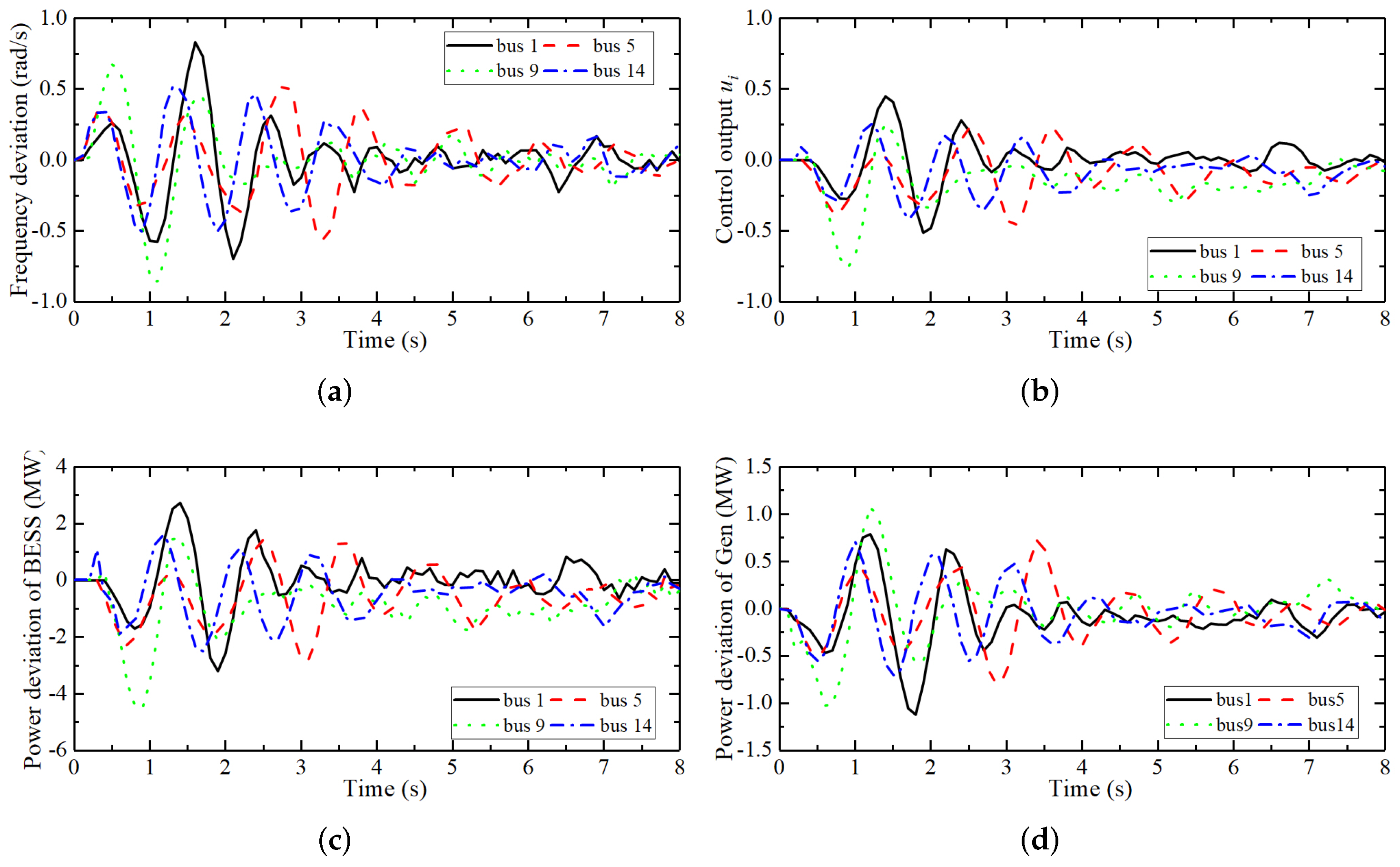
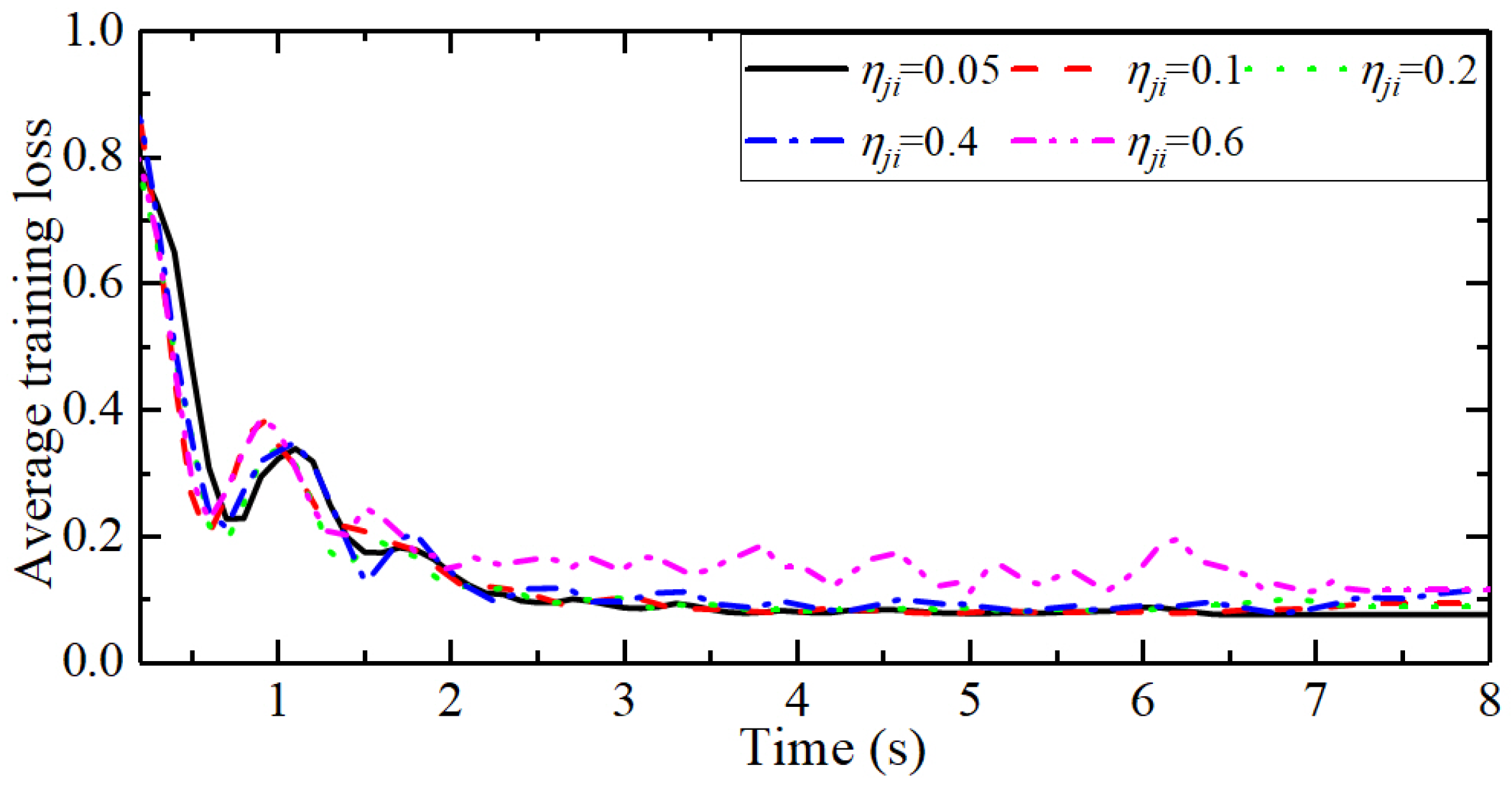
4.3. Case 1: Frequency Control of the IEEE 14-Bus Testing System under Different DoS Attack Intensities

IEEE14 bus testing system is used to verify the effectiveness of the proposed control strategy under load change disturbances and different data packet loss rates. ${\eta }_{ji}\in \left\{0.05,0.1,0.2,0.4,0.6\right\}$ is set. Both DoS attack period and total attack time under different ${\eta }_{ji}$ are shown in

Table 2. DoS attack period and total attack time under different data packet loss rates.

${\mathit{\eta }}_{\mathit{ji}}$	Attack Time	Total Attack Time
0.05	1–1.3 s.	0.3 s
0.1	1–1.3 s, 7.2 s–7.4 s.	0.5 s
0.2	1–1.3 s, 2 s–2.2 s,	1 s
	3 s–3.5 s.
0.4	1–1.3 s, 1.6 s–2 s,	1.1 s
	3 s–3.2 s, 7.2 s–7.4 s.
0.6	1.3 s–1.5 s, 2 s–2.5 s,	1.9 s
	3 s–4 s, 6.3 s–6.5 s,
	7.2 s–7.4 s.

.

As shown in

Table 3. Learning parameters of the IEEE14 bus testing system.

Parameter Name	Description	Value
$\beta$	learning rate of critic networks	0.001
$\gamma$	learning rate of actor networks	0.009
N	number of input neurons	14
$\xi$	sum of attack threshold	6
$Q_N$	number of network layers	16
$|{\lambda }_{max}\left({\mathbf{L}}_i\right)|$	the maximum absolute value of ${\mathbf{L}}_{\mathbf{i}}$	0.4
${∥{\mathit{B}}_{i,max}∥}^2$	the maximum value of ${∥{\mathit{B}}_i∥}^2$	0.015
$L_i^{\prime }$	Lipschitz constant	1
$a_1$	the weight of $x_i\left(k\right)$	0.7
$a_2$	the weight of $u_i\left(k\right)$	0.3
$\alpha$	damping factor	0.8
S	long-term evaluation time windows	10
$u_{lim}$	the maximum constraint of $u_i$	2.0
$\Delta P_{B_i,lim}$	the maximum constraint of $\Delta P_{B_i}$	25 MW

, the values of ADES controller parameters are initialized, including the learning rate of convex neural network weight update $\beta$ and $\gamma$, the number of subsystems N, the number of network layers of convex neural networks $Q_N$, the maximum absolute value $|{\lambda }_{max}\left({\mathbf{L}}_i\right)|$ of the eigenvalue of matrix ${\mathbf{L}}_i$, ${∥{\mathit{B}}_{i,max}∥}^2$, Lipschitz constant $L_i^{\prime }$, the weight $a_1$ of the state ${\mathit{x}}_i\left(k\right)$, the weight $a_2$ of the strategy $u_i\left(k\right)$, the attenuation factor $\alpha$, the number of long-term evaluation time windows S, the Lipschitz constant of the function $tanhx$, the maximum constraint of the control output $u_{lim}$ and the maximum constraint of $\Delta P_{B_i}$.

These initialization parameters all satisfy the power grid stability and the sufficient conditions for the convergence of the actor–critic network weights Equation (32). ${\mathit{w}}_{a,i}$ and ${\mathit{w}}_{c,i}$ are initialized as vectors that satisfy the Assumption 2, and the simulation time is 8 s. The experimental results are shown in Figure 7, Figure 8, Figure 9, Figure 10, Figure 11 and Figure 12. As shown in Figure 7, Figure 8, Figure 9, Figure 10 and Figure 11, subfigure (a) shows the frequency deviation curve, subfigure (b) shows the change curve of the control output $u_i$, subfigure (c) shows the deviation curve of the BESS power output.

The power output of BESS is determined by the control output $u_i$. There is a first-order inertia relationship between BESS and $u_i$. Therefore, the output of Bess can be expressed through the first-order inertia link. Subfigure (d) shows the generator power output curve. Figure 12 shows the average loss curve of the weight training of convex neural networks under different data packet loss rates.

The stabilization time is defined as the time required for the frequency deviation to remain within a fixed interval after being adjusted by the ADES controller. Assuming that the stable interval is $\pm 0.1$ rad/s ($\pm 0.1$ Hz), when the frequency deviation of all buses is maintained between $\pm 0.01$ Hz, the system has been recovered to its nominal operating state [56].

As shown in Figure 7a,b, the frequency deviations of buses 1, 5, 9, and 14 exceed the frequency deviation threshold Hz at 0.4, 0.3, 0.7, and 0.5 s, respectively. At this time, the ADES controller starts and generates $u_i$ (shown in Figure 7b) to control the active power output of BESS. The power changes of BESS are shown in Figure 7c. At the same time, the generator end also participates in frequency control, and the power change curve of the generator is shown in Figure 7d. In the simulation process, the maximum frequency deviation is 0.1 Hz, and each bus enters a stable state after about 4.3 s and finally shows small fluctuations in the stable interval.

As shown in Figure 8a,b, the frequency deviations of buses 1, 5, 9, and 14 exceed the frequency deviation threshold Hz at 0.3, 0.3, 0.4, and 0.3 s, respectively. At this time, the ADES controller starts and generates $u_i$ (as shown in Figure 8b). BESS is introduced to participate in the power grid frequency control process. The power deviation curve of BESS is shown in Figure 8c, and the power change curve of the generator is shown in Figure 8d. In the simulation process, the maximum frequency deviation is 0.12 Hz, buses 1, 5, 9, and 14 become stable at 3.4, 3.8, 3.4, and 4.5 s, respectively. Under the influence of load disturbances, the frequency deviation eventually fluctuates in the stable interval.

As shown in Figure 9a,b, the frequency deviations of buses 1, 5, 9, and 14 exceed the frequency deviation threshold Hz at 0.4 s, 0.7 s, 0.3 s, and 0.4 s, respectively. At this time, the ADES controller starts and generates $u_i$ (shown in Figure 9b) to adjust the active power output of BESS. The power deviation curves of BESS are shown in Figure 9c, and the power change curves of the generator are shown in Figure 9d. During the simulation process, the maximum frequency deviation is 0.11 Hz, bus 1 tends to be stable at 3.7 s, and buses 5, 9, 14 tend to be stable at 4 s. Due to the load disturbances, the frequency deviation eventually fluctuates in the stable interval.

As shown in Figure 10a,b, the frequency deviations of buses 1, 5, 9, and 14 exceed the frequency deviation threshold Hz at 0.3, 0.3, 0.3, and 0.4 s, respectively. At this time, the ADES controller starts, and the output $u_i$ (shown in Figure 10b) is used to adjust the active power output of BESS. The power change curves of BESS are shown in Figure 10c, and the power change curves of the generator are shown in Figure 10d.

The increase in the intensity of DoS attacks results in the adaptive increase or decrease of the change range of $u_i$, thereby suppressing the interference caused by DoS attacks to the frequency control process of power grids. During the simulation process, the maximum frequency deviation is 0.09 Hz, the stabilization time of buses 1, 5, 9, and 14 is 3.4, 3.5, 3.2, and 4 s, respectively. The frequency deviation of each bus eventually fluctuates in the stable interval.

The maximum frequency deviation in Figure 11a is 0.13 Hz. During the simulation process, each bus has an oscillating trend inside and outside the stable interval and cannot converge to the stable interval. At this time, the control output (shown in Figure 11b), the power output deviation of BESS (shown in Figure 11c), and the power output deviation of the generator (shown in Figure 11d) also present an oscillating state with a large change range, respectively. Since the intensity of DoS attacks is too strong, each bus cannot obtain the state information from the adjacent buses. The ADES controller cannot accurately calculate the control output.

As shown in Figure 12, the average training loss decreases gradually, as the data packet loss rate ${\eta }_{ji}$ continues to increase. Compared with other values of ${\eta }_{ji}$, the oscillation amplitude of the average training loss of convex neural network weights is larger when ${\eta }_{ji}=0.6$. When the intensity of DoS attacks increases, the convergence speed of convex neural network weights decreases. After experimental calculations, each weight update time is about 6 ms (less than the sampling time 10 ms), and thus the control strategy update can be completed within one sampling time.

According to the above experimental results, the proposed frequency control strategy can complete power grid frequency adjustment under a variety of DoS network attack intensity and load disturbances, and restrain the impact of load change disturbances on power grid frequency.

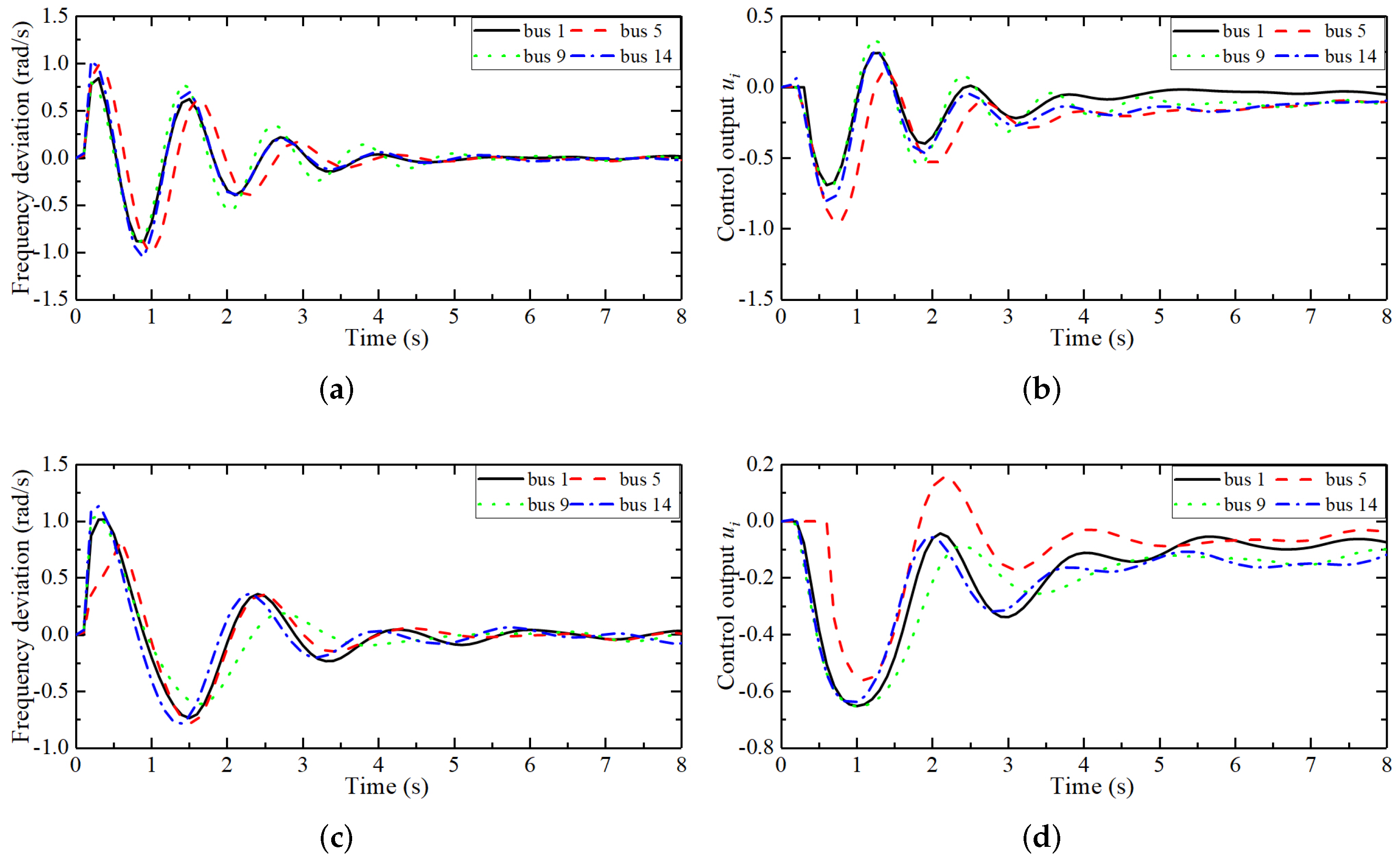
4.4. Case 2: Comparative Analysis of Frequency Control Effects of Different Methods under DoS Attacks

In the process of reinforcement learning, this paper uses convex neural networks to establish an approximate model of critic networks, and fast optimization of reinforcement learning is carried out in the approximate model established by convex neural networks. Thus, the optimization process of reinforcement learning is approximated as the convex optimization process.

In order to verify that the frequency control strategy based on convex neural networks is better than the frequency control strategy based on general neural networks, this section first uses two types of traditional neural networks (radial basis function neural networks (RBF) [38] and recurrent neural networks (RNN) [26]) to approximate critic networks in reinforcement learning. Then, the proposed frequency control strategy is compared with them to analyze the control performance of the frequency control strategies constructed by different neural networks under load change disturbances and DoS attacks.

Under three different DoS attack intensities, the IEEE57 bus testing system is used to verify the control performance of three methods on power grid frequency and the adaptability to different DoS network attack intensities.

The model parameters of the IEEE57 bus testing system are shown in Table 1, and the initialized parameters of the corresponding ADES controller are shown in

Table 4. Learning parameters of the IEEE 57 bus testing system.

Parameter Name	Description	Value
$\beta$	learning rate of critic networks	0.0025
$\gamma$	learning rate of actor networks	0.0011
N	number of input neurons	57
$\xi$	sum of attack threshold	22
$Q_N$	number of network layers	59
$|{\lambda }_{max}\left({\mathbf{L}}_i\right)|$	the maximum absolute value of ${\mathbf{L}}_{\mathbf{i}}$	0.4
${∥{\mathit{B}}_{i,\mathit{max}}∥}^2$	the maximum value of ${∥{\mathit{B}}_i∥}^2$	0.015
$L_i^{\prime }$	Lipschitz constant	1
$a_1$	the weight of $x_i\left(k\right)$	0.7
$a_2$	the weight of $u_i\left(k\right)$	0.3
$\alpha$	damping factor	0.8
S	long-term evaluation time windows	10
$u_{lim}$	the maximum constraint of $u_i$	2.0
$\Delta P_{B_i,lim}$	the maximum constraint of $\Delta P_{B_i}$	25 MW

. The actor–critic network learning rate, the sum of attack thresholds, the number of input neurons, and the number of the layers of convex neural networks are re-initialized. The designed parameters meet the sufficient conditions for stability and convergence (32). ${\mathit{w}}_{a,i}$ and ${\mathit{w}}_{c,i}$ meet the Assumption 2. ${\eta }_{ji}\in \left\{0.05,0.1,0.2\right\}$ is set. The DoS attack period and total attack time are shown in Table 2.

The experimental results are shown in Figure 13, Figure 14 and Figure 15, where (a), (b), and (c) are the frequency deviation curves of the IEEE57 bus testing system based on convex neural networks, RBF, and RNN, respectively. The simulation time based on convex neural networks and RBF is set to 8 s, and the simulation time based on RNN is set to 15 s.

As shown in Figure 13a, the maximum frequency deviation of the bus is about 0.18 Hz, and the frequency deviation of each bus can be within the set stable interval at $t=3$ s. As shown in Figure 13b, the maximum frequency deviation of the bus is about 0.12 Hz, and each bus can maintain a stable state at $t=4$ s. As shown in Figure 13c, the maximum frequency deviation of the bus is about 0.2 Hz, and each bus gradually maintains a stable state at $t=7.5$ s. As the load changes constantly, the frequency deviation of each bus also fluctuates within the stable interval.

As shown in Figure 14a, the maximum frequency deviation of the bus is about 0.13 Hz, and all the buses enter a stable state at $t=3$ s. As shown in Figure 14b, the maximum frequency deviation of the bus is about 0.14 Hz, and each bus can maintain a stable state after $t=3.5$ s. As shown in Figure 14c, the maximum frequency deviation of the bus is about 0.24 Hz, and all the buses enter a stable state after $t=7$ s.

As shown in Figure 15a, the maximum frequency deviation of the bus is about 0.14 Hz, and each bus can gradually maintain a stable state at $t=3.5$ s. As shown in Figure 15b, the maximum frequency deviation of the bus is about 0.14 Hz. The frequency deviations enter the stable interval around $t=4$ s and fluctuate within the stable interval. As shown in Figure 15c, the maximum frequency deviation of the bus is about 0.21 Hz, and its final state is in an oscillating state, which fluctuates outside the set error band.

According to the above experimental results, when the intensity of DoS attacks is small, all three methods can adjust the frequency deviation of power grids to a stable range. Additionally, the frequency control strategies based on convex neural networks and RBF have a slightly shorter stabilization time than the frequency control strategy based on RNN.

When the intensity of DoS attacks is high, the proposed control strategy can maintain the frequency deviation within a small range of fluctuations, thereby effectively suppressing the impact of DoS attacks and load change disturbances, while the other two methods are slightly worse. Therefore, this group of experiments verifies that the proposed frequency control strategy based on convex neural networks can accelerate the convergence speed in the control process and improve the performance of the controller.

4.5. Case 3: IEEE 118 Bus Testing System

IEEE118 bus testing system is used to simulate the frequency control process of complex power grids subjected to load change disturbances and DoS attacks to verify whether the proposed frequency control strategy is effective on complex systems. The initialized parameters of the IEEE118 bus testing system are shown in Table 1. In this experiment, it is assumed that the data packet loss rate caused by DoS attacks on power grid data is 0.2, and the time period of DoS attacks is set in Table 2. The initial learning parameters of the ADES controller are shown in

Table 5. Learning parameters of the IEEE118 bus testing system.

Parameter Name	Description	Value
$\beta$	learning rate of critic networks	0.0016
$\gamma$	learning rate of actor networks	0.0023
N	number of input neurons	118
$\xi$	sum of attack threshold	5.2
$Q_N$	number of network layers	120
$|{\lambda }_{max}\left({\mathbf{L}}_i\right)|$	the maximum absolute value of ${\mathbf{L}}_{\mathbf{i}}$	0.4
${∥{\mathit{B}}_{i,\mathit{max}}∥}^2$	the maximum value of ${∥{\mathit{B}}_i∥}^2$	0.015
$L_i^{\prime }$	Lipschitz constant	1
$a_1$	the weight of $x_i\left(k\right)$	0.7
$a_2$	the weight of $u_i\left(k\right)$	0.3
$\alpha$	damping factor	0.8
S	long-term evaluation time windows	10
$u_{lim}$	the maximum constraint of $u_i$	2.0
$\Delta P_{B_i,lim}$	the maximum constraint of $\Delta P_{B_i}$	25 MW

. These parameters all meet the power grid stability and sufficient conditions for the convergence of actor–critic network weights (32).

The initialization of vectors ${\mathit{w}}_{a,i}$ and ${\mathit{w}}_{c,i}$ satisfies Assumption 2, and the simulation time is 8 s. The experimental results are shown in Figure 16. This paper simulates the control process of all buses in the IEEE118 bus testing system under the proposed frequency control strategy. However, the IEEE118 bus testing system has a large number of buses; therefore, the frequency deviation data of 20 buses was selected to analyze the control performance as shown in Figure 16a–d.

As shown in Figure 16, the maximum frequency deviation is generated on bus 1, which is about 0.13 Hz. All buses can maintain a stable state after 3.5 s. Since the load is constantly changing, after the frequency deviation is in the stable range, there is still a certain degree of fluctuations during the time period from $t=3.5$ s to $t=8$ s.

According to the experimental results, the IEEE118 bus testing system verifies that the proposed frequency control strategy can be applied to the frequency control process of complex power grids and can also maintain the stability of the electrical frequency deviation under the disturbances of power grid load changes.

4.6. Capacity Test of Battery Energy Storage System

Due to the limitation of its own capacity, the maximum output power of BESS at a certain sampling time has certain constraints. Thus, the maximum output power is related to the capacity of BESS. The maximum output power is reflected in the control output constraint $u_i\in [-u_{lim},u_{lim}]$. When the maximum output power of BESS increases, $u_{lim}$ also increases.

Therefore, this section discusses the influence of BESS capacity on the control results by adjusting $u_{lim}$. Assuming $u_{lim}=2.0$ and $u_{lim}=0.8$, the influence of the equipment capacity of the battery energy storage system on the frequency control process is discussed by obtaining the control results of the frequency deviation of the IEEE14 bus testing system under the ADES controller and the change of the control output $u_i$ in these two cases.

Assuming ${\eta }_{ji}=0.05$, the attack period is 1–1.3 s, the system parameters of the IEEE14 bus testing system are shown in Table 1, and the parameters of the ADES controller are shown in Table 3. The experimental results are shown in Figure 17, where (a) and (b) represent the frequency deviation curve at $u_{lim}=2.0$ and the control output curve of the corresponding ADES controller, (c) and (d) represent the frequency deviation curve at $u_{lim}=0.8$ and the control output curve of the corresponding ADES controller.

Comparing Figure 17a with Figure 17c, $u_{lim}$ decreases, the adjustment range of the frequency deviation decreases, the convergence time increases, and the ability to suppress disturbances is weakened. As shown in Figure 17a,b, when $u_{lim}=2.0$, the control output is constrained within the range of $[-2,2]$. At this time, BESS has sufficient output power to participate in the frequency control process of power grids to suppress the fluctuation of power grid frequency caused by load change disturbances.

As shown in Figure 17c,d, when $u_{lim}=0.8$ (the maximum output power of BESS is small), the control output is constrained within $[-0.8,0.8]$, the adjustment time required for frequency deviation is long, and the fluctuation range of the frequency deviation in the stable interval is large. Therefore, the capacity of BESS equipment affects the performance of power grid frequency control. When the equipment capacity increases, The control efficiency of ADES on frequency deviation is positively related to the capacity of BESS.

According to the above experimental results, the proposed frequency control strategy can complete the frequency control of power grids under load change disturbances and DoS attacks. Compared with other methods, the control efficiency of the proposed method is higher.

5. Conclusions

Aiming at the frequency control issues of the aggregated distributed energy grids under DoS attacks, in this paper, we proposed a data-driven frequency control strategy. The actor–critic reinforcement-learning algorithm was used to suppress the load change disturbances and the frequency deviation of the aggregated distributed energy grids under DoS attacks, which overcame the issues of aggregated distributed energy grid modeling. Convex neural networks were used to establish actor–critic networks.

Convex neural networks can transform the optimization process of evaluating the long-term future cost of the networks into the convex optimization process, ensuring that the long-term future cost has a global optimum, thus, speeding up the optimization speed and improving the control efficiency. The Lyapunov function was constructed to analyze the stability of the system and verify the convergence of the weights of convex neural networks and to find the sufficient conditions for the stability of the system and the convergence of the weights.

Finally, the IEEE14 bus testing system, IEEE57 bus testing system, and IEEE118 bus testing system, respectively, were used to verify the effectiveness of the proposed method under a variety of DoS attack intensities in a complex power grid operating environment by comparing with other methods.

References

1. Singh, A.K.; Singh, R.; Pal, B.C. Stability Analysis of Networked Control in Smart Grids. IEEE Trans. Smart Grid 2015, 6, 381–390. [Google Scholar] [CrossRef] [Green Version]
2. Xu, Y.; Yang, Z.; Zhang, J.; Fei, Z.; Liu, W. Real-Time Compressive Sensing Based Control Strategy for a Multi-Area Power System. IEEE Trans. Smart Grid 2018, 9, 4293–4302. [Google Scholar] [CrossRef]
3. Huang, H.; Zhou, E.A. Exploiting the Operational Flexibility of Wind Integrated Hybrid AC/DC Power Systems. IEEE Trans. Power Syst. 2021, 36, 818–826. [Google Scholar] [CrossRef]
4. Simpson-Porco, J.W.; Shafiee, Q.; Dörfler, F.; Vasquez, J.C.; Guerrero, J.M.; Bullo, F. Secondary Frequency and Voltage Control of Islanded Microgrids via Distributed Averaging. IEEE Trans. Ind. Electron. 2015, 62, 7025–7038. [Google Scholar] [CrossRef]
5. Zhu, Z.; Sun, J.; Qi, G.; Chai, Y.; Chen, Y. Frequency Regulation of Power Systems with Self-Triggered Control under the Consideration of Communication Costs. Appl. Sci. 2017, 7, 688. [Google Scholar] [CrossRef]
6. Chicco, G.; Riaz, S.; Mazza, A.; Mancarella, P. Flexibility from Distributed Multienergy Systems. Proc. IEEE 2020, 108, 1496–1517. [Google Scholar] [CrossRef]
7. Sun, J.; Qi, G.; Mazur, N.; Zhu, Z. Structural Scheduling of Transient Control Under Energy Storage Systems by Sparse-Promoting Reinforcement Learning. IEEE Trans. Ind. Inf. 2022, 18, 744–756. [Google Scholar] [CrossRef]
8. Gkatzikis, L.; Koutsopoulos, I.; Salonidis, T. The Role of Aggregators in Smart Grid Demand Response Markets. IEEE J. Sel. Areas Commun. 2013, 31, 1247–1257. [Google Scholar] [CrossRef]
9. Meng, K.; Dong, Z.Y.; Xu, Z.; Zheng, Y.; Hill, D.J. Coordinated Dispatch of Virtual Energy Storage Systems in Smart Distribution Networks for Loading Management. IEEE Trans. Syst. Man Cybern. Syst. 2019, 49, 776–786. [Google Scholar] [CrossRef]
10. Zhao, H.; Wu, Q.; Huang, S.; Zhang, H.; Liu, Y.; Xue, Y. Hierarchical Control of Thermostatically Controlled Loads for Primary Frequency Support. IEEE Trans. Smart Grid 2018, 9, 2986–2998. [Google Scholar] [CrossRef]
11. Wang, Y.; Xu, Y.; Tang, Y.; Liao, K.; Syed, M.H.; Guillo-Sansano, E.; Burt, G.M. Aggregated Energy Storage for Power System Frequency Control: A Finite-Time Consensus Approach. IEEE Trans. Smart Grid 2019, 10, 3675–3686. [Google Scholar] [CrossRef] [Green Version]
12. Liu, Y.; Chen, Y.; Li, M. Dynamic Event-Based Model Predictive Load Frequency Control for Power Systems Under Cyber Attacks. IEEE Trans. Smart Grid 2021, 12, 715–725. [Google Scholar] [CrossRef]
13. Liu, J.; Gu, Y.; Zha, L.; Liu, Y.; Cao, J. Event-Triggered H Load Frequency Control for Multiarea Power Systems Under Hybrid Cyber Attacks. IEEE Trans. Syst. Man Cybern. Syst. 2019, 49, 1665–1678. [Google Scholar] [CrossRef]
14. Wang, N.; Qian, W.; Xu, X. H performance for load-frequency control systems with random delays. Syst. Sci. Control Eng. Open Access J. 2021, 9, 243–259. [Google Scholar] [CrossRef]
15. Mohan, A.M.; Meskin, N.; Mehrjerdi, H. A Comprehensive Review of the Cyber-Attacks and Cyber-Security on Load Frequency Control of Power Systems. Energies 2020, 13, 3860. [Google Scholar] [CrossRef]
16. Hu, S.; Yue, D.; Han, Q.L.; Xie, X.; Chen, X.; Dou, C. Observer-Based Event-Triggered Control for Networked Linear Systems Subject to Denial-of-Service Attacks. IEEE Trans. Cybern. 2020, 50, 1952–1964. [Google Scholar] [CrossRef]
17. Dkhili, N.; Eynard, J.; Thil, S.; Grieu, S. A survey of modelling and smart management tools for power grids with prolific distributed generation. Sustain. Energy Grids Netw. 2020, 21, 100284. [Google Scholar] [CrossRef]
18. Massoud Amin, S. Smart Grid: Overview, Issues and Opportunities. Advances and Challenges in Sensing, Modeling, Simulation, Optimization and Control. Eur. J. Control 2011, 17, 547–567. [Google Scholar] [CrossRef] [Green Version]
19. Wang, X.; Blaabjerg, F. Harmonic Stability in Power Electronic-Based Power Systems: Concept, Modeling, and Analysis. IEEE Trans. Smart Grid 2019, 10, 2858–2870. [Google Scholar] [CrossRef] [Green Version]
20. Ning, C.; You, F. Data-Driven Adaptive Robust Unit Commitment Under Wind Power Uncertainty: A Bayesian Nonparametric Approach. IEEE Trans. Power Syst. 2019, 34, 2409–2418. [Google Scholar] [CrossRef]
21. Wang, Q.; Li, F.; Tang, Y.; Xu, Y. Integrating Model-Driven and Data-Driven Methods for Power System Frequency Stability Assessment and Control. IEEE Trans. Power Syst. 2019, 34, 4557–4568. [Google Scholar] [CrossRef]
22. Yan, Z.; Xu, Y. Data-Driven Load Frequency Control for Stochastic Power Systems: A Deep Reinforcement Learning Method With Continuous Action Search. IEEE Trans. Power Syst. 2019, 34, 1653–1656. [Google Scholar] [CrossRef]
23. Imthias Ahamed, T.; Nagendra Rao, P.; Sastry, P. A reinforcement learning approach to automatic generation control. Electr. Power Syst. Res. 2020, 63, 9–26. [Google Scholar] [CrossRef] [Green Version]
24. Wang, W.; Chen, X.; Fu, H.; Wu, M. Model-Free Distributed Consensus Control Based on Actor-Critic Framework for Discrete-Time Nonlinear Multiagent Systems. IEEE Trans. Syst. Man Cybern. Syst. 2020, 50, 4123–4134. [Google Scholar] [CrossRef]
25. Daneshfar, F.; Bevrani, H. Load-frequency control: A GA-based multi-agent reinforcement learning. IET Gener. Transm. Distrib. 2010, 4, 13–26. [Google Scholar] [CrossRef] [Green Version]
26. Yan, Z.; Xu, Y. A Multi-Agent Deep Reinforcement Learning Method for Cooperative Load Frequency Control of a Multi-Area Power System. IEEE Trans. Power Syst. 2020, 35, 4599–4608. [Google Scholar] [CrossRef]
27. Ding, D.; Han, Q.L.; Ge, X.; Wang, J. Secure State Estimation and Control of Cyber-Physical Systems: A Survey. IEEE Trans. Syst. Man Cybern. Syst. 2021, 51, 176–190. [Google Scholar] [CrossRef]
28. Xiang, Y.; Wang, L.; Liu, N. Coordinated attacks on electric power systems in a cyber-physical environment. Electr. Power Syst. Res. 2017, 149, 156–168. [Google Scholar] [CrossRef]
29. Chlela, M.; Mascarella, D.; Joos, G.; Kassouf, M. Fallback Control for Isochronous Energy Storage Systems in Autonomous Microgrids Under Denial-of-Service Cyber-Attacks. IEEE Trans. Smart Grid 2018, 9, 4702–4711. [Google Scholar] [CrossRef]
30. Hahn, A.; Ashok, A.; Sridhar, S.; Govindarasu, M. Cyber-Physical Security Testbeds: Architecture, Application, and Evaluation for Smart Grid. IEEE Trans. Smart Grid 2013, 4, 847–855. [Google Scholar] [CrossRef]
31. Chen, B.; Ho, D.W.C.; Zhang, W.A.; Yu, L. Distributed Dimensionality Reduction Fusion Estimation for Cyber-Physical Systems Under DoS Attacks. IEEE Trans. Syst. Man Cybern. Syst. 2019, 49, 455–468. [Google Scholar] [CrossRef]
32. Chen, W.; Ding, D.; Dong, H.; Wei, G. Distributed Resilient Filtering for Power Systems Subject to Denial-of-Service Attacks. IEEE Trans. Syst. Man Cybern. Syst. 2019, 49, 1688–1697. [Google Scholar] [CrossRef]
33. Yang, F.S.; Wang, J.; Pan, Q.; Kang, P.P. Resilient Event-triggered Control of Grid Cyber-physical Systems Against Cyber Attack. Zidonghua Xuebao/Acta Autom. Sin. 2019, 45, 110–119. [Google Scholar]
34. Feng, M.; Xu, H. Deep reinforecement learning based optimal defense for cyber-physical system in presence of unknown cyber-attack. In Proceedings of the 2017 IEEE Symposium Series on Computational Intelligence (SSCI), Honolulu, HI, USA, 27 November–1 December 2017; pp. 1–8. [Google Scholar]
35. Liu, R.; Hao, F.; Yu, H. Optimal SINR-Based DoS Attack Scheduling for Remote State Estimation via Adaptive Dynamic Programming Approach. IEEE Trans. Syst. Man Cybern. Syst. 2021, 51, 7622–7632. [Google Scholar] [CrossRef]
36. Niu, H.; Bhowmick, C.; Jagannathan, S. Attack Detection and Approximation in Nonlinear Networked Control Systems Using Neural Networks. IEEE Trans. Neural Netw. Learn. Syst. 2020, 31, 235–245. [Google Scholar] [CrossRef] [PubMed]
37. Kiumarsi, B.; Lewis, F.L. Actor-Critic-Based Optimal Tracking for Partially Unknown Nonlinear Discrete-Time Systems. IEEE Trans. Neural Netw. Learn. Syst. 2015, 26, 140–151. [Google Scholar] [CrossRef] [PubMed]
38. Sun, J.; Zhu, Z.; Li, H.; Chai, Y.; Qi, G.; Wang, H.; Hu, Y.H. An integrated critic-actor neural network for reinforcement learning with application of DERs control in grid frequency regulation. Int. J. Electr. Power Energy Syst. 2019, 111, 286–299. [Google Scholar] [CrossRef]
39. Xu, H.; Jagannathan, S. Neural Network-Based Finite Horizon Stochastic Optimal Control Design for Nonlinear Networked Control Systems. IEEE Trans. Neural Netw. Learn. Syst. 2015, 26, 472–485. [Google Scholar] [CrossRef]
40. Amos, B.; Xu, L.; Kolter, J.Z. Input Convex Neural Networks. In Proceedings of the 34th International Conference on Machine Learning, Sydney, Australia, 6–11 August 2017; Volume 70, pp. 46–155. [Google Scholar]
41. Bach, F. Breaking the Curse of Dimensionality with Convex Neural Networks. Nihon Naika Gakkai Zasshi J. Jpn. Soc. Intern. Med. 2014, 100, 2574–2579. [Google Scholar]
42. Mnih, V.; Kavukcuoglu, K.; Silver, D.; Rusu, A.A.; Veness, J.; Bellemare, M.G.; Graves, A.; Riedmiller, M.; Fidjeland, A.K.; Ostrovski, G.; et al. Human-level control through deep reinforcement learning. Nature 2019, 518, 529–533. [Google Scholar] [CrossRef]
43. Sun, J.; Li, P.; Wang, C. Optimise transient control against DoS attacks on ESS by input convex neural networks in a game. Sustain. Energy Grids Netw. 2021, 28, 100535. [Google Scholar] [CrossRef]
44. Zhao-xia, X.; Mingke, Z.; Yu, H.; Guerrero, J.M.; Vasquez, J.C. Coordinated Primary and Secondary Frequency Support Between Microgrid and Weak Grid. IEEE Trans. Sustain. Energy 2019, 10, 1718–1730. [Google Scholar] [CrossRef] [Green Version]
45. Sezer, N.; Muammer, E.A. Design and analysis of an integrated concentrated solar and wind energy system with storage. Int. J. Energy Res. 2019, 43, 3263–3283. [Google Scholar] [CrossRef]
46. Reilly, J.T. From microgrids to aggregators of distributed energy resources. The microgrid controller and distributed energy management systems. Electr. J. 2019, 32, 30–34. [Google Scholar] [CrossRef]
47. Zhu, Z.; Geng, G.; Jiang, Q. Power System Dynamic Model Reduction Based on Extended Krylov Subspace Method. IEEE Trans. Power Syst. 2016, 31, 4483–4494. [Google Scholar] [CrossRef]
48. Liu, Y.; Sun, K. Solving Power System Differential Algebraic Equations Using Differential Transformation. IEEE Trans. Power Syst. 2020, 35, 2289–2299. [Google Scholar] [CrossRef]
49. Yuan, Y.; Yuan, H.; Guo, L.; Yang, H.; Sun, S. Resilient Control of Networked Control System Under DoS Attacks: A Unified Game Approach. IEEE Trans. Ind. Inf. 2016, 12, 1786–1794. [Google Scholar] [CrossRef]
50. Qin, J.; Li, M.; Shi, L.; Yu, X. Optimal Denial-of-Service Attack Scheduling With Energy Constraint Over Packet-Dropping Networks. IEEE Trans. Autom. Control 2018, 63, 1648–1663. [Google Scholar] [CrossRef]
51. Santhanam, V.; Davis, L.S. A Generic Improvement to Deep Residual Networks Based on Gradient Flow. IEEE Trans. Neural Netw. Learn. Syst. 2020, 31, 2490–2499. [Google Scholar] [CrossRef]
52. Zheng, L.; Yang, L.; Liang, Y. A Modified Spectral Gradient Projection Method for Solving Non-Linear Monotone Equations with Convex Constraints and Its Application. IEEE Access 2020, 8, 92677–92686. [Google Scholar] [CrossRef]
53. Amini, S.; Ghaemmaghami, S. Towards Improving Robustness of Deep Neural Networks to Adversarial Perturbations. IEEE Trans. Multimed. 2020, 22, 1889–1903. [Google Scholar] [CrossRef]
54. Zimmerman, R.D.; Murillo-Sánchez, C.E.; Thomas, R.J. MATPOWER: Steady-State Operations, Planning, and Analysis Tools for Power Systems Research and Education. IEEE Trans. Power Syst. 2011, 26, 12–19. [Google Scholar] [CrossRef] [Green Version]
55. Liu, F.; Li, Y.; Cao, Y.; She, J.; Wu, M. A Two-Layer Active Disturbance Rejection Controller Design for Load Frequency Control of Interconnected Power System. IEEE Trans. Power Syst. 2016, 31, 3320–3321. [Google Scholar] [CrossRef]
56. Zhao, Z.; Yang, P.; Guerrero, J.M.; Xu, Z.; Green, T.C. Multiple-Time-Scales Hierarchical Frequency Stability Control Strategy of Medium-Voltage Isolated Microgrid. IEEE Trans. Power Electron. 2016, 31, 5974–5991. [Google Scholar] [CrossRef]
Figure 1. Subsystem structure diagram.
Algorithms 15 00034 g001
Figure 2. The overall work-flow of the power grid control strategy.
Algorithms 15 00034 g002
Figure 3. The structure of the convex neural networks.
Algorithms 15 00034 g003
Figure 4. Multi-step random load change disturbances.
Algorithms 15 00034 g004
Figure 5. Frequency deviation of the bus without ADES controller.
Algorithms 15 00034 g005
Figure 6. Generator power deviation curve.
Algorithms 15 00034 g006
Figure 7. Frequency deviation, control output, BESS and power output deviation of the generator in IEEE14 bus testing system, η j i = 0.05 . (a) Frequency deviation. (b) Control output u i . (c) Power deviation of BESS. (d) Power deviation of generators.
Algorithms 15 00034 g007
Figure 8. Frequency deviation, control output, BESS and power output deviation of the generator in IEEE14 bus testing system, η j i = 0.1 . (a) Frequency deviation. (b) Control output u i . (c) Power deviation of BESS. (d) Power deviation of generators.
Algorithms 15 00034 g008
Figure 9. Frequency deviation, control output, BESS and power output deviation of the generator in IEEE14 bus testing system, η j i = 0.2 . (a) Frequency deviation. (b) Control output u i . (c) Power deviation of BESS. (d) Power deviation of generators.
Algorithms 15 00034 g009
Figure 10. Frequency deviation, control output, BESS and power output deviation of the generator in IEEE14 bus testing system, η j i = 0.4 . (a) Frequency deviation. (b) Control output u i . (c) Power deviation of BESS. (d) Power deviation of generators.
Algorithms 15 00034 g010
Figure 11. Frequency deviation, control output, BESS and power output deviation of the generator in IEEE14 bus testing system, η j i = 0.6 . (a) Frequency deviation. (b) Control output u i . (c) Power deviation of BESS. (d) Power deviation of generators.
Algorithms 15 00034 g011
Figure 12. Average training loss curve under different η j i .
Algorithms 15 00034 g012
Figure 13. Frequency deviation curve of the IEEE 57 bus testing system under three different methods, η j i = 0.05 . (a) Based on convex neural networks. (b) Based on RBF neural networks. (c) Based on RNN neural networks.
Algorithms 15 00034 g013
Figure 14. Frequency deviation curve of the IEEE 57 bus testing system under three different methods, η j i = 0.1 . (a) Based on convex neural networks. (b) Based on RBF neural networks. (c) Based on RNN neural networks.
Algorithms 15 00034 g014
Figure 15. Frequency deviation curve of the IEEE 57 bus testing system under three different methods, η j i = 0.2 . (a) Based on convex neural networks. (b) Based on RBF neural networks. (c) Based on RNN neural networks.
Algorithms 15 00034 g015
Figure 16. Frequency deviation curve of the IEEE118 bus testing system under the controller, η j i = 0.2 . (a) Frequency deviation curves of bus 1, 6, 11, 16, and 21. (b) Frequency deviation curves of bus 26, 31, 36, 41, and 46. (c) Frequency deviation curves of bus 51, 56, 71, 76, and 81. (d) Frequency deviation curves of bus 86, 91, 96, 101, and 106.
Algorithms 15 00034 g016
Figure 17. Frequency deviation curve and control output curve, u l i m = 2.0 and u l i m = 0.8 . (a) Frequency deviation curves, u l i m = 2.0 . (b) Control output, u l i m = 2.0 . (c) Frequency deviation curves, u l i m = 0.8 . (d) Control output, u l i m = 0.8 .
Algorithms 15 00034 g017