Article

Converting of Boolean Expression to Linear Equations, Inequalities and QUBO Penalties for Cryptanalysis

by
Aleksey I. Pakhomchik
,
Vladimir V. Voloshinov
,
Valerii M. Vinokur
* and
Gordey B. Lesovik
Terra Quantum AG, 9400 Rorschach, Switzerland
*
Author to whom correspondence should be addressed.
Algorithms 2022, 15(2), 33; https://doi.org/10.3390/a15020033
Submission received: 21 December 2021 / Revised: 8 January 2022 / Accepted: 19 January 2022 / Published: 21 January 2022
(This article belongs to the Section Analysis of Algorithms and Complexity Theory)

Abstract

:
There exists a wide range of constraint programming (CP) problems defined on Boolean functions depending on binary variables. One of the approaches to solving CP problems is using specific appropriate solvers, e.g., SAT solvers. An alternative is using the generic solvers for mixed-integer linear programming problems (MILP), but they require transforming expressions with Boolean functions to linear equations or inequalities. Here, we present two methods of such a transformation which applies to any Boolean function defined by explicit rules giving values of the Boolean function for all combinations of its Boolean variables. The first method represents the Boolean function as a linear equation in the original binary variables and, possibly, binary ancillaries, which become additional variables of the MILP problem being composed. The second method represents the Boolean function as a set of linear inequalities in the original binary variables and one additional continuous variable (representing the value of the function). The choice between the first or second method is a trade-off between the number of binary variables and number of linear constraints in the emerging MP problem. The advantage of the proposed approach is that both methods reduce important cryptanalysis problems, such as the preimaging of hash functions or breaking symmetric ciphers as the MILP problems, which are solved by the generic MILP solvers. Furthermore, the first method enables to reduce the binary linear equations to quadratic unconstrained binary optimization (QUBO), by the quantum annealer, e.g., D-Wave.

1. Introduction

There exists a wide range of constraint programming problems defined on Boolean functions of binary variables. One of the common approaches to solving CP problems is using specific appropriate solvers, e.g., SAT solvers. Note that regardless of the SAT-to-MILP relationships, the transformation of the Boolean expression to linear equations or inequalities is a challenge in computing science [1,2,3]. A rich lore of publications presents the variety of the systems of linear inequalities and linear equations equivalent to basic logical bi-variant functions; see Table 1.
Returning to the SAT problems, one recalls that it targets checking the satisfiability of “a long” Boolean expression, presented in one of two special forms: either the conjunctive normal form (CNF) or the disjunctive normal form (DNF). If the Boolean function has the DNF or CNF representation, then the generation of the corresponding linear inequalities/equations can be done directly on the base of Table 1 because the DNF and CNF are compositions of the elementary bi-variant Boolean operations. This, however, requires a lot of auxiliary variables to be used for interim values of ∧ and ∨ operands. This approach applies to all Boolean functions, because any of them can be converted into DNF or CNF. Yet, the main disadvantageous of the “SAT-based” approach to getting the MILP representation is that it is based on the elementary DNF/CNF operands corresponding to a given Boolean function. The number of these operands can be much more than the number of the function’s variables. Thus, the number of the auxiliary variables denoted by z in Table 1 (fortunately, all these z-s may be assumed continuous; they will take 0–1-values “automatically”) and inequalities/equations may turn out to be very high, even for a function with a moderate number of variables. Moreover, the resulting system will have a lot of redundant secondary inequalities/equations following from the original ones.

2. Methods

Here, we describe two methods of transforming the cryptographic problem into the MILP or QUBO. We start our presentation with the approach introduced in Section 2.1. This approach is a novel method representing the Boolean function as one linear equation in terms of the original binary variables and, possibly, ancillary binary variables that become additional variables of the obtained MILP problem. The innovative feature of the approach is its increase in the number of binary variables of the ILP problems. Ordinarily, it is believed to even rise the computational complexity of the ILP problem, at least for the generic ILP solvers. However, the emerging quantum annealers (QA) have inspired an upsurge in the interest for constraints in the “equation form” because they may be directly converted to summands of the objective function of the QUBO problems, which suit the QA [4,5]. For a given Boolean function, this method is based on solving the special CP programming problems with the quadratic objective function. On the contrary, the second method formulated in Section 2.2 provides a uniform approach to generating an irreducible system of linear inequalities for any Boolean function.
In contrast to the past study [6], based on the Grover algorithm [7] allowing for quadratic improvement, where a pre-image attack on hash functions using gate-based approach on universal quantum computers was touched upon, we propose to solve the same problem using quantum annealing devices, which offers an advantage of the possibility of utilizing more qubits.
For a Boolean function depending on the big number of binary variables, both methods may become rather time consuming. The approach enabling the speeding up both methods in the case where a given Boolean function is a composite of the set of Boolean functions defined on a smaller number of variables is described in Section 2.4. Computing the complexity of building the system of linear equations and inequalities for Boolean functions is not a crucial obstacle for the approach. The point is that every cryptography algorithm is based on a fixed set of Boolean functions and building the linear inequalities for them should be done only once. In other words, for creating the system of equations or inequalities, we use numerical approaches for every considered algorithm.
Both proposed methods may be used for representing important cryptanalysis problems, such as the pre-imaging of hash functions or breaking symmetric ciphers, as the MILP problems, which are solved by the generic MILP solvers. For the case of the first method using emerging quantum solvers, more details will be given in Section 2.5. In Section 3, the first, “equation and binary ancillas”, method is demonstrated for the MD5 and SHA-265 hash functions. Moreover, we consider the symmetric block cipher AES in Section 3.4.

2.1. Transformation to One Equation with Binary Ancillaries

Let us consider Boolean function f ( x ) = y , where x { 0 , 1 } N x and denote z = ( x , y ) { 0 , 1 } N x + 1 . Our goal is to find the linear equation with binary ancilla (let N a be the number of ancillas) and continuous coefficients:
c z T z + c a T a = b ,
such that it satisfies two conditions:
z F a { 0 , 1 } N a : c z T z + c a T a = b z F a { 0 , 1 } N a : c z T z + c a T a b ,
where F is the feasible region ( f ( x ) = y ). The converting is committed using a constraint programming (CP) solver (e.g., CPLEX). The aim of the CP solver is to find c z , c a , b coefficients; after obtaining them, we can easily build Equation (1). For the running solver, we have to reduce the problem from Equation (2) into a CP problem. For this purpose, we consider each constraint separately. In the beginning, imagine the simplest CP problem, which has no objective function or constraints. In the first property, each feasible pair ( x , y ) adds the new constraint with a new ancilla:
c z T z + c a T a z = b .
In the second property, for each pair ( x , y ) from unfeasible configurations, we add new 2 N a constraints:
a v { 0 , 1 } N a : c z T z + c a T a v b .
Eventually, we have | F | + 2 N a F * constraints | F | , F * —number of feasible and unfeasible configurations) and N x + N a + 1 + | F | · N a variables. This “homogeneous” CP has many solutions (multiplying all the coefficients by the same number also gives a solution). We prefer integer coefficients with a small absolute value; therefore, let c z , c a , b be integers with a range of 100 –100 (as we will see later, it is enough for finding coefficients). For obtaining the small absolute value from the CP solver, we add into the objective function in the minimization problem the following term:
g + = c z 2 .
In addition, we would like obtain a positive value for the first element in c z [ 0 ] , so we add a new term as follows:
g = c z [ 0 ] .
Moreover, we expand the cost function with a large fine ( λ 1 ) for ancilla coefficients:
g + = λ · c a 2 .
This term is added because linear Equation (1) with the minimum number of ancillaries is much more preferable. Finally, we can write the full CP problem (with bi-linear equation constraints in c a , a z ) for finding the linear equation:
c z 2 c z [ 0 ] + λ · c a 2 min c z , a z subject to c z T z + c a T a z = b ( | F | constraints ) , c z T z + c a T a v b ( 2 N a | F * | constraints ) ,
where a v are the fixed values of variables a z . Problem (8) is the mixed-integer CP and CPLEX CP optimizer can handle this problem. However, the problem with the chosen number of ancillary variables may be infeasible. In this case, we add one more ancilla and try to solve the updated problem again. If the new problem is also infeasible, we add one more ancilla and so on. We continue to increase the number of ancillary variables until a feasible solution is found.
Consider, for example, AND gate ( y = x 1 AND x 2 ) for which we will find the corresponding linear equation. It has the following truth table:
x 1 x 2 y 0 0 0 feasible 0 1 0 feasible 1 0 0 feasible 1 1 1 feasible 0 0 1 infeasible 0 1 1 infeasible 1 0 1 infeasible 1 1 0 infeasible
All feasible combinations generate four constraints, whereas infeasible configurations add eight inequalities. In total, the CP problem is as follows:
min c x 1 2 + c x 2 2 + c y 2 c x 1 + λ · c a 2 such that c x 1 · 0 + c x 2 · 0 + c y · 0 + c a a 0 = b c x 1 · 0 + c x 2 · 1 + c y · 0 + c a a 1 = b c x 1 · 1 + c x 2 · 0 + c y · 0 + c a a 2 = b c x 1 · 1 + c x 2 · 1 + c y · 1 + c a a 3 = b } Feasible   part c x 1 · 0 + c x 2 · 0 + c y · 1 + c a · 0 b c x 1 · 0 + c x 2 · 0 + c y · 1 + c a · 1 b c x 1 · 0 + c x 2 · 1 + c y · 1 + c a · 0 b c x 1 · 0 + c x 2 · 1 + c y · 1 + c a · 1 b c x 1 · 1 + c x 2 · 0 + c y · 1 + c a · 0 b c x 1 · 1 + c x 2 · 0 + c y · 1 + c a · 1 b c x 1 · 1 + c x 2 · 1 + c y · 0 + c a · 0 b c x 1 · 1 + c x 2 · 1 + c y · 0 + c a · 1 b } Infeasible   part
Each of the new variables, a 0 , a 1 , a 2 , a 3 , ensures that there exists at least one value of ancilla which satisfies the linear equation. After solving this CP problem, we obtain the following linear equation:
x 1 + x 2 2 y a = 0 .
By this approach, we can get linear equations for basic bi-variant Boolean functions:
Formula Linear equation AND x y = z x + y 2 z a = 0 OR x y = z x + y 2 z + a = 0 XOR x y = z x + y z 2 a = 0 NOR x y ¯ = z x + y + 2 z a = 1 NAND x y ¯ = z x + y + 2 z a = 2

2.2. Transformation to a System of Linear Inequalities

Let us take the Boolean function f : B n { 0 , 1 } of n binary variables x = x 1 , x 2 , , x n . Here B n x : x i { 0 , 1 } , B n R n is a set of all 2 n vertices of an n-dimensional unit cube U n x : 0 x i 1 , i.e., the set of all 0–1 arguments of n-variant Boolean function.
For a given Boolean function f, we consider (as in the previous section) the set F of 2 n vectors in R n + 1 (a kind of graph of function f) and their convex hull:
F x , f ( x ) : x B n , U [ F ] conv F .
From the definitions, we have F B n + 1 and U [ F ] U n + 1 .
Let us establish important properties of vectors from F and polyhedron U [ F ] .
Theorem 1.
Let F and U [ F ] be defined by (13). Then, we have the following:
( a )
Every vector ( x , f ( x ) ) F is an extreme point of convex hull U [ F ] (i.e., ( x , f ( x ) ) is a vertex of polyhedron U [ F ] );
( b )
If ( x , y ) U [ F ] and x B n then y = f ( x ) .
Proof. 
Let us take any ( x k , f ( x k ) ) F . If it is not an extreme point of U [ F ] , then there exists a nontrivial convex combination (hereinafter x q B n ( q = 1 : 2 n ) )
( x k , f ( x k ) ) = q = 1 : 2 n λ q ( x q , f ( x q ) ) , λ q 0 , λ k = 0 , q = 1 : 2 n λ q = 1 .
However, (14) implies impossible equation
x k = q = 1 : 2 n λ q x q , λ q 0 , λ k = 0 , q = 1 : 2 n λ q = 1 ,
because x k B n is a vertex of unit cube U n and cannot be represented as a convex combination of other vertices of U [ F ] . So, item ( a ) is proved.
The proof of item ( b ) is quite similar. Let x k B n . If ( x k , y ) U [ F ] , then
( x k , y ) = q = 1 : 2 n λ q ( x q , f ( x q ) ) , λ q 0 , q = 1 : 2 n λ i = 1 .
So, we have
x k = q = 1 : 2 n λ q x q , λ q 0 , q = 1 : 2 n λ q = 1 ,
which implies λ k = 1 and y = f ( x k ) (see (15)). Theorem 1 is proved. □
Thus, the function f may be uniquely defined by corresponding convex polyhedron U [ F ] . For example, see in Figure 1 examples of polyhedrons of Boolean functions on two variables.
As it is well known in the convex analysis (e.g., see the classical book [8], Section 19) any polyhedron may be uniquely represented either by the set of its vertices, the so-called V-representation, or by the system of linear inequalities, the so-called H-representation. The sought system of the linear inequalities is the H-representation of the polyhedron U [ F ] . Therefore, there exists a system of linear inequalities of n + 1 variables ( x , x n + 1 ) :
S ( x , x n + 1 ) = { a i + l i ( x ) + b i x n + 1 0 : i = 1 , , m }
(where a i , b i , b i 0 are scalars, and l i ( x ) are linear functions of n variables) such that
U [ F ] = ( x , x n + 1 ) : a i + l i ( x ) + b i x n + 1 0 : i = 1 , , m .
Finally, from Theorem 1 we have
x B n : f ( x ) = x n + 1 a i + l i ( x ) + b i x n + 1 0 : i = 1 , , m ,
i.e., for any x B n , f ( x ) = x n + 1 if and only if S ( x , x n + 1 ) holds. It is important that due to item (b) of Theorem 1, we do not need to assume that x n + 1 is a discrete, 0–1, variable. For any 0–1 vector x , the system S ( x , x n + 1 ) has the only solution ( x , x n + 1 ) , where x n + 1 = f ( x ) .
In Refs. [9,10,11], one can find a description of one of the known algorithms to obtain the V-representation from an H-representation and vice versa. It is based on the pivoting method (similar to that used in the simplex method of linear programming) of polyhedron vertices/facets enumeration.
There are a number of licensed and free software to handle polyhedra. The following two (free and open source) are rather popular: the CDD [12] and the LRS [13]. Both applications have similar functionality and are compatible in data formats (input and output ones). In particular, they can calculate V- and H-representations of convex hulls of a finite set of points in Euclidean spaces. It is significant that the irreducible H-representation is produced, i.e., all the redundant linear inequalities are eliminated. It decreases the complexity of the resulting MILP representation of discrete optimization problems with Boolean functions.
The available experience of using the CDD and LRS suggests to choose the LRS application for practical usage of the approach. It is slightly newer and has parallel implementation of the reverse search algorithm (on which both above applications are based). Moreover, in the LRS, all the computations may be done without any loss of accuracy in the case of polyhedra with integral-valued vertices (as it is with U [ F ] ). All linear systems for basic Boolean bi-variant functions presented in Table 1 may be obtained by the approach outlined above. We take as an example the following Boolean function that is used as a round function in cryptographic algorithms
J x 1 , x 2 , x 3 = ( x 1 x 2 ) ( x 1 x 3 ) ( x 2 x 3 ) = x 4
to compare “handmade” and “automatically generated” systems of inequalities.
As it was mentioned in the Introduction, any Boolean function given explicitly in the DNF or CNF form may be presented as a system of linear inequalities on the base of such representations for elementary bi-variant Boolean functions (see Table 1). Here, we need four ancillary continuous variables p j , q j , u j , v j . Let
p j = ( x 1 x 2 ) , q j = ( x 1 x 3 ) , u j = ( p j q j ) , v j = ( x 2 x 3 ) .
So, we have x 4 = u j v j . The systems for AND and OR functions from Table 1 let us obtain the following system equivalent to (18)
p j x 1 , p j x 2 , p j x 1 + x 2 1 , p j 0 , q j x 1 , q j x 3 , q j x 1 + x 3 1 , q j 0 , v j x 2 , v j x 3 , v j x 2 + x 3 1 , v j 0 , p j u j , q j u j , u j p j + q j , u j 1 , u j x 4 , v j x 4 , x 4 u j + v j , x 4 1 ,
and we do not need to require that x 4 , p j , q j , u j , v j are binaries. Thus, the expression (18) with a 3-variant Boolean function was represented as linear system with 5 continuous ancillas and 20 inequalities.
The LRS gives a more compact system with eight inequalities and only one continuous ancilla, x 4 . The reason is that instead of the successive construction of the final system from elementary bi-variant Boolean functions and intermediate (continuous) ancillary variables, the LRS application treats Boolean function as a whole, i.e., as the corresponding polyhedron U [ J ] in R 4 .
1 1 1 0 1 0 0 0 + 1 1 0 1 1 1 1 2 0 1 1 1 1 0 1 1 1 0 1 1 1 1 0 1 0 1 1 1 1 1 1 2 x 1 x 2 x 3 x 4 0
Let us take, for example, a more complex expression with five binary variables x 1 , x 2 , x 3 , x 4 , x 5 , x 6 :
x 1 x 2 x 3 x 4 x 5 = x 6
is equivalent to the system (22) of linear inequalities (in vector-matrix form). Because x 1 , x 2 , x 3 , x 4 , x 5 are all binaries, we exclude redundant trivial inequalities ( 0 x 1 1 ) and those with zero coefficients for the x 6 variable. As a result, we have the following 34 linear inequalities, and an output value x 6 will be binary “automatically”:
1 0 4 4 4 4 4 2 2 2 0 0 0 0 0 0 2 2 2 2 2 2 2 2 2 2 2 2 2 4 2 2 2 2 + 0 0 0 0 0 1 0 0 0 0 0 1 1 1 1 1 1 1 1 1 1 1 1 1 1 1 1 1 1 1 1 1 1 1 1 1 1 1 1 1 1 1 1 1 1 1 1 1 1 1 1 1 1 1 1 1 1 1 1 1 1 1 1 1 1 1 1 1 1 1 1 1 1 1 1 1 1 1 1 1 1 1 1 1 1 1 1 1 1 1 1 1 1 1 1 1 1 1 1 1 1 1 1 1 1 1 1 1 1 1 1 1 1 1 1 1 1 1 1 1 1 1 1 1 1 1 1 1 1 1 1 1 1 1 1 1 1 1 1 1 1 1 1 1 1 1 1 1 1 1 1 1 1 1 1 1 1 1 1 1 1 1 1 1 1 1 1 1 1 1 1 1 1 1 1 1 1 1 1 1 1 1 1 1 1 1 1 1 1 1 1 1 1 1 1 1 1 1 1 1 1 1 1 1 x 1 x 2 x 3 x 4 x 5 x 6 0
There are two main disadvantageous of the demonstrated approach:
(1)
To obtain polyhedron U [ F ] for n-variant function f : B n 0.1 , we need to calculate all 2 n values f ( x ) for all x B n ;
(2)
The complexity of the facet enumeration algorithm grows dramatically as the value of n increases.
For example, let us take the following function of 10 variables
f ( x 1 , x 2 , , x 10 ) = 1 , if i = 1 : 10 x i = 0 ( mod 3 ) ; 0 , otherwise
The LRS application gives a desired system with 2691 inequalities (with 10 binary and one continuous variables) in 55 min of running on one half of the computing power of Intel i7 @ 3.4 GHz (4 CPU core of 8 was used).
At this point, we cannot offer analytical evaluations neither for the upper nor for the lower bounds of complexity of the reverse search algorithm implemented by the LRS application, nor for the number of inequalities (i.e., number of facets of polytope corresponding to 0–1 function of binary variables). However, numerical experiments with the number of 10 variant functions (on the Intel i7 computer mentioned above) give a wide range of run times (from an hour to 10 min) and various numbers of inequalities (from more than 2500 to 12). So, the complexity and the number of inequalities depend substantially on the specific considered Boolean function.

2.3. Comparison of Two Ways of Reducing Boolean Expressions to MILP Problem

So, we have two approaches of reducing the cryptography problem to the MILP problem:
  • By equations with binary ancillaries, see Section 2.1—Boolean expressions of cryptography algorithms are reduced to equations with binary ancillaries; CPLEX-solver is used to obtain coefficients of the desired equation for a given Boolean expression;
  • By inequalities without binary ancillaries, see Section 2.2—Boolean expressions are replaced with systems of linear inequalities without any extra binary variables; polyhedra-handling application LRS [13] is used to generate these inequalities in explicit form.
The first approach is suited mainly to quantum annealers (such as D-Wave) because all equations may be directly converted to summands of the QUBO criterion (just by squaring). At the same time, both MILP and QUBO problems may be (theoretically) solved by classical, generic solvers (CPLEX, Gurobi, SCIP, CBC, etc.). However, extra binary ancillaries may increase the computing complexity of the problem for classical solvers.
It is important to mention that in the context of the transformation of the equation with a Boolean function to a summand of QUBO objective function (as a penalty for violating that equation), another approach exists. For example, it is known [14] that equation x 1 x 2 = y is equivalent to bi-linear penalty P ( x 1 , x 2 , y ) = x 1 x 2 2 x 1 y 2 x 2 y + 3 y (without any binary ancilla, which appears in the equation for XOR in (12)) in the following sense:
x 1 x 2 = y P ( x 1 , x 2 , y ) = 0 , x 1 x 2 y P ( x 1 , x 2 , y ) 1 .
The second approach is suited to classical MILP solvers only. Theoretically, the absence of binary ancillaries may give an easier MILP problem than that obtained by the first approach. The number of binary variables of the resulting MILP problem will be equal to the number of unknown bits in the hash pre-image problems. However, it is still impossible to evaluate the number of linear inequalities. Comparison of the first and second approaches requires intensive computing experiments. For some Boolean function, there is another, hybrid, method based on the equation with binary ancillas and on a couple of inequalities. This method enables replacing one binary variable with a continuous one.
Assume that we have representation of the Boolean function f : B n { 0 , 1 } as a linear equation defined in (1) and (2). Let us rewrite linear Equation (1) to pick out the summand with the y variable, keeping the value of the function
c y y + c x T x + c a T a = b
The method is based on the following simple statement.
Theorem 2.
Let, in (24), c y = 1 ; all components of vectors c x , c a and scalar b are all integers. Let the following inequalities hold also
0 y 1 .
Then Equation (24) and inequalities (25) imply that y is binary “automatically”. In other words, in (2), we can drop the constraint that y must be binary variable.
Proof. 
The proof is very simple. The assumption that c x , c a and b are all integers means that if (24) holds, then y is an integer. From inequality (25), we obtain that y can be either 0 or 1. □
Theorem 2 enables us to reduce the complexity of the corresponding MILP by replacing one binary variable with a continuous one at the extent of two additional inequalities. Unfortunately, of the elementary Boolean function, only the ⊕ satisfies this statement. Another example is the round function H ( B , C , D ) , presented further in Table 2.

2.4. The Case of Boolean Functions with Many Binary Arguments

Both methods of representation of the Boolean function, either as one linear equation with original variables and binary ancillaries, or as a system of linear inequalities without binary ancillaries, may require a long computing time. If so, the following workaround may be used, based on the representation of Boolean function as a composition of Boolean functions with fewer arguments.
Take the Boolean function f ( x ) : B n 0 , 1 , which may be represented as composition of K Boolean functions with fewer arguments:
f ( x ) = f ( x 1 , x 2 , , x n ) = Φ ( Y ( x ) ) = Φ Y 1 ( ξ 1 ( x ) ) , Y 2 ( ξ 2 ( x ) ) , , Y K ( ξ K ( x ) ) , where k { 1 K } : Y k ( ξ k ) : B n k 0 , 1 , ξ k ( x ) = x ν k , j : j { 1 n k } , n k n .

2.4.1. Linear Equations with Binary Ancillaries for Composition of Boolean Functions

Let the function Φ ( Y ) have the following representation as a linear equation with binary ancillaries:
Y B K , Φ ( Y ) = z α B M : E ( Y , α , z ) = 0 ,
where E ( Y , a , z ) is an affine function (there may be some nonzero constant) on original binary variables Y ; a set of M binary ancillaries a ; and binary scalar z is a value of Φ ( Y ) .
Then, let us assume that we know the similar representation for all “sub-functions” Y k ( k = 1 : K ) :
ξ k B n k , Y k ( ξ k ) = y k a k B m k : e k ( ξ k , a k , y k ) = 0 ,
where e k ( ξ k , a k , y k ) is an affine function on a subset of original binary variables ξ k ( x ) ; a set of m k binary ancillaries a k ; and binary scalar y k is a value of Y k ( ξ k ) .
Now we can represent original function f ( · ) (26) as a system of K + 1 linear equations and K + M + k = 1 K m k binary ancillaries (components of vectors Y B K , α B M and a k B m k , k = 1 : K ):
x B n , f ( x ) = Φ ( Y ( x ) ) = z α B M : E ( y 1 , y 2 , , y K ) , α , z = 0 ; a 1 B m 1 : e 1 ( ξ 1 ( x ) , a 1 , y 1 ) = 0 ; a 2 B m 2 : e 2 ( ξ 2 ( x ) , a 2 , y 2 ) = 0 ; a K B m K : e k ( ξ K ( x ) , a K , y K ) = 0 .

2.4.2. Linear Inequalities without Binary Ancillaries for Composition of Boolean Functions

Let function Φ ( Y ) have the following representation as a system of linear inequalities without auxiliary binary variables (see (16) and (17)):
Y B K , Φ ( Y ) = z α i + L i ( Y ) + β i z 0 : i = 1 , , M ,
where L i ( · ) are linear functions. Let the similar representation hold for all functions Y k ( k = 1 K ) :
ξ k B n k , Y k ( ξ k ) = y k a k , i + l k , i ( ξ k ) + b k , i y k 0 : i = 1 , , m k ,
where l k , i ( ξ k ) , i = 1 m k , k = 1 K , are all linear functions.
Now we have the representation of the original function as a system of M + k = 1 K m k linear inequalities and original n-vector of binary variables x , and K + 1 continues ancillaries y k ( k = 1 K ) and z:
x B n , f ( x ) = Φ ( Y ( x ) ) = z α i + L i ( Y ) + β i z 0 : i = 1 , , M ; a 1 , i + l 1 , i ( ξ 1 ( x ) ) + b 1 , i y 1 0 : i = 1 , , m 1 ; a 2 , i + l 2 , i ( ξ 2 ( x ) ) + b 2 , i y 2 0 : i = 1 , , m 2 ; a K , i + l K , i ( ξ K ( x ) ) + b K , i y K 0 : i = 1 , , m K .

2.5. Transform Subproblems from the MILP to QUBO

In this section, we consider converting our MILP problem into the QUBO. The QUBO representation provides an opportunity to run the problem at quantum annealers (e.g., at the D-Wave computer) or at other machines capable of finding the ground state of the Ising model. Let us take the following linear system:
A x = b j a i j x j = b i ( i { 0 M 1 } ) ,
where A R M × N , b R M , x { 0 , 1 } N . Move all terms from the right-hand side to the left:
j a i j x j b i = 0
Square all terms in the lhs and sum up all of them:
j a 0 j x j b 0 2 + j a 1 j x j b 1 2 + + j a ( M 1 ) j x j b M 1 2
One can see that minimizing the expression (35) is equivalent to finding the solution of Equation (33). Summing up, we write the equivalent form for MILP and QUBO as follows:
A x = b min x j a 0 j x j b 0 2 + j a 1 j x j b 1 2 + + j a ( M 1 ) j x j b M 1 2

3. Results

3.1. Transform Addition Modulo into the MILP

The addition modulo can be represented in the MILP form as well. Let us take the following addition modulo with the multiply input terms:
i = 0 K a i = b mod 2 N
where a i , b Z . Consider each bit in the equation. Let us take a i = j = 0 K a i j 2 j , b = j = 0 K b j 2 j ( a i j or b j are j-th bit of a i or b number respectively). Then, we can write the system of equations that is equivalent to the previous Equation (37):
i = 0 N a i 0 = b 0 + i = 0 C 0 ξ i , 0 2 i i = 0 1 1 ξ C i 1 , i + i = 0 N a i 1 = b 1 + i = 0 C 1 ξ i , 1 2 i i = 0 2 1 ξ C i 1 , i + i = 0 N a i 2 = b 2 + i = 0 C 2 ξ i , 2 2 i i = 0 K 1 ξ C i 1 , i + i = 0 N a i K = b K + i = 0 C K ξ i , K 2 i
where C i is a number of carried bits for the i-th bit of a or b. As one can see, Equation (38) is the MILP problem.

3.2. The MD5

In this subsection, we consider converting a pre-image attack on hash functions into an optimization problem. The hash functions, H ( x ) , possesses two features:
  • For any x number, there is easy to compute H ( x ) .
  • For any y number, there is hard to find x such that H ( x ) = y .
The pre-image attack tries to break the second feature. There is a paper in which researchers tried to commit this attack [15]. They used local collision, partial fixing and other classical cryptography techniques. The final complexity in the mentioned paper is 2 123.4 . Unfortunately, this is not practical at all.
Another approach based on the SAT for the MD-family hash functions was considered in Refs. [16,17]. In these papers, they used an idea similar to what we use in this work, but they converted the pre-image attack to the SAT problem as we convert it into the MILP problems. In Ref. [16], they successfully committed an attack on the MD4 with 39 rounds under Dobbertin’s conditions [18].
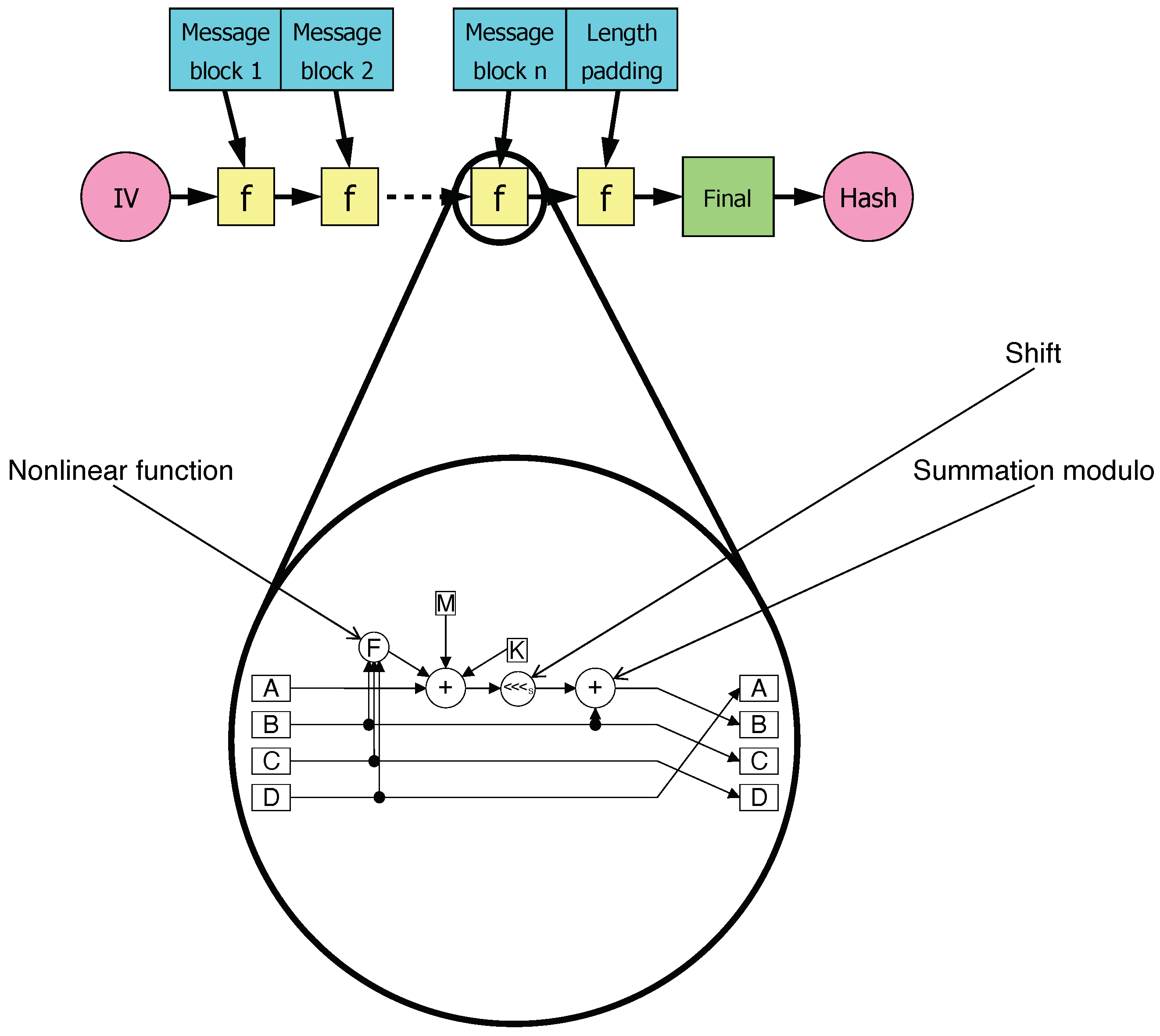
Here, we develop an efficient technique to obtain the solution. Namely, we divide the MD5 hash function into simple operations, which we can easily convert to the MILP or QUBO (Figure 2). Each circle depicts an operation; the white rectangle is a 32 bit number. At a first step, we note that all round functions make the same operations, except a nonlinear function. Therefore, the MILP or QUBO will appear in the similar way. Taking a closer look at the round function, we notice that it consists of the following types of operations: the nonlinear function, addition modulo and shift. Nonlinear functions are used in the MD5 to act on 32 bit numbers separately, and thus, we can find the MILP/QUBO representation for each bit separately. Table 2 gives all nonlinear functions in the MD5 and the respective linear equations for them.
The addition modulo is considered in Section 3.1. For implementing a shift operation (left or right bit rotation), one should just rename the corresponding variables. Let us consider the linear system Φ ( x , y ) = b , where x and y are vectors of variables, and b is a fixed vector of parameters. We need to add a shift operation to x and to leave y unchanged. We denote by x the “shifted” x . By definition, x = x 1 , x 2 , , x N , then x = x s + 1 , x s + 2 , , x N , x 1 , x 2 , , x s in the case of right rotation x = x > > > s and x = x N s , x N s + 1 , , x N , x 1 , x 2 , , x N s 1 in the case of left rotation x = x < < < s . So, the new linear system (after shift) is just the system of simple equations (“reindexing”) Φ ( x , y ) = b Φ x , y = b .
After converting all types of operations in the MILP, we are ready to build it for the whole MD5. Before doing that though, let us shortly revise the definition of MD5. The hash function transforms the 512 bit input message into the hash value. The given message divides into 16 pieces of 32 bit numbers, M i ( i 0 15 ) . In addition, the MD5 has four 32-bit constants, which we define as A 0 , B 0 , C 0 , D 0 , respectively. The calculating of the hash value consists of rounds. The MD5 has 64 rounds. In each round, we calculate some intermediate hash value as follows:
A k = D k 1 , B k = F k B k 1 , C k 1 , D k 1 + A k 1 + M μ ( k ) + K k < < < s k + B k 1 , C k = B k 1 , D k = C k 1
where k 1 64 is the number of rounds, K k and s k are given constant numbers, and μ ( k ) are as follows:
  • μ ( k ) = k 1 ( k 1 16 ) ;
  • μ ( k ) = 5 k 4 ( mod 16 ) ( k 17 32 ) ;
  • μ ( k ) = 3 k + 2 ( mod 16 ) ( k 33 48 ) ;
  • μ ( k ) = 7 k 7 ( mod 16 ) ( k 49 64 ) .
Here F k is one of the nonlinear round functions. Depending on the round number, we have the following:
  • F k ( B , C , D ) = F ( B , C , D ) = ( B C ) ( ! B D ) ( k 1 16 ) ;
  • F k ( B , C , D ) = G ( B , C , D ) = ( B D ) ( C ! D ) ( k 17 32 ) ;
  • F k ( B , C , D ) = H ( B , C , D ) = B C D ( k 33 48 ) ;
  • F k ( B , C , D ) = I ( B , C , D ) = C ( B ! D ) ( k 49 64 ) .
The final hash value of the MD5 is compound of A 64 , B 64 , C 64 , D 64 blocks. Comparing with the notation from the beginning ( H ( x ) = y ) , x is divided into M k blocks, y is the compound of A 64 , B 64 , C 64 , D 64 blocks. More details can be found in [19].
In the Table 2, we specified all nonlinear functions used in MD5. Denote by L k B k 1 , C k 1 , D k 1 , F F k , α k = 0 the linear system of equations for nonlinear operations in the k-th round. This system consists of the linear equation for each bit of B k 1 , C k 1 , D k 1 and is chosen from Table 2 in accordance with the hash function round. Here, F F k is the output number of F k ( B k 1 , C k 1 , D k 1 ) , and α k is a vector variable which denotes all ancilla bits. For example, let us consider the 33-rd round and let all the numbers in the blocks be 2 bit for simplicity’s sake. In the 33-rd round, H ( B , C , D ) is used from Table 2. Then, the linear system L 33 ( B 32 , C 32 , D 32 , F F 33 , α 33 ) = 0 becomes
L 33 ( B 32 , C 32 , D 32 , F F 33 , α 33 ) = 0 : = B 32 , 0 + C 32 , 0 + D 32 , 0 F F 33 , 0 2 α 33 , 0 = 0 B 32 , 1 + C 32 , 1 + D 32 , 1 F F 33 , 1 2 α 33 , 1 = 0
For the addition modulo, we use another notation, Σ ( A , B , , D , R , ξ ) , where A , B , , D are input numbers, R is the output one and ξ is a vector variable of all ancilla bits as in the nonlinear function case. Let us write an explicit formula for Σ in the simple case. For example, consider two 2-bit summands, then Σ is as follows:
Σ ( A , B , R , ξ ) = 0 : = A 0 + B 0 = R 0 + 2 ξ 0 ξ 0 + A 1 + B 1 = R 1 + 2 ξ 1
Using the MD5 round definition and Figure 2, we can write the linear system for one round. Consider the k-th round:
L k B k 1 , C k 1 , D k 1 , F F k , α k = 0 Σ F F k , A k 1 , M μ ( k ) , K k , F M k , ξ k , 1 = 0 Σ F M k < < < s k , B k 1 , B k , ξ k , 2 = 0 A k = D k 1 , C k = B k 1 , D k = C k 1
Combining all of Equation (42), we obtain the MILP for the whole MD5:
L 1 B 0 , C 0 , D 0 , F F 1 , α 1 = 0 Σ F F 1 , A 0 , M μ ( 1 ) , K 1 , F M 1 , ξ 1 , 1 = 0 Σ F M 1 < < < s 1 , B 0 , B 1 , ξ 1 , 2 = 0 A 1 = D 0 , C 1 = B 0 , D 1 = C 0 L k B k 1 , C k 1 , D k 1 , F F k , α k = 0 Σ F F k , A k 1 , M μ ( k ) , K k , F M k , ξ k , 1 = 0 Σ F M k < < < s k , B k 1 , B k , ξ k , 2 = 0 A k = D k 1 , C k = B k 1 , D k = C k 1 L 64 B 63 , C 63 , D 63 , F F 64 , α 64 = 0 Σ F F 64 , A 0 , M μ ( 64 ) , K 64 , F M 64 , ξ 64 , 1 = 0 Σ F M 64 < < < s 64 , B 63 , B 64 , ξ 64 , 2 = 0 A 64 = D 63 , C 64 = B 63 , D 64 = C 63
with the final hash value A 64 , B 64 , C 64 , D 64 .
Now, we calculate the number of binary variables in the MILP of the MD5 hash function. In the zeroth round, we have A 0 , B 0 , C 0 , D 0 and all M i ( i 0 16 ) . They are ( 4 + 16 ) · 32 = 640 bits. Each L k adds F k and α k variables, and F k in each round consists of 32 bits, whereas the number of bits in α k depends on a round. From 1 to 32 rounds, α k has 3 · 32 = 96 bits; from 33 to 48, α k has 32 bits; and from 49 to 64, α k has 64 bits. Finally, all L k have 32 · 64 + 96 · 32 + 32 · 16 + 64 · 16 = 6656 new bits.
Each ξ k , 1 has only 2 bits. One can easily check that because four terms generate 2 carry bits and in the next addition, six terms (4 + 2) also produce 2 carry bits. Taking into account a new bit for F M k and 32 bits, we conclude that Σ adds 3 · 32 = 96 bits in the case of Σ F F k , A k 1 , M μ ( k ) , K k , F M k , ξ k , 1 = 0 . Even easier is with ξ k , 2 , which always has only 1 bit. Therefore, Σ F M k < < < s k , B k 1 , B k , ξ k , 2 = 0 adds 64 bits. In total, all Σ in all rounds generate 10,240 new bits. Taking into consideration A 0 , B 0 , C 0 , D 0 and all M k and excluding A 64 , B 64 , C 64 , D 64 , we get 17,408 bits in total.

3.3. The SHA-256

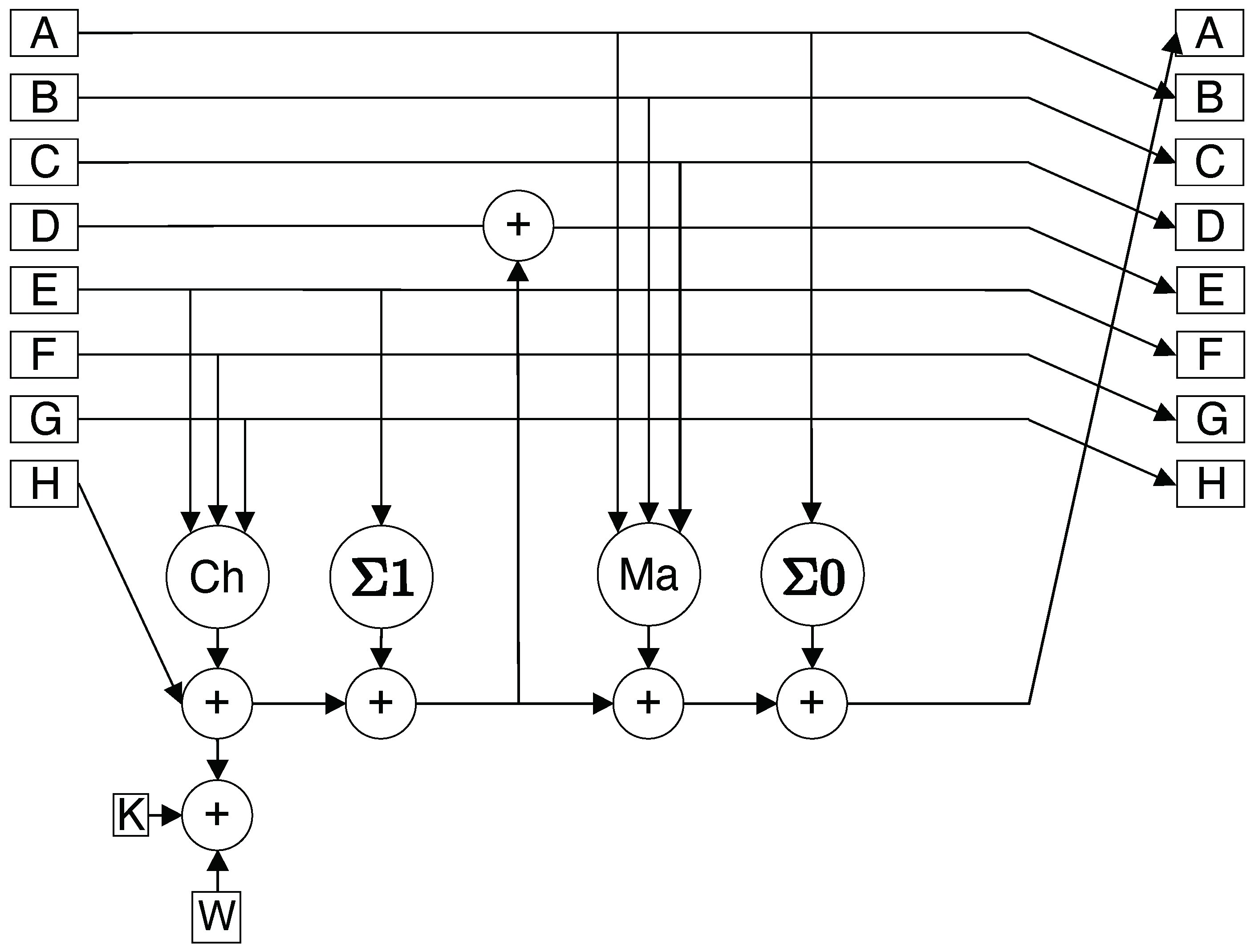
The SHA-256 hash function has a similar structure as well as the MD5 (see Section 3.2) and also has 64 rounds of the similar transformation; see Figure 3. However, there are some differences (for more details, see [20]), namely the following:
  • Each intermediate hash value has 256 bits, which is divided into 8 blocks with 32 bits.
  • A round has four nonlinear functions (Ch, Ma, Σ 1 , Σ 2 ).
  • The input message has 512 bits (16 blocks with 32 bits), and it is extended to 64 blocks using right circular shift and XOR.
Nevertheless, we can convert the SHA256 into MILP (QUBO) as well. In Table 3, we specified all nonlinear functions used in SHA256 and the relevant linear equation. All the MILPs were built by the method from Section 2.1.
The same is with the section about the MD5 (Section 3.2), where we can write the MILP for one round as follows:
L C h ( E k 1 , F k 1 , G k 1 , C H k , α k , 1 ) = 0 , L Σ 1 ( E k 1 , S I G k , 1 , α k , 2 ) = 0 , L Σ 0 ( A k 1 , S I G k , 0 , α k , 3 ) = 0 , L M a ( A k 1 , B k 1 , C k 1 , M A k , α k , 4 ) = 0 , Σ ( H k 1 , S I G k , 1 , C H k , W k , K k , S k , 1 , ξ k , 1 ) = 0 , Σ ( D k 1 , S k , 1 , E k , ξ k , 2 ) = 0 , Σ ( S k , 1 , M A k , A k , ξ k , 3 ) = 0 , B k = A k 1 , C k = B k 1 , D k = C k 1 , F k = E k 1 , G k = F k 1 , H k = G k 1 ,
where L C h , L Σ 1 , L Σ 0 , L M a are linear systems for nonlinear functions from Table 3, Σ is a system for the addition modulo operation, all α and ξ are vectors of binary ancillas for nonlinear and addition transformations, respectively, W k is a block of extended an input message, K k is a given round constant, and A k 1 , B k 1 , C k 1 , D k 1 , E k 1 , F k 1 , G k 1 and H k 1 are blocks of intermediate hash values from the previous round, whereas A k , B k , C k , D k , E k , F k , G k and H k are hash values of the current round.
For extending an input message SHA-256, we use the iterative process, where the first 16 blocks are the same as the input message W k = M k ( k 1 16 ) , and the next W k ( k 17 64 ) is computed as follows:
β k , 0 = ( W k 15 > > > 7 ) ( W k 15 > > > 18 ) ( W k 15 > > 3 )
β k , 1 = ( W k 2 > > > 17 ) ( W k 2 > > > 19 ) ( W k 2 > > 10 )
W k = W k 16 + β k , 0 + W k 7 + β k , 1 mod 2 32
Denote by L ω 0 and L ω 1 the linear system for operation in Equations (45) and (46), respectively. They are built as Σ 0 or Σ 1 in Table 3. γ k , 0 and γ k , 1 are ancilla vector bits for these linear systems. So let us write the full linear system for SHA-256:
W 1 = M 1 , W 2 = M 2 , , W 16 = M 16 , L ω 0 ( W 2 , β 17 , 0 , γ 17 , 0 ) = 0 , L ω 1 ( W 15 , β 17 , 1 , γ 17 , 1 ) = 0 , Σ ( W 1 , β 17 , 0 , W 10 , β 17 , 1 , W 17 , ξ 17 , 0 ) = 0 , L ω 0 ( W 49 , β 64 , 0 , γ 64 , 0 ) = 0 , L ω 1 ( W 62 , β 64 , 1 , γ 64 , 1 ) = 0 , Σ ( W 48 , β 64 , 0 , W 57 , β 64 , 1 , W 64 , ξ 64 , 0 ) = 0 , L C h ( E 0 , F 0 , G 0 , C H 1 , α 1 , 1 ) = 0 , L Σ 1 ( E 0 , S I G 1 , 1 , α 1 , 2 ) = 0 , L Σ 0 ( A 0 , S I G 1 , 0 , α 1 , 3 ) = 0 , L M a ( A 0 , B 0 , C 0 , M A 1 , α 1 , 4 ) = 0 , Σ ( H 0 , S I G 1 , 1 , C H 1 , W 1 , K 1 , S 1 , 1 , ξ 1 , 1 ) = 0 , Σ ( D 0 , S 1 , 1 , E 1 , ξ 1 , 2 ) = 0 , Σ ( S 1 , 1 , M A 1 , A 1 , ξ 1 , 3 ) = 0 , B 1 = A 0 , C 1 = B 0 , D 1 = C 0 , F 1 = E 0 , G 1 = F 0 , H 1 = G 0 , L C h ( E 63 , F 63 , G 63 , C H 64 , α 64 , 1 ) = 0 , L Σ 1 ( E 63 , S I G 64 , 1 , α 64 , 2 ) = 0 , L Σ 0 ( A 63 , S I G 64 , 0 , α 64 , 3 ) = 0 , L M a ( A 63 , B 63 , C 63 , M A 64 , α 64 , 4 ) = 0 , Σ ( H 63 , S I G 64 , 1 , C H 64 , W 64 , K 64 , S 64 , 1 , ξ 64 , 1 ) = 0 , Σ ( D 63 , S 64 , 1 , E 64 , ξ 64 , 2 ) = 0 , Σ ( S 64 , 1 , M A 64 , A 64 , ξ 64 , 3 ) = 0 , B 64 = A 63 , C 64 = B 63 , D 64 = C 63 , F 64 = E 63 , G 64 = F 63 , H 64 = G 63 ,
where union of A 64 , B 64 , C 64 , D 64 , E 64 , F 64 , G 64 , H 64 is final hash value of SHA-256.
In a similar way as in the previous section (Section 3.2), we calculate the number of bits in MILP. For SHA-256, the linear system (Equation (48)) has 46,080 bits.

3.4. The AES

The AES is a symmetric-key cryptography algorithm, meaning that the same key is used for both encrypting and decrypting data [21]. The AES has three different sizes of the key (128, 192 and 256 bits) and the fixed block size of an input message (128 bits). Depending on the key size, the algorithm has a different number of rounds (10, 12 or 14). Then, the protocol decomposes into several parts:
  • KeyExpansion—round keys are derived from the cipher key using the AES key schedule. AES requires a separate 128-bit round key block for each round plus one more.
  • Initial round key addition:
    (a)
    AddRoundKey—each byte of the state is combined with a byte of the round key using bitwise XOR.
  • 9, 11 or 13 rounds:
    (a)
    SubBytes—a non-linear substitution step where each byte is replaced with another according to a lookup table.
    (b)
    ShiftRows—a transposition step where the last three rows of the state are shifted cyclically a certain number of steps.
    (c)
    MixColumns—a linear mixing operation which operates on the columns of the state, combining the four bytes in each column.
    (d)
    AddRoundKey
  • Final round (making 10, 12 or 14 rounds in total):
    (a)
    SubBytes;
    (b)
    ShiftRows;
    (c)
    AddRoundKey.
The first part prepares the key for encoding. Two to four parts are applied sequentially to an input message. An input message has 128 bits and is represented as 4 × 4 with one byte element, termed the state. For instance, let b be the input message with 128 bits or equivalently 16 bytes, and b 0 , b 1 , , b 15 are represented as this two-dimensional array:
b 0 b 4 b 8 b 12 b 1 b 5 b 9 b 13 b 2 b 6 b 10 b 14 b 3 b 7 b 11 b 15
As we mentioned before, we divide the algorithm into smaller parts, transform to linear equations (or QUBO) and merge all parts. Note that the mentioned steps consist of XOR, shifting and operations in Rijndael’s finite field. The first two transformations are considered in Section 3.2. Therefore, let us take a closer look at the last one.

3.4.1. Rijndael’s Finite Field

The several steps are based on the arithmetic in Galois field GF 2 8 = GF ( 2 ) [ x ] / x 8 + x 4 + x 3 + x + 1 . In AES, they use two operations in this field:
  • Inverse operation in GF 2 8 ;
  • Multiplication by 1 , 2 and 3.
The first operation was implemented in Ref. [22]. The calculation of the inverse operation in the GF 2 8 is a hard problem, but it is easy in the GF 2 , where multiplication is the AND operation; therefore, 1 1 = 1 , 0 1 = 0 . (Overall, 0 does not have the inverse element but for definiteness, we put 0 1 = 0 . This agreement is valid for any GF 2 p , p 1 .) In Ref. [22], the authors reduce sequentially the inversion in GF 2 8 into multiplication and inversion in GF 2 4 , then into GF 2 2 and, finally, into GF 2 . For example, the G element in GF 2 8 can be represented as G = γ 1 y + γ 0 with a multiplication modulo, an irreducible polynomial r ( y ) = y 2 + τ y + ν and γ 0 , γ 1 GF 2 4 . Making a similar transformation with step-by-step (more details in [22]) arithmetical operations, only GF 2 is left. So, the given logic gates are enough for making an inversion in GF 2 8 : the XOR, NAND and NOR. All these operations can be transformed into linear equations (QUBO) using our approach from the previous Section 2.1 and Section 2.2. One can see the corresponding linear equation in Table 4. For one byte, it requires 180 gates (XOR, NAND, and NOR) [22]. Each gate is decomposed into one additional equation and two additional bits (z and a).
Multiplications by 1, 2 and 3 in the GF 2 8 are also easy to implement. Multiplying by 1 is exactly the same number ( a × 1 = a ( a GF 2 8 ) . Multiplying by 2 is equivalent to shifting the number left by one, and then XOR’ing the value 0x1B if the high bit was one; otherwise it has to do nothing. Let us build the linear system by steps. x = [ x 0 , x 1 , , x 7 ] is the initial number. In the beginning, we make the shifting and XOR with 0x1B (or 00011011 as the binary number). After that, we obtain z = [ z 0 , z 1 , , z 7 ] . As 0x1B is constant, the XOR gate can be simplified ( a 0 = a , a 1 = a ¯ ). Therefore, after shifting, we have to flip the value if the highest bit of x is equal to 1 and the corresponding bit of 0x1B is also equal to 1. Therefore, the full multiplication is the following linear system:
z 0 = x 7 z 1 = x 7 + x 0 2 a 0 z 2 = x 1 z 3 = x 7 + x 2 2 a 1 z 4 = x 7 + x 3 2 a 2 z 5 = x 4 z 6 = x 5 z 7 = x 6
The equation with two variables can be eliminated because it is just the substitution. So, multiplication by 2 requires 3 additional equations and 6 additional bits. Multiplication by 3 can be considered as follows:
x × 3 = x × ( 2 1 ) = x × 2 x
The XOR operation requires one additional equation and one additional bit per bit. So, multiplication by 3 requires 3 + 8 = 11 additional equations and 22 additional bits.

3.4.2. The Full MILP for the AES

After handling the step with Rijndael’s finite field (Section 3.4.1), other operations are quite easy and consist of only simple gates from Table 4. So we can build the full MILP for AES as in the MD5 case (Section 3.2).
The AES uses a key which can be longer than the message (AES-256 has 256 bits for key and 128 bits for the message). Therefore, one raw message and its cipher are not enough for restoring the full key. However, two known messages (with their ciphers) have a sufficient total length. Therefore, we built two copies of the same linear system (QUBO) for the AES with different known messages (and known) ciphers but linked with the same key. After optimization of these problem, we obtain the key. However, there exists another approach based on the system of quadratic equations; see [23] and the references therein.

3.5. Summary about Cryptography

In Table 5, we calculate the required number of bits in the MILP and qubits in the QUBO, and they are about the same. More precisely, we show the number of variables for the system of linear equations. For inequalities, the numbers of variables differ but remain close. For the AES, the estimates are made with the order of magnitude accuracy.
Unfortunately, the current D-Wave quantum annealer has limited connectivity between the variables. Therefore, before running an experiment at the D-Wave, a user has to embed the original graph into any of the D-Wave’s types of graphs: Chimera or Pegasus. There are methods for embedding an arbitrary graph into these graphs [5,24] which are implemented in the D-Wave software package. We tried to embed our graph from the hash function for one round because the QUBO in each round is the same and connects with a small number of qubits with the QUBO from other rounds. Therefore, embedding the full QUBO based on the merged embeddings is a promising approach since it uses a specific structure of the considered problem. In Table 6, one can see the difference between the number of qubits in the original problem and their number in the problem on the specific graphs of the D-Wave. Unfortunately, we did not implement the corresponding code for the AES yet; this will be a subject of the forthcoming publication.

4. Discussion and Conclusions

We developed the methods for representing any Boolean function as a set of constraints in the mixed-integer linear programming and quadratic unconstrained binary optimization problem with the binary and continuous auxiliary variables. In particular, we investigated the possibility of applications of the developed method for the solution of the cryptographic problems known as a pre-image attack on the hash function, such as the MD5 and SHA256.
The first method represents the Boolean function as one linear equation in the original binary variables and, possibly, ancillary binary variables, which become additional variables of the obtained MILP problem. The method is based on the successive solving of a set of special integer CP problems until the coefficients of the desired linear equation are obtained. Any standard ICP solver may be used; we used the CPLEX solver.
The second method represents the Boolean function as a set of linear inequalities in the original binary variables and one additional continuous variable (representing the value of the function). The method is based on identifying the Boolean function (on n binary variables) with the kind of graphical representation, i.e., the set of 2 n points of the unit cube in R n + 1 . Then, these points are treated as vertices of a convex polyhedron in R n + 1 . To obtain the desired system of linear inequalities, the V-representation of this polyhedron should be converted into H-representation, a set of affine half-spaces of polyhedron facets, i.e., a set of the affine inequalities (one inequality per each affine half-space). For this conversion, we used the LRS application [13], which is a general purpose tool for polyhedron handling.
Note that the first method gives fewer constraints (only one equation per Boolean function) but more ancillary binary variables, while the second method does not require any additional binary variables but instead requires a number of additional linear inequalities. The final decision on the choice between the either first or second method is a trade-off between the number of binary variables and the number of linear constraints in the obtained MILP problem.
Both methods can be used for reformulating the important cryptanalysis problems (pre-imaging of hash functions or breaking symmetric ciphers) based on the Boolean expressions for the MILP problems. Moreover, these methods are applied for formulating the QUBO, deriving it from the given Boolean function (see also [4,5]) and can be used as alternative methods for generating the QUBO with a low number of bits.
Note that for the quantum annealers, the first method is preferable, because most promising quantum annealers proceed along the special type of optimization problems, namely the quadratic unconstrained binary optimization one. The straightforward approach to transform the MILP problem into the QUBO is to convert the linear constraints into the quadratic penalties known as summands of the QUBO problem criterion.

Author Contributions

Conceptualization, A.I.P., V.V.V., V.M.V. and G.B.L.; methodology, A.I.P. and V.V.V.; software, A.I.P.; validation, A.I.P. and V.V.V.; formal analysis, A.I.P. and V.V.V.; investigation, A.I.P. and V.V.V.; resources, A.I.P. and V.V.V.; data curation, A.I.P., V.V.V.; writing—original draft preparation, A.I.P. and V.V.V.; writing—review and editing, A.I.P., V.V.V., V.M.V. and G.B.L.; visualization, A.I.P. and V.V.V.; supervision, V.V.V., V.M.V. and G.B.L.; project administration, V.M.V. and G.B.L.; funding acquisition, V.M.V. and G.B.L. All authors have read and agreed to the published version of the manuscript.

Funding

This research received no external funding.

Institutional Review Board Statement

Not applicable.

Informed Consent Statement

Not applicable.

Data Availability Statement

Our study does not report any data.

Acknowledgments

This work is supported by Terra Quantum AG.

Conflicts of Interest

The authors declare no conflict of interest.

References

  1. Balas, E.; Mazzola, J.B. Nonlinear 0–1 programming: I. Linearization techniques. Math. Program. 1984, 30, 1–21. [Google Scholar] [CrossRef]
  2. Milano, M.; Trick, M. Constraint and integer programming. In Constraint and Integer Programming; Springer: Berlin/Heidelberg, Germany, 2004; pp. 1–31. [Google Scholar]
  3. Hooker, J.N. Logic-based modeling. In Handbook on Modelling for Discrete Optimization; Springer: Berlin/Heidelberg, Germany, 2006; pp. 61–102. [Google Scholar]
  4. Bian, Z.; Chudak, F.; Israel, R.; Lackey, B.; Macready, W.G.; Roy, A. Mapping constrained optimization problems to quantum annealing with application to fault diagnosis. arXiv 2016, arXiv:1603.03111. [Google Scholar] [CrossRef] [Green Version]
  5. Bian, Z.; Chudak, F.; Israel, R.; Lackey, B.; Macready, W.G.; Roy, A. Discrete optimization using quantum annealing on sparse Ising models. Front. Phys. 2014, 2, 56. [Google Scholar] [CrossRef]
  6. Ramos-Calderer, S.; Bellini, E.; Latorre, J.I.; Manzano, M.; Mateu, V. Quantum search for scaled hash function preimages. Quantum Inf. Processing 2021, 20, 180. [Google Scholar] [CrossRef]
  7. Grover, L.K. A fast quantum mechanical algorithm for database search. In Proceedings of the Twenty-Eighth Annual ACM Symposium on Theory of Computing—STOC ’96, New York, NY, USA, 24–26 May 1996. [Google Scholar] [CrossRef] [Green Version]
  8. Rockafellar, R.T. Convex Analysis; Princeton University Press: Princeton, NJ, USA, 1970; p. 452. [Google Scholar]
  9. Avis, D.; Fukuda, K. A pivoting algorithm for convex hulls and vertex enumeration of arrangements and polyhedra. Discret. Comput. Geom. 1992, 8, 295–313. [Google Scholar] [CrossRef]
  10. Fukuda, K. Polyhedral Computation; Department of Mathematics, Institute of Theoretical Computer Science ETH Zurich: Zurich, Switzerland, 2020. [Google Scholar] [CrossRef]
  11. Avis, D.; Fukuda, K.; Picozzi, S. On canonical representations of convex polyhedra. In Mathematical Software; World Scientific: Singapore, 2002; pp. 350–360. [Google Scholar] [CrossRef] [Green Version]
  12. Fukuda, K. cdd, cddplus and cddlib Homepage. Swiss Federal Institute of Technology. 1997. Available online: http://www.inf.ethz.ch/personal/fukudak/cddhome/index.html (accessed on 12 July 2021).
  13. Avis, D. lrs Homepage. McGill University. 2000. Available online: http://cgm.cs.mcgill.ca/~avis/C/lrs.htm (accessed on 12 July 2021).
  14. Rosenberg, I. Reduction of bivalent maximization to the quadratic case. Cah. Cent. D’etudes Rech. Oper. 1975, 17, 71–74. [Google Scholar]
  15. Sasaki, Y.; Aoki, K. Finding Preimages in Full MD5 Faster Than Exhaustive Search. In Advances in Cryptology—EUROCRYPT 2009; Springer: Berlin/Heidelberg, Germany, 2009; pp. 134–152. [Google Scholar] [CrossRef] [Green Version]
  16. Preimage Attack on MD4 Hash Function as a Problem of Parallel Sat-Based Cryptanalysis. Bull. South Ural State Univ. Ser. Comput. Math. Softw. Eng. 2017, 6, 16–27. [CrossRef] [Green Version]
  17. Mironov, I.; Zhang, L. Applications of SAT Solvers to Cryptanalysis of Hash Functions. In Lecture Notes in Computer Science; Springer: Berlin/Heidelberg, Germany, 2006; pp. 102–115. [Google Scholar] [CrossRef] [Green Version]
  18. Dobbertin, H. The First Two Rounds of MD4 are Not One-Way. In Fast Software Encryption; Springer: Berlin/Heidelberg, Germany, 1998; pp. 284–292. [Google Scholar] [CrossRef] [Green Version]
  19. Rivest, R.L. The MD5 Message-Digest Algorithm; RFC, Ed.; RFC 1321; IETF: Fremont, CA, USA, 1992. [Google Scholar] [CrossRef] [Green Version]
  20. Dang, Q.H. Secure Hash Standard; Technical Report, National Institute of Standards and Technology: Gaithersburg, MD, USA, 2015. [Google Scholar] [CrossRef]
  21. Daor, J.; Daemen, J.; Rijmen, V. AES Proposal: Rijndael. 1999. Available online: https://citeseerx.ist.psu.edu/viewdoc/summary?doi=10.1.1.36.640 (accessed on 24 June 2021).
  22. Canright, D. A Very Compact S-Box for AES. In Cryptographic Hardware and Embedded Systems—CHES 2005; Springer: Berlin/Heidelberg, Germany, 2005; pp. 441–455. [Google Scholar] [CrossRef] [Green Version]
  23. Courtois, N.T. General Principles of Algebraic Attacks and New Design Criteria for Cipher Components. In Advanced Encryption Standard—AES; Springer: Berlin/Heidelberg, Germany, 2005; pp. 67–83. [Google Scholar] [CrossRef]
  24. Cai, J.; Macready, W.G.; Roy, A. A practical heuristic for finding graph minors. arXiv 2014, arXiv:1406.2741. [Google Scholar]
Figure 1. Examples of polyhedrons for bi-variant Boolean functions. (a) XOR function. (b) AND function.
Algorithms 15 00033 g001
Figure 2. Dividing MD5 hashing to “simple” problems. The circles denote operations and rectangles indicate integer numbers.
Algorithms 15 00033 g002
Figure 3. Schematic round of SHA-256 hash function.
Algorithms 15 00033 g003
Table 1. Systems of linear inequalities and linear equations for basic Boolean functions.
FormulaSystems of Linear InequalitiesLinear Equation
AND x y = z z x , z y , z x + y 1 , z 0 x + y 2 z a = 0
OR x y = z x z , y z , z x + y , z 1 x + y 2 z + a = 0
XOR x y = z z x + y , z x y , z y x , z 2 x y x + y z 2 a = 0
NOR x y ¯ = z x 1 z , y 1 z , 1 z x + y , z 0 x + y + 2 z a = 1
NAND x y ¯ = z 1 z x , 1 z y , z x + y 2 , 1 z 0 x + y + 2 z a = 2   
Table 2. Nonlinear functions in MD5 hash function.
Boolean FormulaLinear Equation
F ( B , C , D ) ( B C ) ( ¬ B D ) B + 3 C + 2 D 6 F + 2 a 0 3 a 1 + 2 a 2 = 0
G ( B , C , D ) ( B D ) ( C ¬ D ) 3 B + 2 C + D 6 G 3 a 0 + 2 a 1 + 2 a 2 = 0
H ( B , C , D ) B C D B + C + D H 2 a = 0
I ( B , C , D ) C ( B ¬ D ) B + 2 C D 2 I + a 0 4 a 1 = 0
Table 3. Non-linear functions in SHA-256 and relevant linear equations.
Boolean FormulaLinear Equation
Ch ( E , F , G ) = ( E F ) ( ¬ E G ) E + 3 F + 2 G 6 Ch + 2 a 0 3 a 1 + 2 a 2 = 0
Σ 0 A 2 , A 13 , A 22 = A 2 A 13 A 22 A 2 + A 13 A 22 + Σ 0 2 a 0 = 0
Σ 1 A 6 , A 11 , A 25 = A 6 A 11 A 25 A 6 + A 11 A 25 + Σ 1 2 a 0 = 0
Ma ( A , B , C ) = ( A B ) ( A C ) ( B C ) A + B + C 2 Ma a 0 = 0
Table 4. Linear equation for elementary operations (linear equations were found in the previous patent; also there was the method for their generation).
FormulaLinear Equation
AND x y = z E ( x , y , a , z ) { x + y 2 z a = 0 }
OR x y = z E ( x , y , a , z ) { x + y 2 z + a = 0 }
XOR x y = z E ( x , y , a , z ) { x + y z 2 a = 0 }
NOR x y ¯ = z E ¯ ( x , y , a , z ) { x + y + 2 z a = 1 }
NAND x y ¯ = z E ¯ ( x , y , a , z ) { x + y + 2 z a = 2 }
Table 5. Comparing table of problems size.
MD5SHA-256AES-128AES-192AES-256
17,28047,808≈90,000≈2 · 100,000≈2 · 125,000
Table 6. Average number of qubits after embedding for different graphs at D-Wave for one round of hash functions. In the SHA-256 case, D-Wave did not find embedding on the Chimera graph.
MD5SHA-256
Original224415
Chimera943.2-
Pegasus461.11205.9
Publisher’s Note: MDPI stays neutral with regard to jurisdictional claims in published maps and institutional affiliations.