Using Graph Embedding Techniques in Process-Oriented Case-Based Reasoning

Abstract

Similarity-based retrieval of semantic graphs is a core task of Process-Oriented Case-Based Reasoning (POCBR) with applications in real-world scenarios, e.g., in smart manufacturing. The involved similarity computation is usually complex and time-consuming, as it requires some kind of inexact graph matching. To tackle these problems, we present an approach to modeling similarity measures based on embedding semantic graphs via Graph Neural Networks (GNNs). Therefore, we first examine how arbitrary semantic graphs, including node and edge types and their knowledge-rich semantic annotations, can be encoded in a numeric format that is usable by GNNs. Given this, the architecture of two generic graph embedding models from the literature is adapted to enable their usage as a similarity measure for similarity-based retrieval. Thereby, one of the two models is more optimized towards fast similarity prediction, while the other model is optimized towards knowledge-intensive, more expressive predictions. The evaluation examines the quality and performance of these models in preselecting retrieval candidates and in approximating the ground-truth similarities of a graph-matching-based similarity measure for two semantic graph domains. The results show the great potential of the approach for use in a retrieval scenario, either as a preselection model or as an approximation of a graph similarity measure.

1. Introduction

Case-Based Reasoning (CBR) [1,2] is used widely across different domains, e.g., for cooking assistance [3], in smart manufacturing [4], and for data mining support [5]. CBR is a methodology for problem solving where problems and their respective solutions (bundled as cases in a case base) are used to solve upcoming problems (queries). This process relies on similarity computations that are harnessed to find the best-matching case with regard to a given query. It is assumed that the solution of a case can be reused for the given query if the problem of the case is similar to the problem in the query. These core principles are reflected in the CBR cycle [1], which describes four phases of CBR applications: a case is retrieved from the case base according to a given query, reused as a candidate solution, revised to check the fit for the current problem, and retained to be used for further problems. A well-working similarity-based retrieval tool is especially important because, as the first phase, it influences the results of the subsequent phases. A subfield of CBR, which is called Process-Oriented Case-Based Reasoning (POCBR) [6,7,8], focuses on the application of CBR methods and principles in process and workflow management. POCBR particularly aims at managing procedural experiential knowledge, e.g., retrieving workflow models from large repositories [7]. The involved processes are usually represented as semantic graphs [4,5,9], which adds complexity to all involved tasks. For instance, in similarity-based retrieval, the main influential factor on performance is the definition of the similarity measures and the underlying case representation. A simple case representation in the form of feature vectors can be assessed in linear time, while most similarity measures between semantic graphs rely on some form of subgraph isomorphism check, which is computationally expensive, usually with polynomial or exponential complexity [7,10,11]. This example highlights the need for efficient similarity measures between semantic graphs since similarity computations are ubiquitous in POCBR.

One approach to tackle this problem is to reduce the complexity of the semantic graph case representation and to compute similarities with a simplified representation, e.g., by using similarity measures on constructed feature vectors of graphs [12]. However, this reveals a new challenge of identifying important features of semantic graphs, at best, without the need for manual modeling, since it results in increased knowledge acquisition effort [13]. To mitigate this problem and to enable automatic representation learning for semantic graphs, Deep Learning (DL) [14] can be used. A key factor of success for DL is the wide applicability to different types of data, ranging from simple data in the form of one-dimensional feature vectors to more complex data such as graph-structured objects [15,16]. A popular DL method for processing graph-structured data is referred to as graph embedding [17,18]. Graph embedding models are neural networks that learn to represent a graph or its elements in a low-dimensional latent space. The resulting vector representation of embedded graphs enables downstream algorithms to work more efficiently compared to being used on the complex graph structure. Therefore, graph embedding methods are suitable to address the challenge of automatically learning a simplified case representation in POCBR. Further, by adding a component to the neural networks that transforms pairs of embedded graphs to a similarity value, these models can also be directly used as similarity measures.

As a first step towards this goal, our previous work [19] presents the use of an embedding technique in POCBR that accelerates the retrieval process while maintaining almost the same level of retrieval quality as other manually modeled approaches (e.g., [12,20]). The approach uses a general-purpose embedding framework that embeds graph nodes individually, based on graph triplets of two nodes and an edge between them. Thereby, however, only the graph structure is considered in the embedding process, with no integration of the semantic annotations of nodes and edges. Due to this shortcoming, our subsequent approaches [21,22] pursue the idea of using Graph Neural Networks (GNNs) for embedding in POCBR, focusing on the embedding of semantic annotations as well as the graph structure. These publications are extended in this paper to describe graph embedding in POCBR in a broader context. The focus is on integrating embedding methods of semantic graphs as similarity measures in case retrieval. Our main contributions are:

• a comprehensive encoding scheme that enables the integration of semantic graphs with their semantic annotations and structure to be used in GNNs;
• two specialized, adapted GNN architectures for learning similarities between semantic graphs, based on GNNs from the literature [23];
• an evaluation of the GNNs in different retrieval scenarios with regard to performance and quality.

The remainder of the paper is organized as follows: Section 2 presents the foundations of our semantic graph format and the graph matching algorithm for similarity assessment between these semantic graphs. In addition, two variants of similarity-based retrieval are introduced and related work is discussed. In Section 3, we present the architecture of two GNNs, introduced by Li et al. [23], that serve as the basis for our adapted GNNs. Section 4 then elaborates on the encoding procedure for our semantic graph format that transforms the available semantic information into numeric vector space encodings. Furthermore, we present how to adapt the GNNs from Section 3 to be used for predicting pairwise graph similarities. Section 5 describes a system architecture for integrating the GNN-based similarity measures into a POCBR framework and the underlying process of case retrieval. Additionally, Section 6 evaluates the adapted GNNs in the context of different similarity-based retrieval scenarios. Eventually, the conclusions of this paper, together with future research directions, are given in Section 7.

2. Foundations and Related Work

The prerequisite for applying graph embedding techniques in Process-Oriented Case-Based Reasoning (POCBR) is handling the underlying data representation in the form of semantic graphs, which is introduced in Section 2.1. In addition, we explain the similarity assessment procedure for pairs of these semantic graphs (see Section 2.2), which plays a key role in similarity-based retrieval (see Section 2.3). Further, related work is presented to highlight previous and current developments in the use of embedding techniques in Case-Based Reasoning (CBR; see Section 2.4).

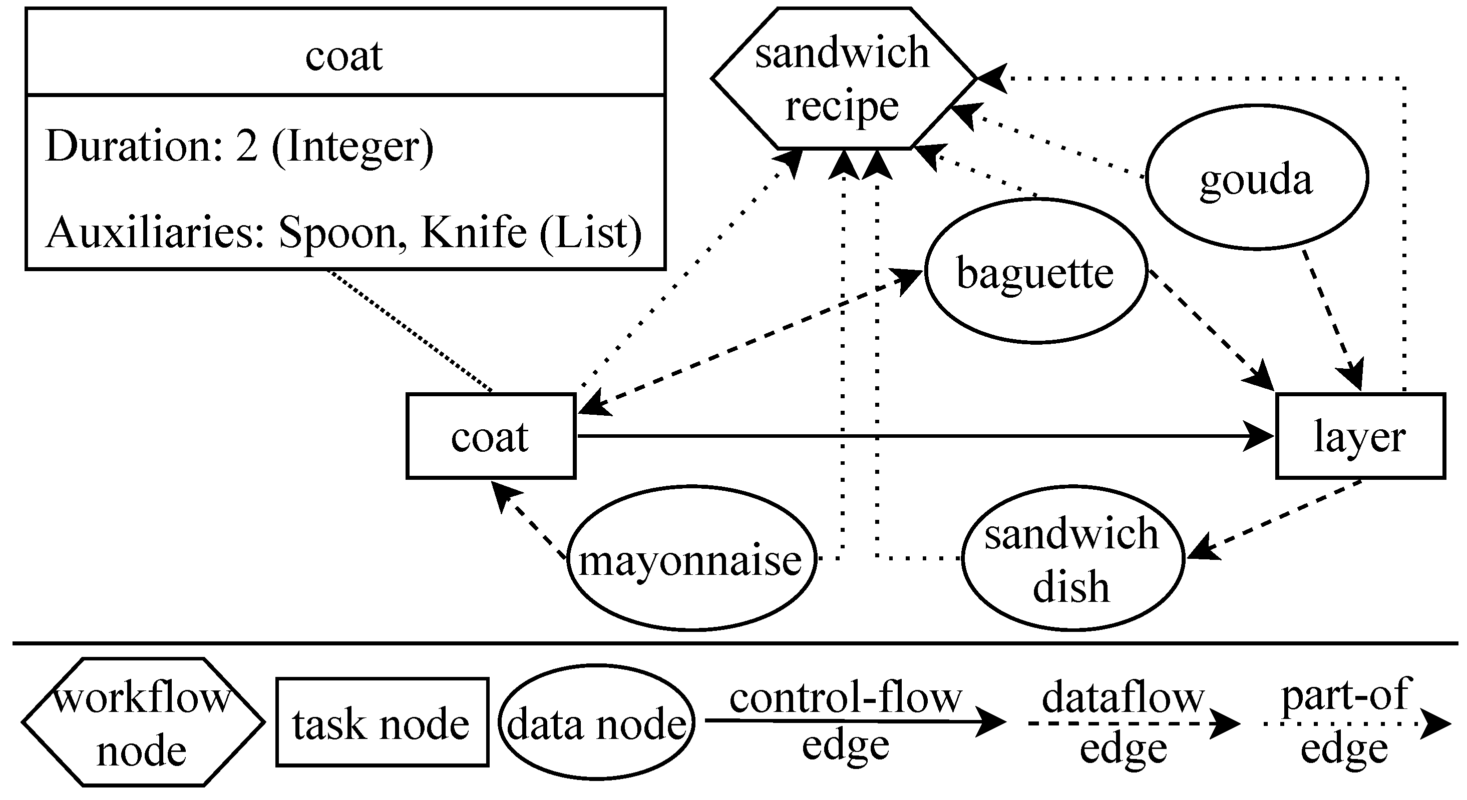
2.1. Semantic Graph Representation

POCBR applications are characterized by a high degree of modeled knowledge. Our semantic graph format allows the integration of semantic knowledge within graph structures. The format is mainly used to model processes and workflows in various domains (e.g., [3,4,5,9]). We represent all cases and queries as semantically annotated directed graphs referred to as NEST graphs, introduced by Bergmann and Gil [7]. More specifically, a NEST graph is a quadruple $G=(N,E,S,T)$ that is composed of a set of nodes N and a set of edges $E\subseteq N\times N$. Each node and each edge has a specific type from $\mathcal{T}$ that is indicated by the function $T:N\cup E\to \mathcal{T}$. Additionally, the function $S:N\cup E\to \mathcal{S}$ assigns a semantic description from $\mathcal{S}$ (semantic metadata language, e.g., an ontology) to nodes and edges. Whereas nodes and edges are used to build the structure of each graph, types and semantic descriptions are additionally used to model semantic information. Hence, each node and each edge can have a semantic description. We denote the number of nodes in a graph as $\left|N\right|\in \mathbb{R}$ and the number of edges as $\left|E\right|\in \mathbb{R}$.

Figure 1 shows a simple example of a NEST graph that represents a cooking recipe for making a sandwich. The mayonnaise–gouda sandwich is prepared by executing the cooking steps coat and layer (task nodes) with the ingredients mayonnaise, baguette, sandwich dish, and gouda (data nodes). All components are linked by edges that indicate relations, e.g., mayonnaise is consumed by coat. Semantic descriptions of task nodes and data nodes are used to further specify semantic information belonging to the recipe components. Figure 1 shows an example of the semantic description of the task node coat. The provided information is used to describe the task more precisely. In this case, a spoon and a knife are needed to execute the task (Auxiliaries) and the estimated time that the task takes is two minutes (Duration). The definition of NEST graphs [7] does not strictly specify the contents of the semantic descriptions in $\mathcal{S}$. To frame the scope of this work regarding semantic descriptions, we refer to the definitions of the POCBR framework ProCAKE [24] since it is widely used in the POCBR literature (e.g., [5,19,21,22,25]). Entries of semantic descriptions in ProCAKE have a certain data type and a content (or value). For instance, the attribute Duration within the semantic description of coat (see Figure 1) has the content 2 and the data type Integer. The available semantic descriptions can be divided into atomic and composite ones, denoted as ${\mathcal{S}}_{\mathrm{atom}}\subset \mathcal{S}$ and ${\mathcal{S}}_{\mathrm{comp}}\subset \mathcal{S}$. The atomic descriptions comprise strings, numerics (integer and double), timestamps, and booleans and represent simple base data. Composite descriptions are more complex and define a structure (or relations) over other composite or atomic data. The composite data comprise attribute–value pairs (dictionaries), lists, and sets. For instance, the semantic description in our example is itself a list of attribute–value pairs, where the attribute Duration is an integer (atomic) and the attribute Auxiliaries is a list (composite). This complexity and flexibility in representation is not easy to handle for Deep Learning (DL) models (see [21,26,27] for more details) and requires specific data encoding methods that will be discussed in our approach.

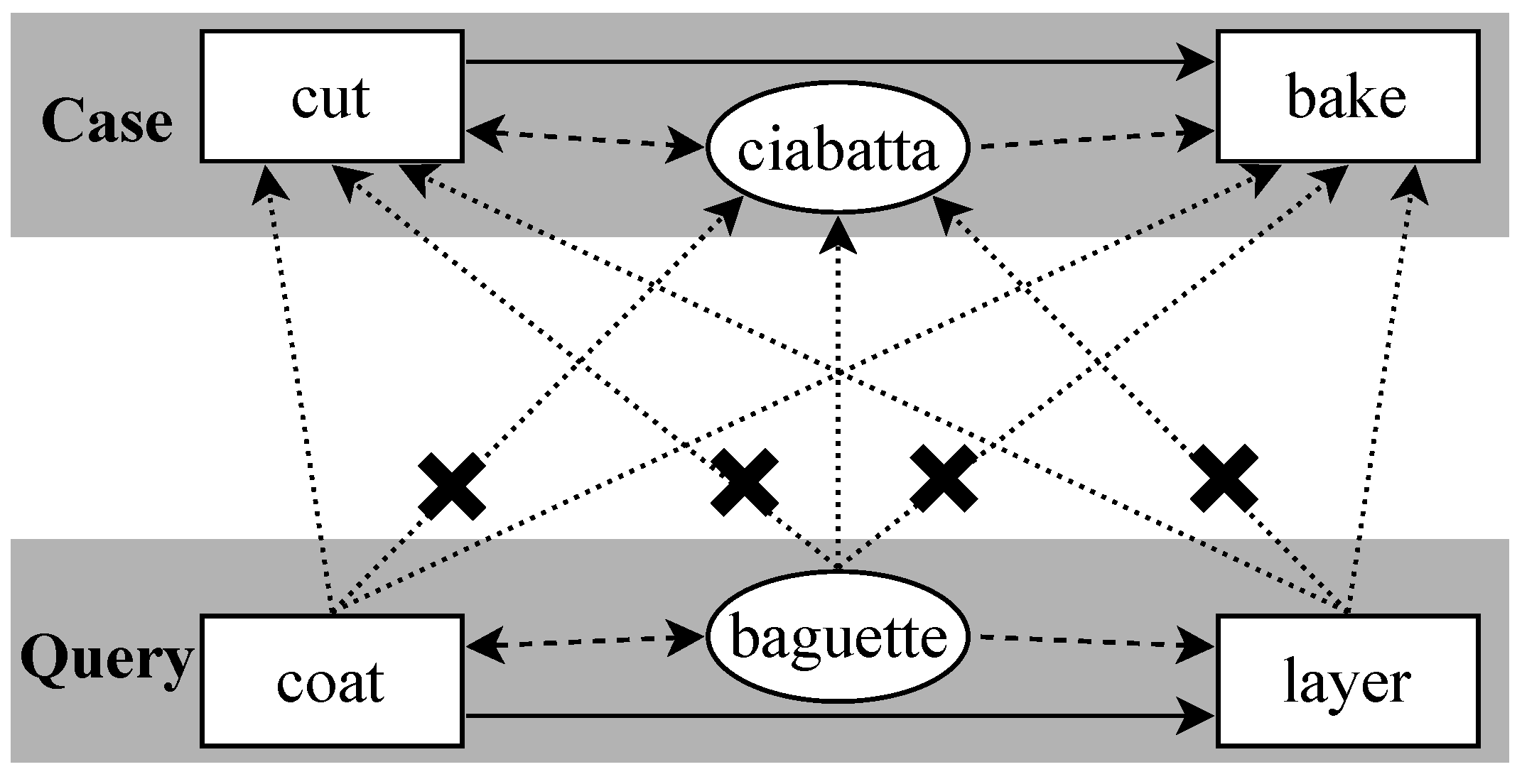
2.2. Similarity Assessment of Semantic Graphs

Determining the similarity between two NEST graphs, i.e., a query graph $\mathit{QG}$ and a case graph $\mathit{CG}$, requires a similarity measure that assesses the structure of nodes and edges as well as the semantic descriptions and types of these components. Bergmann and Gil [7] propose a semantic similarity measure that determines a similarity based on the local–global principle [28]. A global similarity, i.e., the similarity between two graphs, is composed of local similarities, i.e., the pairwise similarities of nodes and edges. The similarity between two nodes with identical types is defined as the similarity of the semantic descriptions of these nodes. The similarity value between two edges with identical types is not only composed of the similarity between the semantic descriptions of these edges, but, in addition, the similarity of the connected nodes is taken into account. For instance, the similarity between the data node baguette from Figure 1 and an arbitrary node from another graph is determined by first checking if their node types are equal. If this is the case, the similarity between both nodes is defined as the similarity between the semantic descriptions of both nodes. The similarity of the node baguette is also part of the similarity assessment of all connected edges, e.g., the dataflow edge to the task node coat. The local–global principle [28] is also harnessed to compute similarities between semantic descriptions of nodes and edges. This means that the global similarity between two semantic descriptions is composed of the local similarities according to the structure of atomic and composite data of these semantic descriptions. When considering the task node coat from Figure 1 as an example, the global similarity between coat and another arbitrary task node with the same structure is composed of the local similarities between the values of Duration and Auxiliaries. The similarity of Auxiliaries is, in turn, dependent on the similarities of individual list items. To make use of the local–global principle for similarity assessment, similarity measures for all components of the semantic descriptions are part of the similarity knowledge associated with the domain. This knowledge usually stems from domain experts and specifically takes into account the type of data [29], e.g., Levenshtein distance for strings and Mean Absolute Error (MAE) for numerics. A common domain model is also required for all graphs and their elements in order to allow the definition of similarity measures between objects that have a comparable structure. The global similarity of the two graphs $\mathit{sim}(\mathit{QG},\mathit{CG})$ is finally calculated by finding an injective partial mapping that maximizes the aggregated local similarities of all pairs of mapped nodes and edges.

The possible node mappings between an excerpt of the graph from Figure 1 and another arbitrary graph are visualized in Figure 2. It highlights the algorithm’s property that nodes and edges with different types are not allowed to be mapped (depicted with bold crosses). That is, the mapping process is constrained according to the types of nodes and edges. Additionally, the figure points out the increase in complexity that comes with the number of nodes and edges, as every node and edge can be mapped onto many other nodes and edges. The complexity of finding a mapping that maximizes the global similarity between a query $\mathit{QG}$ and a single case $\mathit{CG}$ is tackled by utilizing an A* search algorithm, also introduced by Bergmann and Gil [7]. However, A* search is usually time-consuming and can lead to long retrieval times [11,19,21,30]. Therefore, the algorithm features an adjustable parameter for setting the maximum number of partially mapped solutions (called MaxPMS). Adjusting MaxPMS serves as a trade-off between the optimality of the mappings and the time required for finding them, i.e., reducing MaxPMS results in solutions that are not optimal at a lower computation time and vice versa. In most practical applications of the A* search, the search space is very large, which makes it unfeasible to search for a solution to the mapping problem if MaxPMS is unlimited.

2.3. Similarity-Based Retrieval of Semantic Graphs

While the similarity assessment that is shown in Section 2.2 can be used to determine a single similarity between two semantic graphs, it is more common to use it in the retrieve phase of CBR. A retrieval aims to find the most similar cases from a case base $\mathit{CB}$ for a given query $\mathit{QG}$. The most similar cases are determined by computing the pairwise similarity between the query and each case from the case base, before ranking the cases in descending order according to the computed similarities. Many CBR applications only consider the k-most similar cases as result of the retrieval, which is similar to the well-known k-nearest neighbors (kNN) algorithm. Although the retrieval algorithm itself has a computational complexity of $O\left(\right|\mathit{CB}\left|\right)$, the retrieval time is usually dominated by the similarity measure that is used to compare the cases. For instance, measures that perform any kind of inexact subgraph matching (such as the similarity measure introduced in Section 2.2) belong to the class of NP-complete algorithms [7,10,11] and thus have a great impact on performance. To overcome possible performance issues in retrieval situations, the approach of MAC/FAC (“Many are called but few are chosen”), introduced by Forbus et al. [31], can be used. MAC/FAC is a two-staged retrieval approach that aims to decrease the computation time by pre-filtering the case base in the MAC phase to reduce the number of cases that have to be evaluated by a (potentially) computationally complex similarity measure in the subsequent FAC phase. The MAC phase is parameterized by giving a specific similarity measure and a filter size. The approximating similarity measure of the MAC phase usually has low computational complexity and is knowledge-poor, thus introducing the trade-off between quality and performance of the similarity assessment. The filter size is a parameter of the MAC/FAC algorithm that can be used to control how many of the most similar cases according to the MAC similarity measure are transferred to the FAC phase. In general, the results from the MAC stage can be seen as candidates that might be part of the most similar cases regarding the query. With the pre-filtered cases as an input, the FAC phase applies the computationally intensive similarity measure on these candidates. The result is a list of the same length as the filter size that is not guaranteed to contain the most similar cases of the case base according to the query graph. Further truncation to the k-most similar cases can be performed analogously to the standard retrieval. Eventually, MAC/FAC is a trade-off between retrieval quality and retrieval time. The (possibly) decreased quality results from the pre-filtering that might not return the same graphs that a standard retrieval would have returned. The decreased retrieval time is due to a smaller amount of graph pairs that have to be evaluated by the computationally complex, knowledge-intensive similarity measure in the FAC phase. This points out the importance of a well-designed and well-integrated MAC phase as it significantly influences the results of using a MAC/FAC implementation [31,32]. Related MAC/FAC approaches in the context of POCBR use similarity measures that are defined on clustered representations of the case base [20], manually modeled graph features [12], and embeddings of graph triplets [19].

2.4. Related Work

Several approaches have been proposed in CBR research that use DL methods as a key component. There is also strong interest in the combination of DL and CBR methods in the community [26]. To the best of our knowledge, only the work of Klein et al. [19] utilizes a DL-based embedding procedure in the subfield of POCBR. They use a general-purpose embedding framework to learn vector representations in an unsupervised manner, based on the structural properties of semantic graphs, such as the relation between task and data nodes. The approach is evaluated as a similarity measure in retrieval scenarios, where it outperforms other automatically learned approaches and achieves comparable performance to other approaches that are manually modeled. Our approaches in this paper and previous work [21,22] differ from the work of Klein et al. [19] as we not only consider structural graph information for the embedding procedure but also the semantic information of nodes and edges. Outside of POCBR, Mathisen et al. [33] and Amin et al. [34] use embedding techniques and Siamese neural networks in CBR retrieval. The approaches train neural networks to learn similarity measures that are applied in the domains of aquaculture and customer support management, respectively.

The following approaches are related to our work in the broader sense due to their integration of DL components into CBR or vice versa. Most of the approaches automatically learn a similarity measure, similar to our approach. Corchado and Lees [35] integrate a neural network into CBR retrieval and reuse phases, where the network is dynamically retrained during runtime with regard to the current query. The application is used to predict water temperatures along a sea route. Dieterle and Bergmann [36] use neural networks for several tasks within their CBR application that predicts prices of domain names, e.g., for the feature weighting of case attributes. Mathisen et al. [37] investigate methods for learning similarity measures from data. They propose two different strategies with different levels of required manual effort, where the measure with minimal manual modeling outperforms other methods. The application of DL methods in case adaptation is discussed by several other approaches, e.g., [38,39]. These two exemplary approaches pursue the idea of using neural networks for case adaptation by learning to transfer differences between case problems to the respective case solutions. Leake and Ye [40] advance this idea by taking into account that retrieval knowledge and adaptation knowledge are related in CBR. Therefore, they use a specific algorithm to optimize according to both aspects when training neural networks. Furthermore, several papers, such as Gabel and Godehardt [41] and Keane and Kenny [42], tackle a major drawback of DL applications when compared to CBR applications: the reduced explainability. The former approach addresses the problem by projecting DL predictions onto real cases before using them. The latter approach tries to explain the predictions of DL methods with CBR components in a twin-systems approach.

3. Neural Networks for Graph Embedding

For embedding semantic graphs, we rely on Graph Neural Networks (GNNs) that process graph nodes and edges to represent the graph in a low-dimensional latent space. The specific GNN architecture that our approach is based on is presented by Li et al. [23]. Although there are several different GNN architectures presented in the literature (see [27] for an overview of some approaches), that of Li et al. is chosen as a foundation, since they specifically describe and evaluate their approach for the task of similarity-based search, which is closely related to our domain. They describe two GNN variants that are called Graph Embedding Model (GEM) and Graph Matching Network (GMN). Both neural networks work with message-passing between nodes and their features along the edge structure [15,16] as core learning mechanisms. In addition, both neural networks have a Siamese architecture [43,44] that is used to embed two graphs with shared weights and apply a vector similarity measure on the embedding vectors of both graphs. In the following, we introduce the general structure of GEM and GMN (see Section 3.1) and explain the specific components in more detail (see Section 3.2, Section 3.3 and Section 3.4).

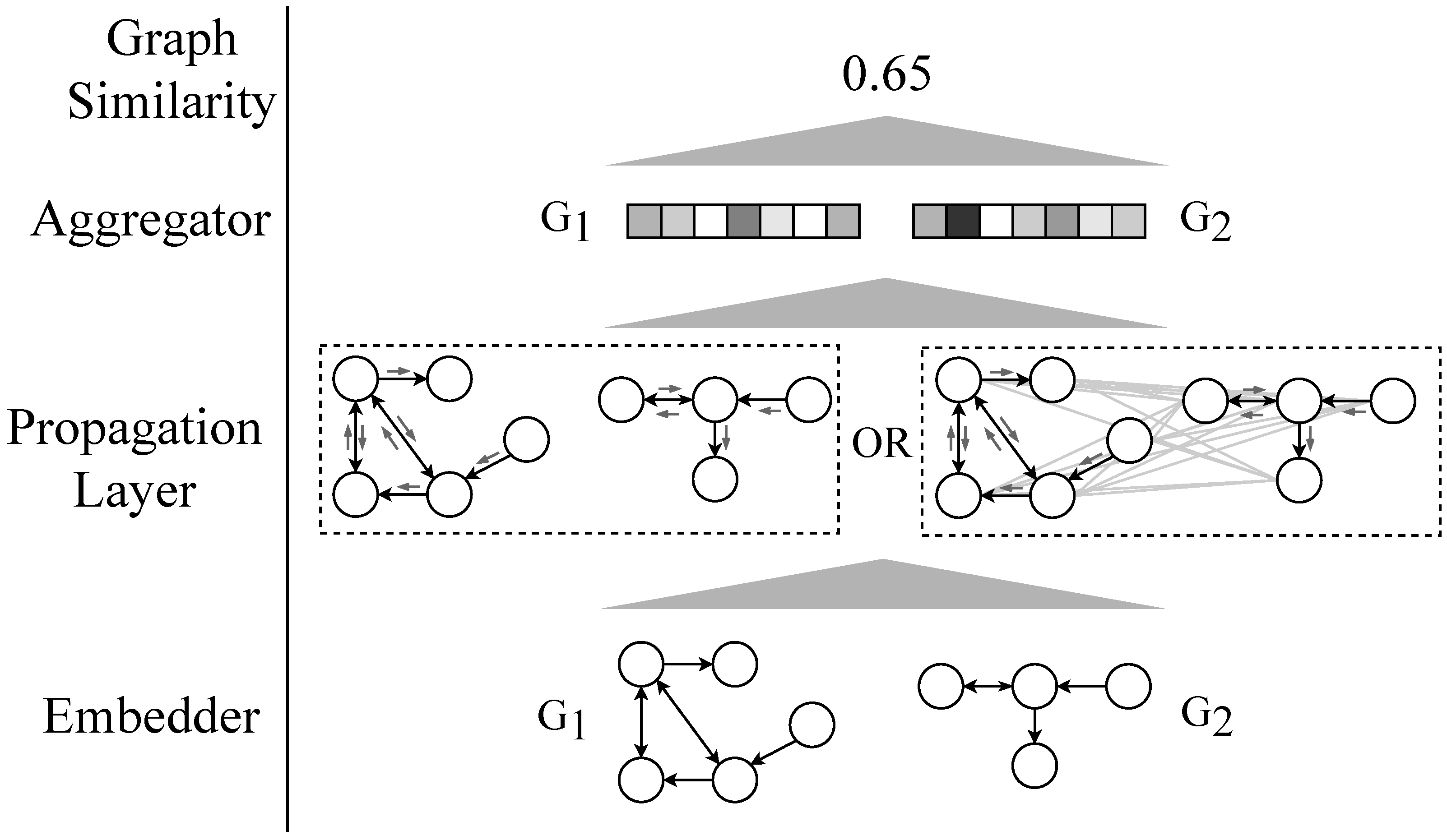
3.1. General Neural Network Structure

The general setup of the neural networks is composed of four main components that are put together in successive order (see Figure 3).

These components are the embedder, the propagation layer, the aggregator, and the graph similarity. The embedder transforms the raw graph input data into an initial vector representation, resulting in a single embedding vector for each node and edge, respectively. During propagation, the vector-based node information is iteratively merged according to the edge structure of the graphs. Thereby, the node embedding vectors are updated via element-wise summations according to the information of all incoming edges and the nodes that are connected via these edges. This captures information about the local neighborhood of each node in its embedding vector. After propagating information for a certain number of rounds, the aggregator combines the embeddings of all nodes from each graph to form a single whole-graph embedding. The final component computes a single scalar similarity value with the embedding vectors of both graphs by utilizing a vector similarity measure such as the cosine similarity. The difference between both models comes from a different propagation strategy. The GEM uses an isolated propagation strategy that only propagates information within a single graph. In contrast, the GMN uses an attention-based cross-graph matching component that propagates information across both graphs in an early state of similarity assessment. In the following, all four components are described more formally and in more detail. The inputs of each neural network are two graph structures $G_1=(N_1,E_1)$ and $G_2=(N_2,E_2)$, although a general graph $G=(N,E)$ with nodes N and edges $E\subseteq N\times N$ is used as a placeholder for components in the Siamese architecture that operate on a single graph.

3.2. Embedder

The embedder computes an initial embedding for all nodes $v,w\in N$ and edges $(v,w)\in E$ to be used in the propagation phase. It is assumed that all nodes and edges have a numeric feature vector that expresses the contained information of a node or an edge. The functions ${\mathit{feat}}_{\mathrm{node}}:N\to {\mathbb{R}}^{l_n}$ and ${\mathit{feat}}_{\mathrm{edge}}:E\to {\mathbb{R}}^{l_e}$ map nodes and edges to their vector encoding in the $l_n$-dimensional and $l_e$-dimensional real space, respectively. For instance, when dealing with NEST graphs, these functions should encode the type and the semantic description of a node or an edge. We discuss the implementation of these functions for our case in Section 4.1 and stick to the generic definition at this point. The embedding procedure can be defined as follows:

$$\begin{array}{cc}\hfill h_v^{\left(0\right)}=& {\mathrm{MLP}}_{\mathrm{node}}\left({\mathit{feat}}_{\mathrm{node}}\left(v\right)\right),\forall v\in N\hfill \\ \hfill h_{v,w}=& {\mathrm{MLP}}_{\mathrm{edge}}\left({\mathit{feat}}_{\mathrm{edge}}(v,w)\right),\forall (v,w)\in E\hfill \end{array}$$

(1)

Each node v is mapped to an embedding vector $h_v^{\left(0\right)}\in {\mathbb{R}}^{l_{nEmb}}$ that is part of an $l_{nEmb}$-dimensional vector space. This embedding vector has the value of transformation step 0 (i.e., the initial embedding), which is depicted by the superscript 0. The mapping is performed by a Multi-Layer Perceptron (MLP) that can be configured in terms of the number of layers, number of hidden neurons, and so on. The edges are mapped in the same fashion. The feature vector of each edge is embedded into $h_{v,w}\in {\mathbb{R}}^{l_{eEmb}}$ by a separate MLP. The resulting edge embedding is located in the $l_{eEmb}$-dimensional vector space. In contrast to node embeddings, edge embeddings do not have an associated transformation step (i.e., superscript 0), because edge representations remain unchanged after the embedding by the embedder. The embeddings of node features are simultaneously used as the initial representation for nodes in the following propagation component (see Section 3.3). They are constantly updated by the neural network, which is indicated by the assigned transformation step, e.g., $h_v^{\left(1\right)}$ after the first update and $h_v^{\left(5\right)}$ after the fifth update. Furthermore, the values of $l_{nEmb}$ and $l_{eEmb}$ (referred to as embedding size) can be used to parameterize the MLPs. The larger the embedding size, the more information can be stored in the particular embedding vector but the more time it takes to compute these vectors.

3.3. Propagation Layer

With the initial embeddings of all nodes and edges, the propagation layer can be applied. This layer differs significantly for GEM and GMN. Therefore, the propagation concept of the GEM will be explained first, and the propagation concept of the GMN afterwards. The propagation layer of the GEM uses edges between nodes to iteratively update the representation of these nodes. In a single one of the K propagation steps, the representation of each node is updated.

$$m_{w,v}={\mathrm{NN}}_{\mathrm{message}}\left([h_v^{\left(k\right)},h_w^{\left(k\right)},h_{v,w}]\right),\forall (v,w)\in E$$

(2)

$m_{w,v}$ is the representation of a single message between nodes. It is composed of the concatenated inputs of the node representation of v, w, and the representation of the edge $e_{v,w}$, transformed by the neural network layer ${\mathrm{NN}}_{\mathrm{message}}$. The type of this layer can be freely chosen but an MLP is recommended by Li et al. [23]. As follows, the message representation $m_{w,v}$ is used to update all node representations from the current state $h_v^{\left(k\right)}$ to the next state $h_v^{(k+1)}$:

$$h_v^{(k+1)}={\mathrm{NN}}_{\mathrm{node}}\left(\left[h_v^{\left(k\right)},\sum _{(w,v)\in E}{m}_{w,v}\right]\right),\forall v\in N$$

(3)

The neural network layer ${\mathrm{NN}}_{\mathrm{node}}$ from Equation (3) takes as inputs a concatenation of the current node state of node v, i.e., $h_v^{\left(k\right)}$, and an aggregation of the message representations of all incoming edges of node v (see Equation (2)). This aggregation can be any commutative element-wise vector operator, e.g., sum, mean, maximum, or minimum. The layer ${\mathrm{NN}}_{\mathrm{node}}$ can either be an MLP or a recurrent layer core such as a Gated Recurrent Unit (GRU) [45] and a Long Short-Term Memory (LSTM) [46]. The GMN approaches propagation from a different point of view to the GEM. Whereas the GEM only considers messages (in the form of edges) within a single graph, the GMN matches nodes from both graphs at an early stage of the similarity assessment.

$$\mathit{att}(h_v^{\left(k\right)},h_w^{\left(k\right)})=\frac{e^{\mathit{vsim}(h_v^{\left(k\right)},h_w^{\left(k\right)})}}{{\displaystyle \sum _{w^{\prime }\in N:N\ni w}{e}^{\mathit{vsim}(h_v^{\left(k\right)},h_{w^{\prime }}^{\left(k\right)})}}}$$

(4)

Equation (4) shows the computation of the function $\mathit{att}$ that computes attention weights using a softmax attention (see [47,48] for a comprehensive explanation of attention in neural networks). In this case, the softmax function can be interpreted as the indication of relevance that the node representation $h_w^{\left(k\right)}$ has for matching with the node representation $h_v^{\left(k\right)}$. The function $\mathit{vsim}$ can be any vector similarity measure, e.g., cosine similarity, that yields a scalar value. To indicate the attention weights of a node from one graph to all nodes of another graph, the descriptor $\mathit{attmat}$ is used. For instance, $\mathit{attmat}(v\in G_1)$ represents a matrix where each row contains the pairwise attention weights (as computed by the function $\mathit{att}$) of the node v from graph $G_1$ to other nodes from graph $G_2$.

$$h_v^{(k+1)}={\mathrm{NN}}_{\mathrm{node}}\left(\left[h_v^{\left(k\right)},\sum _{(w,v)\in E_1}\left(m_{w,v}\right),h_v^{\left(k\right)}\ominus \sum _{w^{\prime }\in N_2}\mathit{attmat}\left(v\right)·h_{w^{\prime }}^{\left(k\right)}\right]\right)$$

(5)

These attention weights are then used in the process of constructing node representations for the next transformation step, i.e., $h_v^{(k+1)}$, by extending the update process of the GEM (see Equation (5)). The extended function ${\mathrm{NN}}_{\mathrm{node}}$ of the GMN takes a third parameter that adds a cross-graph matching component. The cross-graph matching component is made up of the attention weights introduced by Equation (4). The matrix of attention weights of node v, i.e., $\mathit{attmat}\left(v\right)$ is multiplied with the representation vector of all nodes from $G_2$, i.e., $\mathit{attmat}\left(v\right)·h_{w^{\prime }}^{\left(k\right)}$. The resulting vectors are finally aggregated and subtracted element-wise from the node representation of node v. Taking the difference in this case intuitively expresses the distance between node v and the closest neighbor in the other graph [23].

3.4. Aggregator and Graph Similarity

The next step after the propagation layer is the aggregator. The aggregator aggregates all node representations from graph G that result from the K-th iteration of propagation to form a single whole-graph representation $h_G$.

$$h_G={\mathrm{MLP}}_G\left(\sum _{v\in N}\left(\sigma \left({\mathrm{MLP}}_{\mathrm{gate}}\left(h_v^{\left(K\right)}\right)\right)\odot {\mathrm{MLP}}_{\mathrm{state}}\left(h_v^{\left(K\right)}\right)\right)\right)$$

(6)

The aggregation approach in Equation (6) originates from Li et al. [49]. It describes a weighted sum that uses gating vectors as a method to differentiate relevant from irrelevant node representations. At the single node level, the function ${\mathrm{MLP}}_{\mathrm{gate}}$ transforms the node representation $h_v^{\left(K\right)}$ to a gating vector. This gating vector is then activated with the softmax function $\sigma$ (similar to Equation (4)). ${\mathrm{MLP}}_{\mathrm{state}}$ transforms the node representation into a new vector that can then be used in an element-wise multiplication (indicated by the symbol ⊙), resulting in the final single-node representation. The representations of all individual nodes are afterwards combined by an element-wise sum (indicated by the sum symbol Σ) to form a single vector. This single vector finally acts as an input for ${\mathrm{MLP}}_G$, leading to the whole-graph representation $h_G$. $h_G$ is an element of ${\mathbb{R}}^{l_g}$, whereas the vector length $l_g$ can be parameterized and contributes to a trade-off between representation quality (i.e., increased $l_g$) and computation time (i.e., decreased $l_g$).

To obtain a single scalar from the whole-graph representation of the two graphs, represented as the final similarity $\mathit{fsim}(h_{G_1},h_{G_2})$, it is necessary to apply a vector similarity measure on the graph vectors (see Equation (7)).

$$\mathit{fsim}(h_{G_1},h_{G_2})=\mathit{vsim}(h_{G_1},h_{G_2})$$

(7)

Li et al. [23] do not specify the type of vector similarity measure. Common candidates are cosine similarity, dot product, and Euclidean distance. To have a similarity value that is bounded between $[0,1]$, it is recommended to use the cosine similarity in combination with a ReLU activation of ${\mathrm{MLP}}_G$.

4. Neural-Network-Based Semantic Graph Similarity Measure

To apply the Graph Embedding Model (GEM) and the Graph Matching Network (GMN) (introduced in Section 3) as a similarity measure in a retrieval scenario, the neural networks have to be suitable for handling the involved data, i.e., pairs of semantic graphs as input data and a similarity value as output data. To establish a proper integration, we first define an encoding scheme for our semantic graphs that involves encoding the semantic descriptions and types (see Section 4.1). The GEM and the GMN are then adapted to process the encoded semantic graphs and be used as a similarity measure in similarity-based retrieval (see Section 4.2).

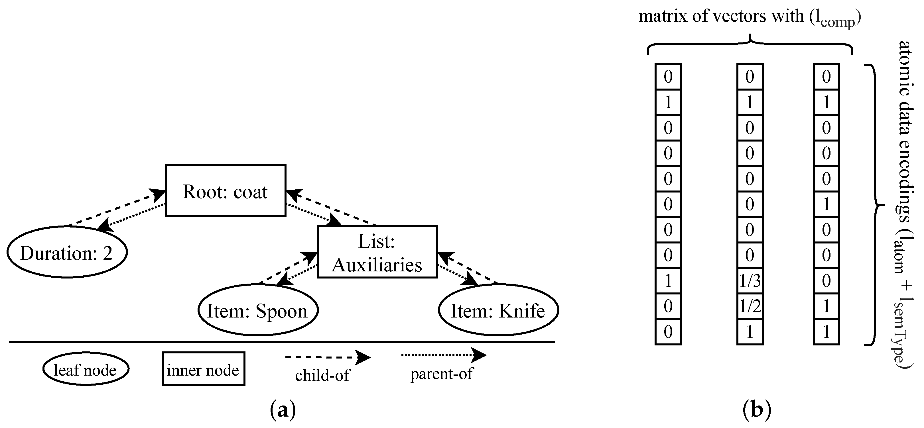
4.1. Encoding Semantic Graphs

An arbitrary NEST graph [7] to encode G has the following four components: the nodes N, the edges E, the semantic descriptions $\mathcal{S}$, and the types $\mathcal{T}$. When looking at the introduced neural networks in Section 3, it is apparent that they are capable of handling the structure of nodes and edges but are not designed to process the rich semantic information and the types of nodes and edges. Li et al. [23] assume nodes and edges to be represented by a feature vector, which is expressed by the functions ${\mathit{feat}}_{\mathrm{node}}:N\to {\mathbb{R}}^{l_n}$ and ${\mathit{feat}}_{\mathrm{edge}}:E\to {\mathbb{R}}^{l_e}$. Since they do not specify how this feature vector is generated, our approach describes specific encoding methods for the types $\mathcal{T}$ (see Section 4.1.1) and the semantic descriptions $\mathcal{S}$ (see Section 4.1.2) in the following. Together with the graph structure that is natively integrated into both Graph Neural Networks (GNNs), this makes it possible to process our semantic graph format.

4.1.1. Encoding Node and Edge Types

The types of nodes and edges (see Section 2.1) are encoded as they are an integral part of semantic graphs. This is also crucial because the types are used to distinguish nodes and edges in terms of similarity. Only nodes and edges with identical types are mapped during similarity computation (see Section 2.2). Each node and each edge has exactly one type, whereas the amount of possible different types, for both nodes and edges, is small. Hence, the types are encoded in the form of one-hot encodings, which is represented by the function ${\mathit{enc}}_{\mathrm{type}}:\mathcal{T}\to {\mathbb{R}}^{l_{\mathrm{type}}}$. According to the NEST definition (see Section 2.1 and [7]), there are, in total, nine different node and edge types, which leads to $l_{\mathrm{type}}=9$. The exemplary graph contains six of these nine different type encodings that are specified by all types in the legend of Figure 1. Nodes or edges with the same type always have the same type of encoding.

4.1.2. Encoding Semantic Descriptions

When encoding semantic descriptions, it is important to describe the underlying structure of these data. As introduced in Section 2.1 and illustrated by the task node coat from Figure 1, semantic descriptions are composed of atomic and composite data with a data type and the respective data content. The possible arrangement of composite types holding atomic types, other nested composite types holding more nested types, and so on can be visualized as a hierarchical tree structure.

Figure 4a shows our semantic description used as a running example in tree form. The depiction distinguishes between leaf nodes (ovals) and inner nodes (rectangles), as well as child-of (dashed lines) and parent-of (dotted lines) relations. The relations between these nodes are defined according to the hierarchical structure of the semantic description, e.g., the item Spoon is a child of the list of Auxiliaries. More formally, the tree representation of the semantic description can be redefined as a graph $G_{\mathrm{sem}}=(N_{\mathrm{comp}}\subseteq {\mathcal{S}}_{\mathrm{comp}},N_{\mathrm{atom}}\subseteq {\mathcal{S}}_{\mathrm{atom}},E_{\mathrm{sem}}\subseteq (N_{\mathrm{comp}}\cup N_{\mathrm{atom}})\times (N_{\mathrm{comp}}\cup N_{\mathrm{atom}}))$ with two sets of nodes and edges between these nodes. The encoding procedure covers the encoding data type and content of entries within the semantic description. This enables the neural network to learn to distinguish different semantic information with regard to both aspects. For instance, in the semantic description of coat, the integer 2 is used as a Duration of type integer. The same number could also be used in a different context (e.g., as the required skill of this task on a 0 to 5 scale), which makes encoding the data type in combination with the content crucial.

We encode the data type as a one-hot vector with the function ${\mathit{enc}}_{\mathrm{semType}}:\mathcal{S}\to {\mathbb{R}}^{l_{\mathrm{semType}}}$. Given a total of five atomic types and three composite types, all vectors have a common vector length of $l_{\mathrm{semType}}=8$ elements. Please note that we are referring to the number of data types of the Process-Oriented Case-Based Reasoning (POCBR) framework ProCAKE [7] with these numbers. In general, the approach is generic and it allows the use of any other framework, as well. This encoding procedure can be extended in certain ways: First, it is possible to encode other atomic or composite data types in the same way. If the atomic types are extended by a data type for timestamps, for instance, it is possible to add a new one-hot encoding for this extension. Second, only encoding the base types, i.e., string, float, list, etc., can be insufficient in certain scenarios where the domain model is very complex (see [4,5] for examples of such domains). The proposed approach can be extended in these cases to use individual one-hot encodings for specific data types in the domain model. For instance, the string entries in the list of Auxiliaries might be defined in a taxonomy, which motivates the use of an individual one-hot vector instead of the generic type vector that is used for all strings.

The second part of encoding semantic descriptions deals with their content. Due to the variety of different types of data, it is difficult to encode these data into a common vector space. This requirement also hinders the use of established existing methods out of the box, e.g., one-hot encoding for string vocabularies [50] or a single scalar value for numerics. We propose to encode the content of one atomic data entry as a single vector with a common vector length $l_{\mathrm{atom}}$ by the function ${\mathit{enc}}_{\mathrm{atom}}:{\mathcal{S}}_{\mathrm{atom}}\to {\mathbb{R}}^{l_{\mathrm{atom}}}$. The elements of this vector are set by a specific encoding method for each data type. Due to space restrictions in this paper, the specific encoding methods cannot be presented in detail. In total, our implementation contains the following specific encoding methods for atomic types: strings that are defined by an enumeration, strings that are defined by a taxonomy, integers, doubles, booleans, and timestamps. Please note that the length of the vector $l_{\mathrm{atom}}$ has to be equal for all encoding procedures to maintain a tensor structure and to allow processing by a neural network.

Encoding composite data mainly focuses on encoding the structure of the atomic data. To be more flexible with defining the architecture of our GNNs, we present two means of encoding composite data that vary in their complexity and require different neural networks for processing: tree encoding to be processed by a GNN and sequence encoding to be processed by a Recurrent Neural Network (RNN; e.g., a Long Short-Term Memory (LSTM) [46] or a Gated Recurrent Unit (GRU) [45]). The tree encoding method preserves the hierarchical structure of the semantic descriptions as modeled in $G_{\mathrm{sem}}=(N_{\mathrm{comp}},N_{\mathrm{atom}},E_{\mathrm{sem}})$. This means that we encode the information provided by both types of nodes, as well as the information provided by the edges. Regarding the nodes from $N_{\mathrm{atom}}$, we can reuse the functions ${\mathit{enc}}_{\mathrm{semType}}$ and ${\mathit{enc}}_{\mathrm{atom}}$ for encoding the data type and the content of the respective node. The content of the nodes of $N_{\mathrm{comp}}$ is usually characterized by the atomic vectors that they are composed of. For instance, the list of Auxiliaries is described by the items in this list. Nevertheless, it can be useful to consider content encodings for composite types in case there is specific information to encode, e.g., the number of list items or their order. We still omit encoding the content and, thus, elements of $N_{\mathrm{comp}}$ are only encoded with the function ${\mathit{enc}}_{\mathrm{semType}}$. The encoding of relations between nodes ($E_{\mathrm{sem}}$) represents the type of relation, i.e., parent-of or child-of. Consequently, it is encoded as a one-hot encoding of length two, given by the function ${\mathit{enc}}_{\mathrm{edge}}:E_{\mathrm{sem}}\to {\mathbb{R}}^2$.

The tree encoding method aims at preserving as much semantic and structural information from the semantic descriptions and the underlying domain model as possible. The drawbacks of its usage are the complex encoding procedure and the need for processing the semantic descriptions with complex GNNs. To mitigate these drawbacks, we provide an alternative encoding method where $G_{\mathrm{sem}}$ is encoded as a sequence of atomic types that can be processed by RNNs. The function ${\mathit{enc}}_{\mathrm{seq}}:N_{\mathrm{comp}}\to {\mathbb{R}}^{l_{\mathrm{comp}} \times l_{\mathrm{atom}} + l_{\mathrm{semType}}}$ is used for this purpose. Each vector in this sequence of atomic data is a concatenation of the data type and the content. Figure 4b shows the encoded sequence of our running example. It contains three atomic encoding vectors that represent the three atomic types of the semantic description given by $N_{\mathrm{atom}}$. Since the sequence encoding does not explicitly model the structure of the semantic description, it is represented by the order of the atomic encoding vectors in the sequence. Therefore, it is necessary to define an ordering scheme for the sequence of each composite type. The only requirement for this ordering scheme is that the atomic vectors are always ordered deterministically. This is important to produce the same encodings for the same semantic descriptions when randomness is present, e.g., for atomic types of an unordered set type. In total, our implementation contains the following specific encoding methods for composite types: attribute–value pairs, lists, and sets.

4.2. Adapted Neural Network Structure

We adjust the architecture of GEM and GMN by Li et al. [23] (see Section 3) for our purpose of similarity-based retrieval in POCBR. The adjusted models are further denoted as Semantic Graph Embedding Model (sGEM) and Semantic Graph Matching Network (sGMN). Resulting from the specific encoding scheme of semantic graphs (see Section 4.1), we present an adjusted embedder (see Section 4.2.1). In addition, the propagation layer (see Section 4.2.2) and the final graph similarity of the GMN (see Section 4.2.3) are also adapted to create a more guided learning process that closely resembles the similarity assessment between semantic graphs. Eventually, we present the loss function that is used for training the neural networks to predict similarities (see Section 4.2.4).

4.2.1. Adapted Embedder

Introduced in Section 3.2, the embedder creates initial embeddings for nodes and edges. Li et al. [23] assume nodes and edges to be represented by a simple feature vector, which is expressed by the functions ${\mathit{feat}}_{\mathrm{node}}:N\to {\mathbb{R}}^{l_n}$ and ${\mathit{feat}}_{\mathrm{edge}}:E\to {\mathbb{R}}^{l_e}$. The challenge for processing our semantic graph format with sGEM and sGMN is how to bridge the gap between our more complex encoded information, i.e., one-hot encoded types and tree- or sequence-encoded semantic descriptions, to the simple one-dimensional feature vector. To achieve this, the adapted embedder embeds the information of semantic descriptions and types separated from each other and concatenates both vectors to form a single feature vector for a node or an edge.

$$\begin{gathered} \begin{array}{cc}\hfill {\mathit{feat}}_{\mathrm{node}}\left(v\right)=& h_v^{\left(0\right)}=\left[h_v^{\mathrm{type}},h_v^{\mathrm{sem}}\right],\forall v\in N\hfill \end{array} \\ {\mathit{feat}}_{\mathrm{edge}}(v,w)=h_{v,w}=\left[h_{v,w}^{\mathrm{type}},h_{v,w}^{\mathrm{sem}}\right],\forall (v,w)\in E \end{gathered}$$

(8)

Equation (8) shows how the embeddings of types, i.e., $h_v^{\mathrm{type}}$ and $h_{v,w}^{\mathrm{type}}$, and semantic descriptions, i.e., $h_v^{\mathrm{sem}}$ and $h_{v,w}^{\mathrm{sem}}$, are combined for each node and edge. This shows how the features of nodes and edges are put together from the available information. In the following, the embedding of types and semantic descriptions is described. The types are embedded as shown in Equation (9):

$$\begin{array}{cc}\hfill h_v^{\mathrm{type}}=& {\mathrm{MLP}}_{\mathrm{ntype}}\left({\mathit{enc}}_{\mathrm{type}}\left(T\left(v\right)\right)\right),\forall v\in N\hfill \\ \hfill h_{v,w}^{\mathrm{type}}=& {\mathrm{MLP}}_{\mathrm{etype}}\left({\mathit{enc}}_{\mathrm{type}}\left(T(v,w)\right)\right),\forall (v,w)\in E\hfill \end{array}$$

(9)

The equation shows the process of embedding node types ($h_v^{\mathrm{type}}$) and edge types ($h_{v,w}^{\mathrm{type}}$). Nodes and edges utilize separate Multi-Layer Perceptrons (MLPs) in this process, i.e., ${\mathrm{MLP}}_{\mathrm{nType}}$ for node types and ${\mathrm{MLP}}_{\mathrm{eType}}$ for edge types, which are applied to the one-hot encoded type vectors. The second part of the combined feature vectors deals with embedding the semantic description of a node or an edge. Since we propose two different encoding methods for semantic descriptions, i.e., a sequence encoding and a tree encoding (see Section 4.1.2), these two encodings are also handled differently.

$$\begin{array}{cc}\hfill h_v^{\mathrm{Sem}}=& {\mathrm{RNN}}_{\mathrm{nSem}}\left({\mathit{enc}}_{\mathrm{seq}}\left(S\left(v\right)\right)\right),\forall v\in N\hfill \\ \hfill h_{v,w}^{\mathrm{sem}}=& {\mathrm{RNN}}_{\mathrm{esem}}\left({\mathit{enc}}_{\mathrm{seq}}\left(S(v,w)\right)\right),\forall (v,w)\in E\hfill \end{array}$$

(10)

Equation (10) shows the embedding of semantic descriptions of nodes ($h_v^{\mathrm{sem}}$) and edges ($h_{v,w}^{\mathrm{sem}}$) that are encoded as a sequence. The sequence structure of the semantic description’s encodings is processed by an unrolled RNN (e.g., [45,46]). An RNN can handle sequences of inputs with different lengths, as they are present in the encodings of semantic descriptions. We use the output state of the last step as the result of the unrolled RNN, which is a single vector. Please note that the sequence contains concatenations of content and data type of semantic description entries (see Section 4.1.2) such that the respective embedding vector captures this information.

When using semantic descriptions that are encoded with the tree encoding method, the embedding step is not implemented with RNNs. Instead, we process the graph $G_{\mathrm{sem}}=(N_{\mathrm{comp}}, N_{\mathrm{atom}}, E_{\mathrm{sem}})$ (introduced in Section 4.1.2) by utilizing a simple GNN that is similar to the GNN architecture that also processes the entire semantic graph. Therefore, the reader can consult the explanations in Section 3 for more details on certain steps. The GNN consists of several trainable components: a component that embeds composite nodes from $N_{\mathrm{comp}}$, i.e., ${\mathrm{NN}}_{\mathrm{comp}}$, a component that embeds atomic nodes from $N_{\mathrm{atom}}$, i.e., ${\mathrm{NN}}_{\mathrm{atom}}$, a component that embeds edges from $E_{\mathrm{sem}}$, i.e., ${\mathrm{NN}}_{\mathrm{edge}}$, a component that performs message propagation, i.e., ${\mathrm{NN}}_{\mathrm{prop}}$, and a component that aggregates the node information to a single graph representation vector, i.e., ${\mathrm{NN}}_{\mathrm{agg}}$. The embedding process is defined as follows:

$$\begin{array}{cc}\hfill {\mathit{htree}}_v^{\left(0\right)}=& {\mathrm{NN}}_{\mathrm{comp}}\left({\mathit{enc}}_{\mathrm{semType}}\left(S\left(v\right)\right)\right),\forall v\in N_{\mathrm{comp}}\hfill \\ \hfill {\mathit{htree}}_v^{\left(0\right)}=& {\mathrm{NN}}_{\mathrm{atom}}\left([{\mathit{enc}}_{\mathrm{semType}}\left(S\left(v\right)\right),{\mathit{enc}}_{\mathrm{atom}}\left(S\left(v\right)\right)]\right),\forall v\in N_{\mathrm{atom}}\hfill \\ \hfill {\mathit{htree}}_{v,w}=& {\mathrm{NN}}_{\mathrm{edge}}\left({\mathit{enc}}_{\mathrm{edge}}(v,w)\right),\forall (v,w)\in E_{\mathrm{sem}}\hfill \end{array}$$

(11)

In the first step (see Equation (11)), all nodes and edges are embedded, which results in the initial embedding vectors ${\mathit{htree}}_v^{\left(0\right)}$ for each node $v\in N_{\mathrm{atom}}\cup N_{\mathrm{comp}}$ and ${\mathit{htree}}_{v,w}$ for each edge $(v,w)\in E_{\mathrm{sem}}$. Thereby, we use the data type and content for embedding nodes from $N_{\mathrm{atom}}$ and only the data type for embedding nodes from $N_{\mathrm{comp}}$. Embedding vectors of edges from $E_{\mathrm{sem}}$ capture the encoded information of the edge representing a child-of or a parent-of relation. The propagation component passes messages between the nodes and updates their state vector accordingly.

$$\begin{array}{cc}\hfill {\mathit{mtree}}_{w,v}=& [{\mathit{htree}}_v^{\left(k\right)},{\mathit{htree}}_w^{\left(k\right)},{\mathit{htree}}_{v,w}],\forall (v,w)\in E_{\mathrm{sem}}\hfill \\ \hfill {\mathit{htree}}_v^{(k+1)}=& {\mathrm{NN}}_{\mathrm{prop}}\left(\left[{\mathit{htree}}_v^{\left(k\right)},\sum _{(w,v)\in E_{\mathrm{sem}}}{\mathit{mtree}}_{w,v}\right]\right),\forall v\in N_{\mathrm{comp}}\cup N_{\mathrm{atom}}\hfill \end{array}$$

(12)

Equation (12) shows the propagation process, where an updated state vector ${\mathit{htree}}_v^{(k+1)}$ is computed for each node $v\in N_{\mathrm{comp}}\cup N_{\mathrm{atom}}$ in each propagation step $k\le K_{\mathrm{tree}}$. This specifies the message-passing step of the GNN, where node information is shared across the edges within the graph. We propose to set the maximum number of propagation steps to 5 based on recommendations from the literature [16,23], i.e., $K_{\mathrm{tree}}=5$.

$${\mathit{htree}}_G={\mathrm{NN}}_{\mathrm{agg}}\left(\sum _{v\in N_{\mathrm{comp}}\cup N_{\mathrm{atom}}}{h}_v^{\left(K_{\mathrm{tree}}\right)}\right)$$

(13)

The final step of the GNN is the aggregation of all node vectors to a single embedding vector that represents the embedded information of the semantic description, i.e., ${\mathit{htree}}_G$. Equation (13) shows the aggregation where the state vectors of all nodes after the final propagation step $K_{\mathrm{tree}}$ are summed up with a commutative element-wise vector function (e.g., sum, mean, etc.) to a single vector. This vector is eventually passed through the neural network ${\mathrm{NN}}_{\mathrm{agg}}$. Please note that the embedding procedure of semantic descriptions in the tree encoding representation is identical for the semantic descriptions of nodes and edges. Thus, the explanations of Equations (11)–(13) hold for nodes as well as edges and ${\mathit{htree}}_G$ is a representative for $h_v^{\mathrm{sem}}$ and $h_{v,w}^{\mathrm{sem}}$. Together with the embedded nodes, this completes $h_v^{\left(0\right)}$ and $h_{v,w}$ from Equation (8).

4.2.2. Constrained Propagation in the Semantic Graph Matching Network

The propagation layer of the GMN uses a cross-graph matching method between the nodes of the two graphs $G_1$ and $G_2$ (see Section 3.3). Each node of $G_1$ is compared with each node of $G_2$ through their softmax-activated cosine vector similarity (ranging between 0 and 1). In this way, information is propagated between the nodes of the two graphs with regard to their pairwise attention. According to the definition of the used graph matching algorithm (see Section 2.2 and [7]), only nodes and edges with the same type are allowed to be matched. That is, the matching process is constrained according to the types of nodes and edges. These constraints can be integrated as an alternative means of message-passing into the cross-graph propagation component of sGMN by only allowing a cosine similarity greater than zero for nodes of the same type. All pairs of nodes with different types are assigned a similarity of 0, representing maximum dissimilarity. Thus, their attention is close to 0, which leads to almost no information propagation between nodes of different types. This extension of GMN’s original cross-graph propagation component can be seen as a form of informed machine learning [51], where prior knowledge is used within a machine learning setup such as our sGMN. See our previous work [22] for a discussion and an application scenario of informed machine learning in POCBR.

4.2.3. Trainable Graph Similarity of Semantic Graph Matching Network

In the definition of GEM and GMN, a vector similarity measure being applied on the vector representations of two graphs $G_1$ and $G_2$, i.e., $\mathit{vsim}(h_{G_1},h_{G_2})$, computes the final similarity value. Such a vector similarity measure is purely syntactic and not trainable regarding patterns in these vectors. Therefore, an MLP-based approach is used to compute the pairwise similarity of two graphs in the sGMN. This emphasizes the nature of the sGMN as a more knowledge-intensive measure (compared to the sGEM) [23] and trades a higher computation time for a better-quality similarity assessment.

$${\mathit{fsim}}_{\mathrm{sGMN}}(h_{G_1},h_{G_2})=\sigma \left({\mathrm{MLP}}_{\mathrm{fsim}}\left([h_{G_1},h_{G_2}]\right)\right)$$

(14)

The approach (see Equation (14)) applies an MLP on the concatenated vector representations of the two graphs. The result of this transformation is lastly activated by a logistic function ($\sigma$) to keep the final similarity in the range of [0,1]. It is important to note that this MLP-based pairwise graph similarity is not symmetrical, which means that, for most graph pairs, ${\mathit{fsim}}_{\mathrm{sGMN}}(h_{G_1},h_{G_2})\ne {\mathit{fsim}}_{\mathrm{sGMN}}(h_{G_2},h_{G_1})$. This is also a property of the graph matching algorithm (see Section 2.2) and other similarity measures in POCBR [29] that is only reflected by this MLP-based graph similarity and not by the cosine vector similarity measure used in the sGEM.

4.2.4. Training and Optimization

Whereas Li et al. [23] assume their training examples to be pairs of graphs that are labeled as similar or dissimilar for training, our training examples are graph pairs with ground-truth similarity values. Hence, each of our training graph pairs is labeled with the ground-truth similarity value, in the range of $[0,1]$. This yields a regression-like problem where the neural network aims to predict similarities that are close to the ground-truth similarities. For this regression problem, the use of a Mean Squared Error (MSE) loss is suitable. When given a batch B of graph pairs $(G_1,G_2)\in B$, the ground-truth similarity of each graph pair $\mathit{sim}(G_1,G_2)\in [0,1]$, and the predicted similarity from one of our models for each graph pair $\mathit{fsim}(h_{G_1},h_{G_2})$, the MSE loss $L_{\mathrm{mse}}$ is computed as follows:

$$L_{\mathrm{mse}}=\frac{{\displaystyle \sum _{(G_1,G_2)\in B}{(\mathit{sim}(G_1,G_2)-\mathit{fsim}(h_{G_1},h_{G_2}))}^2}}{\left|B\right|}$$

(15)

The MSE sums up all squared differences in predicted similarity $\mathit{fsim}(h_{G_1},h_{G_2})$ and labeled similarity $\mathit{sim}(G_1,G_2)$, and then divides this value by the number of all batched training examples to obtain the average deviation. As originally proposed by Li et al. [23], sGEM and sGMN also use the Adam optimizer [52] to optimize the networks’ weights according to the MSE loss value.

5. Application of Semantic Graph Embedding Model and Semantic Graph Matching Network in Similarity-Based Retrieval

The Semantic Graph Embedding Model (sGEM) and the Semantic Graph Matching Network (sGMN) are designed to be used as trainable similarity measures—that is, learning how to predict the similarities of pairs of NEST graphs. The possible application scenarios of sGEM and sGMN in Process-Oriented Case-Based Reasoning (POCBR) are widespread since similarity measures are used in several different tasks, e.g., for retrieving, adapting, or retaining cases [1,2]. We restrict ourselves to the application of the embedding models for retrieving the k-most similar cases according to a query (case retrieval) in this work. Thereby, the integration of the neural networks into a standard retrieval scenario and a MAC/FAC retrieval scenario is examined (see Section 2.3 for an introduction to retrieval and [19,21] for previous work on MAC/FAC in POCBR).

Figure 5 shows the retrieval process, which makes use of two frameworks, i.e., a POCBR framework (e.g., ProCAKE [24]), and a DL Deep Learning (DL) (e.g., TensorFlow [53]). These two frameworks interact while training the neural network in an offline phase (see Section 5.1) and predicting pairwise graph similarities in a retrieval with the neural network. A MAC/FAC retrieval, additionally, performs a subsequent similarity computation with a knowledge-intensive similarity measure (see Section 5.2).

5.1. Offline Training

The offline training phase has the goal of making the neural network learn how to predict similarities between graphs. The phase is initiated by the POCBR framework that encodes the training data and exports them to be used for training. The training data are composed of a case base of semantic graphs, encoded according to the procedure in Section 4.1, and the ground-truth pairwise similarities of these cases. The encoded graphs act as the input data to the neural network and the ground-truth similarities are used as training targets. These target values can be taken from various sources, e.g., computed by the graph similarity measure (see Section 2.2) as in previous work [21,22], or determined by human expert experience. The generated training data are further exported and made available for the training session in the DL framework. The DL framework imports the training data, trains a neural network model (sGEM or sGMN), and exports the trained model. The exported model can be used to resume training at a later point in time, which is helpful to reduce training time in scenarios where dynamic case bases are used (e.g., [5,54]). There are several factors to consider for the training session, e.g., training time and network configuration. Depending on the use case, these settings influence the training success and, eventually, the retrieval quality. Consequently, hyperparameter optimization should be performed for the training process with each case domain. When preparing the trained model to be used in the POCBR framework, it is possible to cache embeddings for all cases of the case base. However, this is only possible with the sGEM since the sGMN has to compute the cross-graph matching component for every pair of the query and the cases (see Section 3.3).

5.2. Retrieval

The data that are utilized during retrieval comprise the case base of NEST graphs, the query NEST graph, and the trained neural network. All cases as well as the query have to be encoded in order to be used with the neural network. Given the encoded graphs, the DL framework is used to predict the similarity of each pair of the query and the cases from the case base. The cached graph representation of each case can be utilized to calculate these similarities if applicable. In this way, only the query graph has to be embedded by the neural network. Hence, the result of the prediction is a list of pairwise similarities that can further be used to determine the nearest neighbors of the query in the case base. A standard retrieval is finished after the k-nearest neighbors are determined. However, sGEM and sGMN are also applicable in a MAC/FAC retrieval (see Section 2.3). The main difference between a standard retrieval and a MAC/FAC retrieval is the use of two consecutive retrieval phases (MAC and FAC phase), where different similarity measures are used. Neural-network-based similarity measures such as the sGEM and the sGMN can be used in both phases, as other approaches demonstrate [19,21]. However, applying a neural network in the MAC phase is usually more reasonable, since the predicted similarities are only an approximation of the true similarities. This can lead to problems with the candidate set, which, on the one hand, might contain cases whose true similarity is lower than the $\mathit{fs}$-threshold or, on the other hand, might not contain cases whose true similarity is higher than the $\mathit{fs}$-threshold. The cases from the possibly wrong set of candidates are then used to compute the final similarity values according to the query. The FAC similarity measure is usually one that is guaranteed to compute the true similarities, e.g., our A* graph matching algorithm (see Section 2.2), since the final similarities directly specify the k-most similar cases, which are returned to the user.

6. Experimental Evaluation

We evaluate the Semantic Graph Embedding Model (sGEM) and the Semantic Graph Matching Network (sGMN) by applying them as similarity measures in standard retrieval and MAC/FAC retrieval scenarios. Thereby, we compare different variants of the embedding models and different retrieval scenarios. The variants are marked with subscripts in our terminology, with a total of six different variants:

sGEM	sGEM used with sequence encoding;
sGEMtree	sGEM used with tree encoding;
sGMN	sGMN used with sequence encoding;
sGMNtree	sGMN used with tree encoding;
sGMNconst	sGMN used with matching constraints;
sGMNtree,const	sGMN used with tree encoding and matching constraints.

As ground-truth similarities for training the neural networks and comparing their predictions, we use similarities computed by the A*-similarity measure by Bergmann and Gil [7] (A*M; see Section 2.2). The ground-truth similarities are computed with a configuration of the measure that uses a very high parameter value for MaxPMS, to allow a good solution to be found in the mapping process. Additionally, we also use this measure with a lower value of MaxPMS in the evaluation to measure the deviations from the ground-truth similarities. This allows us to see how much the computed similarities of A*M deviate from the ground-truth similarities if MaxPMS is reduced. Another evaluated measure is the feature-based measure by Bergmann and Stromer [12] (FBM), which uses a manually modeled feature representation of NEST graphs, specifically designed to be used in combination with a lightweight similarity measure in MAC/FAC retrieval situations. It is included in order to achieve a comparison between automatically learned measures and manually modeled ones, but comparison with this measure is not the main focus. Furthermore, the embedding-based measure of Klein et al. [19] (EBM) is evaluated. It is also designed for MAC/FAC retrieval and utilizes learned graph embeddings and a vector-based similarity (see Section 2.4 for more details). EBM will be the main measure to compare sGEM and sGMN against since it is also automatically learned and embedding-based. We investigate the following hypotheses in two experiments:

Hypothesis 1 (H1).

Using the sGEM variants as MAC similarity measures of a MAC/FAC retrieval leads to improved retrieval results compared to using EBM as a MAC similarity measure;

Hypothesis 2 (H2).

The sGMN variants can approximate the ground-truth graph similarities better than A*M, considering a reduced MaxPMS value such that the retrieval time of both retrievers is comparable.

Each hypothesis refers to a dedicated experiment. The first experiment examines the measures in a MAC/FAC setup, where the focus is placed on the suitability of sGEM as a MAC similarity measure. We focus on evaluating sGEM against the other automatically learned similarity measure, EBM, in H1 as it is, by design, more optimized for performance, which fits the requirements of a MAC similarity measure (see Section 5.2). The second experiment examines the degree to which sGMN is capable of approximating the ground-truth A* similarities. As introduced before, A*M can be configured (by adjusting the MaxPMS parameter) to compute solutions faster with lower quality in return. H2 aims at comparing sGMN to a configuration of A*M with a reduced value of MaxPMS where the deviations from the ground-truth similarities are comparable.

6.1. Experimental Setup

We perform our experiments with an implementation of the presented approach in the Process-Oriented Case-Based Reasoning (POCBR) framework ProCAKE [24] and the Deep Learning (DL) framework TensorFlow [53]. The source code and all supplementary data can be retrieved with the instructions given in the Data Availability Statement on page 22. The neural networks are trained with the help of TensorFlow and the similarity assessment is performed in ProCAKE. Our experiments examine two case bases from different domains that are both represented as semantic NEST graphs. The cooking processes (CB-I) contain 800 sandwich recipes with ingredients and cooking steps [3], split into 660 training cases, 60 validation cases, and 80 test cases. The processes of the data mining domain (CB-II) are built from sample processes that are delivered with RapidMiner (see [5] for more details), split into 509 training cases, 40 validation cases, and 60 test cases. A single training instance is a pair of graphs with the associated similarity value to learn, leading to ${660}^2=435,600$ and ${509}^2=259,081$ training instances, respectively. Thereby, the training case base is used as training input for the neural networks, while the validation case base is used to monitor the training process and to optimize hyperparameter values. Hyperparameter tuning is performed individually per domain with the two base models of sGEM and sGMN. The model variants then use the same hyperparameter settings as the associated base model, e.g., sGEM_tree uses the same hyperparameter configuration as sGEM in the same domain. The training of all models is stopped as soon as the validation loss does not further decrease for two epochs (early stopping).

The metrics that are used to evaluate our approach cover performance and quality. The performance is measured by taking the retrieval time, which is the entire retrieval time including pre-processing of the data if necessary. Since all variants of sGEM and EBM allow for caching of embedding vectors for the case base in an offline phase, these measures only embed the query during the experiments and do not include the caching time in the results. The quality of the results to evaluate $\mathit{RL}\mathrm{eval}$ is measured by comparing them to the ground-truth retrieval results $\mathit{RL}\mathrm{true}$ in terms of Mean Absolute Error (MAE), correctness (see [21,55] for more details), and k-NN quality (see [19,20,21] for more details). The MAE (ranging between 0 and 1) expresses the average similarity error between all pairs of query graph and case graph in $\mathit{RL}\mathrm{true}$ and the same pairs in $\mathit{RL}\mathrm{eval}$. The correctness (ranging between −1 and 1) describes the conformity of the ranking positions of the graph pairs in $\mathit{RL}\mathrm{eval}$ according to $\mathit{RL}\mathrm{true}$. Given two arbitrary graph pairs ${\mathit{GP}}_1=(\mathit{QG},{\mathit{CG}}_1)$ and ${\mathit{GP}}_2=(\mathit{QG},{\mathit{CG}}_2)$, the correctness is decreased if ${\mathit{GP}}_1$ is ranked before ${\mathit{GP}}_2$ in $\mathit{RL}\mathrm{eval}$ although ${\mathit{GP}}_2$ is ranked before ${\mathit{GP}}_1$ in $\mathit{RL}\mathrm{true}$ or vice versa. The k-NN quality (ranging between 0 and 1; see Equation (16)) quantifies the degree to which highly similar cases according to $\mathit{RL}\mathrm{true}$ are present in $\mathit{RL}\mathrm{eval}$.

$$quality(\mathit{QG},{\mathit{RL}}_{\mathrm{true}},{\mathit{RL}}_{\mathrm{eval}})=1-\frac{1}{|{\mathit{RL}}_{\mathrm{true}}|}·\sum _{\mathit{CG}\in {\mathit{RL}}_{\mathrm{true}}\setminus {\mathit{RL}}_{\mathrm{eval}}}\mathit{sim}(\mathit{QG},\mathit{CG})$$

(16)

Therefore, the cases from $\mathit{RL}\mathrm{true}$ are compared with $\mathit{RL}\mathrm{eval}$. Each case from ${\mathit{RL}}_{\mathrm{true}}$ that is missing in $\mathit{RL}\mathrm{eval}$ decreases the quality, with highly relevant cases affecting the quality more strongly than less relevant cases.

The machine that is used for training and testing computations is a PC with an Intel i7 6700 CPU (4 cores, 8 threads), an NVIDIA GTX 3070 GPU, and 48 GB of RAM, running Windows 10. The measures (EBM, all sGEM variants, and all sGMN variants) that require an offline training phase are trained on the GPU with the two training case bases, resulting in two models per measure, i.e., one for each domain. The complete list of training and model parameters can be found in the published source code. To summarize, the models are parameterized such that the GMN models have larger embedding sizes (nodes, edges, graph) than the GEM models and the models for CB-II have larger embedding sizes than the models for CB-I. The average training time is approx. 24 h for the sGMN variants and 8 h for the sGEM variants on average. The inference of all measures is performed only by using the CPU in order to allow a fair comparison. A retrieval is always conducted with a query from the testing case base and with the cases from the training case base. To produce meaningful performance and quality values, the results of the retrieval runs of all query cases from a single domain are averaged.

6.2. Experimental Results

The first experiment aims to answer hypothesis H1 and evaluates the variants of sGEM and sGMN as MAC similarity measures in a scenario of MAC/FAC retrieval. Different combinations of $\mathit{fs}$, i.e., the number of candidates cases of the MAC phase, and k, i.e., the number of retrieval results from the FAC phase, are examined. These values are chosen to be similar to the experiments in previous work [19]. The FAC similarity measure is an A* measure that is used in the same configuration in every retrieval.

Table 1. Evaluation results of the MAC/FAC experiment.

			sGEM		sGEMtree		sGMN		sGMNtree		sGMNconst		sGMNtree,const		FBM		EBM
	fs	k	Quality	Time	Quality	Time	Quality	Time	Quality	Time	Quality	Time	Quality	Time	Quality	Time	Quality	Time
CB-I	5	5	0.508	16	0.511	14	0.489	1051	0.490	2067	0.489	1074	0.489	2169	0.557	510	0.499	17
	50	5	0.613	100	0.600	95	0.522	1137	0.523	2156	0.511	1165	0.505	2263	0.836	611	0.562	100
	10	10	0.520	24	0.536	22	0.502	1061	0.503	2077	0.500	1085	0.505	2180	0.585	522	0.516	25
	80	10	0.623	155	0.609	151	0.581	1195	0.576	2225	0.548	1224	0.575	2330	0.862	671	0.613	158
	25	25	0.545	50	0.567	48	0.534	1088	0.536	2106	0.518	1113	0.534	2208	0.652	554	0.549	53
	100	25	0.606	192	0.593	187	0.646	1240	0.678	2268	0.607	1266	0.676	2373	0.833	714	0.642	195
CB-II	5	5	0.392	66	0.394	84	0.381	2811	0.449	3539	0.399	2729	0.463	3666	0.646	457	0.329	57
	50	5	0.557	866	0.563	895	0.629	3150	0.757	3833	0.671	3016	0.767	3928	0.922	619	0.385	295
	10	10	0.432	113	0.448	123	0.467	2825	0.516	3572	0.457	2785	0.508	3690	0.667	477	0.362	84
	80	10	0.625	1146	0.637	1158	0.745	3406	0.837	4064	0.749	3372	0.853	4197	0.939	744	0.444	430
	25	25	0.506	281	0.511	628	0.550	3004	0.623	3683	0.547	2856	0.628	3793	0.694	533	0.416	198
	100	25	0.683	1371	0.697	1303	0.799	3597	0.872	4234	0.797	3537	0.881	4320	0.907	866	0.500	518

shows the evaluation results, which include the metrics k-NN quality and retrieval time (in milliseconds). Besides the variants of the neural network models, we also evaluate FBM and EBM since these two measures are specifically designed for MAC/FAC applications. The highlighted values represent the maximum quality and minimum time, respectively, for each combination of $\mathit{fs}$ and k.

The results for CB-I show that the two variants of sGEM perform similarly, with similar quality values and retrieval times. The same applies to the quality values of the sGMN variants. The retrieval times of the sGMN variants reveal a negative influence of the variants that use tree encoding, which is likely caused by the more complex embedding process. The sGMN variants and the sGEM variants perform similarly in terms of quality, despite the more expressive embedding process of sGMN. EBM shows quality values that are on par with the values of the sGEM variants. FBM shows the highest quality values across all combinations of $\mathit{fs}$ and k. The retrieval times are higher than those of the sGEM variants and EBM but lower than those of the sGMN variants. The results for CB-II present a similar picture. FBM still outperforms all other measures with regard to quality. However, some sGMN variants, such as sGMN_tree,const, are performing in a similar range. It is also important to note that the sGMN variants with tree encoding are still the slowest measures but outperform all other automatically learned measures for CB-II. The sGMN variants also outperform the sGEM variants for almost all combinations of $\mathit{fs}$ and k, which shows that the variants of sGMN favor retrieval situations with more complex semantic descriptions of task and data nodes, as present in CB-II. The performance of the sGEM and sGMN measures for retrieving graphs from a rather simple domain, such as in CB-I, is respectable but does not consistently surpass the currently available, automatically learned approach of EBM. When only looking at the automatically learned measures in the results of CB-II, i.e., the variants of sGEM, the variants of sGMN, and EBM, sGEM variants are the most suitable for a MAC/FAC scenario since they show a good combination of very low retrieval times and high quality values. The FBM, with its manually modeled similarity measure, still performs best for both case bases, taking into account the combination of quality and time. However, under conditions of strict time requirements, sGEM or EBM can become better suited than FBM. Due to their speed, the measures allow for the performance of a MAC phase with high values of $\mathit{fs}$, which, in turn, produce better overall quality results for the MAC/FAC retrieval. For instance, sGEM can filter with $\mathit{fs}=80$ in less time and with higher ultimate quality than FBM can filter with $\mathit{fs}=10$ to obtain the results for $k=10$. Overall, H1 is partly confirmed due to the similar results of the comparison between sGEM and EBM. None of the different measures clearly outperforms the other. However, sGEM can improve the overall retrieval results under certain conditions ($\mathit{fs}$, k, variant, etc.), which have to be tested for the given scenario.

The second experiment aims to answer hypothesis H2 and examines the degree to which the variants of sGEM and sGMN as well as EBM and FBM can approximate the ground-truth graph similarities (see

Table 2. Evaluation results of the A* approximation experiment.

Domain	CB-I			CB-II
Retriever	MAE	Correctness	Time	MAE	Correctness	Time
sGEM	0.158	0.017	1.3	0.337	0.331	1.1
sGEMtree	0.219	0.053	0.9	0.323	0.310	0.9
sGMN	0.033	0.287	1025.5	0.034	0.583	2697.8
sGMNtree	0.039	0.322	2115.1	0.026	0.724	3508.1
sGMNconst	0.029	0.330	1051.9	0.033	0.583	2643.7
sGMNtree,const	0.037	0.327	2118.3	0.024	0.732	3403.8
FBM	0.193	0.598	482.7	0.199	0.584	335.4
EBM	0.380	0.224	1.2	0.397	0.006	1.1
A*M	0.062	0.669	1265.5	0.041	0.824	3801.8

). We also include a configuration of A*M with an adjusted parameter value of MaxPMS (see Section 2.2) in the experiment. The value for MaxPMS is chosen in such a way that the retrieval time of A*M is similar to that of the sGMN variants. Aligning the retrieval times of A*M and sGMN enables a fair comparison of the resulting MAE and correctness. All reported times are measured in milliseconds.

For CB-I, sGMN_const has the lowest MAE value and A*M has the highest correctness value. The sGEM variants report relatively high MAE values and relatively low values of correctness. The MAE and the correctness values of all sGMN variants are in a similar range, while all outperform the MAE of A*M but are outperformed by A*M in terms of correctness. FBM achieves a high level of correctness but lags in terms of MAE. EBM shows high values of MAE and low values of correctness. When comparing the results of CB-I and CB-II, it becomes apparent that sGMN_tree,const has the lowest MAE and A*M again has the highest value of correctness. The results of the other measures are similar to the results for CB-I. However, it is noticeable that the gap between the sGMN variants and A*M in terms of correctness is smaller. This leads to the assumption that the suitability of sGMN increases with more complex cases. The fact that the variants of sGMN outperform A*M in terms of MAE is even more remarkable when considering that the neural network learns to assess the similarity of graphs without knowing the original algorithmic context, e.g., similarities of semantic descriptions or node and edge mappings. Additionally, this experiment shows that FBM and EBM are not suitable for generating similarities that are close to the ground-truth similarities. The reason for this could be the inadequate processing of semantic annotations and the workflow structure. Thus, we partly accept H2 since the sGMN variants consistently outperform the MAE values of A*M but do not report higher values of correctness.

6.3. Discussion

The two experiments show the suitability of sGEM and sGMN and their different variants in similarity-based retrieval. We would like to discuss some points in particular. First, sGEM and sGMN present inconsistency in the effects that different variants have on different domains. Compared to the base models, these effects can lead to completely different results in different domains. For instance, in the second experiment, sGEM_tree shows a lower MAE than the base model for CB-II but a significantly higher MAE for CB-I. This leads to the need for individual testing of different methods and subsequent hyperparameter tuning. Since the hyperparameters of the models in our experiments are only tuned for the base models, this can certainly lead to further performance improvements. The performance of the sGEM and sGMN variants can further be improved by performing inference on the GPU instead of the CPU (as done in these experiments). Since computations on the GPU are not possible for all other measures, this is a unique characteristic of the neural-network-based models. Furthermore, it is shown that the additional integration of the semantic information of sGEM and sGMN and the usage of Graph Neural Networks (GNNs) can outperform the simple, structural measure, EBM. This confirms the assumption that partly motivated this paper. The effect might be amplified by domains that are even more complex than CB-II, such as argumentation [25] or flexible manufacturing [4]. Additionally, it is shown that sGEM and sGMN, although integrating rich semantic information, are not able to consistently outperform FBM in MAC/FAC retrieval tasks. The usage of manually modeled features and the integration of expert knowledge seems to be superior to automatic learning. Nevertheless, automatically learned measures such as sGEM, sGMN, and EBM still have the advantage of greatly reduced effort when adapting to changes in the similarity definition or the underlying domain models. The overall effort of knowledge acquisition is greatly reduced when using an automatically learned measure. Automatic learning is also helpful when dealing with user-labeled data, since users are usually not capable of labeling cases with concrete similarity values but rather with binary indications, e.g., similar or not similar. The neural networks can learn similarity functions based on these labels with a modified loss function [23,37]. In contrast, this is not straightforward for A*M and FBM as it involves manual configuration effort.

7. Conclusions and Future Work

This paper examines the potential of using two Siamese Graph Neural Networks (GNNs) as similarity measures for retrieving semantic graphs in Process-Oriented CaseBased Reasoning (POCBR). The two presented neural networks, i.e., the Semantic Graph Embedding Model (sGEM) and the Semantic Graph Matching Network (sGMN), can be used in a similarity-based retrieval by predicting the similarities of graph pairs. Therefore, a novel encoding scheme is presented that covers the graph structure, the types of nodes and edges, and their semantic annotations. Given this encoding scheme, sGEM and sGMN are constructed by adapting two neural networks from the literature to fully process pairs of semantic graphs to predict a pairwise similarity value. Setting up the retrieval process with these neural networks in a POCBR framework and a Deep Learning (DL) framework is discussed as well. The experimental evaluation investigates how differently configured variants of sGEM and sGMN perform in similarity-based retrieval. The evaluation covers two domains with different properties, nine different similarity measures, and two different retrieval approaches. The results show the suitability of sGEM and sGMN in the evaluated scenarios. Thereby, sGEM is suitable for a MAC/FAC setup, due to its fast similarity computation and reasonable retrieval quality. Furthermore, sGMN shows great potential in approximating the ground-truth graph similarities.

A focus of future research should be on optimizing the presented approach of a GNN-based retrieval. This optimization ranges from aspects of parameterization to adjustments of the data encoding scheme and the usage of different neural network structures. The neural network structures could be optimized to better process other graph domains, e.g., argument graphs [25], or even other types of complex similarity measures [56]. A structural change could be, for instance, using a differentiable ranking loss function that optimizes according to the ground-truth ordering of the retrieval results (e.g., [57]). Furthermore, the approaches from this paper should be applied to other POCBR tasks, such as case adaptation (e.g., [38]). Since adaptation is usually a knowledge-intensive process, our approaches can help by providing expressive learning capabilities combined with possibilities for domain knowledge integration. Additionally, the neural networks that are used in this work are black boxes and, thus, are not capable of explaining the results they produce. In current research (and also in the CBR community, e.g., [42]), this lack of explainability is tackled in the context of Explainable Artificial Intelligence (XAI). Future research should address this issue by investigating which methods are suitable for increasing the explainability of the presented neural networks.

References

1. Aamodt, A.; Plaza, E. Case-Based Reasoning: Foundational Issues, Methodological Variations, and System Approaches. AI Commun. 1994, 7, 39–59. [Google Scholar] [CrossRef]
2. Richter, M.M.; Weber, R.O. Case-Based Reasoning: A Textbook; Springer: Berlin/Heidelberg, Germany, 2013. [Google Scholar]
3. Müller, G. Workflow Modeling Assistance by Case-Based Reasoning; Springer: Wiesbaden, Germany, 2018. [Google Scholar] [CrossRef]
4. Malburg, L.; Seiger, R.; Bergmann, R.; Weber, B. Using Physical Factory Simulation Models for Business Process Management Research. In Business Process Management Workshops; Del Río Ortega, A., Leopold, H., Santoro, F.M., Eds.; Springer eBook Collection; Springer International Publishing and Imprint Springer: Cham, Switzerland, 2020; Volume 397, pp. 95–107. [Google Scholar] [CrossRef]
5. Zeyen, C.; Malburg, L.; Bergmann, R. Adaptation of Scientific Workflows by Means of Process-Oriented Case-Based Reasoning. In Case-Based Reasoning Research and Development; Bach, K., Marling, C., Eds.; Lecture Notes in Computer Science; Springer: Cham, Switzerland, 2019; Volume 11680, pp. 388–403. [Google Scholar] [CrossRef]
6. Minor, M.; Montani, S.; Recio-García, J.A. Process-Oriented Case-Based Reasoning. Inf. Syst. 2014, 40, 103–105. [Google Scholar] [CrossRef]
7. Bergmann, R.; Gil, Y. Similarity Assessment and Efficient Retrieval of Semantic Workflows. Inf. Syst. 2014, 40, 115–127. [Google Scholar] [CrossRef] [Green Version]
8. Bergmann, R.; Müller, G. Similarity-Based Retrieval and Automatic Adaptation of Semantic Workflows. In Synergies between Knowledge Engineering and Software Engineering; Nalepa, G.J., Baumeister, J., Eds.; Advances in Intelligent Systems and Computing; Springer International Publishing: Cham, Switzerland, 2018; Volume 626, pp. 31–54. [Google Scholar] [CrossRef]
9. Grumbach, L.; Bergmann, R. Using Constraint Satisfaction Problem Solving to Enable Workflow Flexibility by Deviation (Best Technical Paper). In Artificial intelligence XXXIV; Bramer, M.A., Petridis, M., Eds.; Lecture Notes in Computer Science Lecture Notes in Artificial Intelligence; Springer: Cham, Switzerland, 2017; Volume 10630, pp. 3–17. [Google Scholar] [CrossRef]
10. Bunke, H. Recent Developments in Graph Matching. In Proceedings of the 15th International Conference on Pattern Recognition, ICPR’00, Barcelona, Spain, 3–8 September 2000; IEEE Computer Society: Washington, DC, USA, 2000; pp. 2117–2124. [Google Scholar] [CrossRef]
11. Ontañón, S. An overview of distance and similarity functions for structured data. Artif. Intell. Rev. 2020, 53, 5309–5351. [Google Scholar] [CrossRef] [Green Version]
12. Bergmann, R.; Stromer, A. MAC/FAC Retrieval of Semantic Workflows. In Proceedings of the Twenty-Sixth International Florida Artificial Intelligence Research Society Conference, FLAIRS 2013, St. Pete Beach, FL, USA, 22–24 May 2013; Boonthum-Denecke, C., Youngblood, G.M., Eds.; AAAI Press: Palo Alto, CA, USA, 2013. [Google Scholar]
13. Hanney, K.; Keane, M.T. The adaptation knowledge bottleneck: How to ease it by learning from cases. In Case-Based Reasoning Research and Development; Leake, D.B., Plaza, E., Eds.; Lecture Notes in Computer Science; Springer: Berlin/Heidelberg, Germany, 1997; Volume 1266, pp. 359–370. [Google Scholar] [CrossRef]
14. LeCun, Y.; Bengio, Y.; Hinton, G. Deep learning. Nature 2015, 521, 436–444. [Google Scholar] [CrossRef] [PubMed]
15. Scarselli, F.; Gori, M.; Tsoi, A.C.; Hagenbuchner, M.; Monfardini, G. The Graph Neural Network Model. IEEE Trans. Neural Netw. 2009, 20, 61–80. [Google Scholar] [CrossRef] [PubMed] [Green Version]
16. Gilmer, J.; Schoenholz, S.S.; Riley, P.F.; Vinyals, O.; Dahl, G.E. Neural Message Passing for Quantum Chemistry. In Proceedings of the 34th International Conference on Machine Learning, ICML 2017, Sydney, NSW, Australia, 6–11 August 2017; Volume 70, pp. 1263–1272. [Google Scholar]
17. Goyal, P.; Ferrara, E. Graph Embedding Techniques, Applications, and Performance: A Survey. Knowl.-Based Syst. 2018, 151, 78–94. [Google Scholar] [CrossRef] [Green Version]
18. Cai, H.; Zheng, V.W.; Chang, K.C.C. A Comprehensive Survey of Graph Embedding: Problems, Techniques and Applications. IEEE Trans. Knowl. Data Eng. 2018, 30, 1616–1637. [Google Scholar] [CrossRef] [Green Version]
19. Klein, P.; Malburg, L.; Bergmann, R. Learning Workflow Embeddings to Improve the Performance of Similarity-Based Retrieval for Process-Oriented Case-Based Reasoning. In Case-Based Reasoning Research and Development; Bach, K., Marling, C., Eds.; Lecture Notes in Computer Science; Springer: Cham, Switzerland, 2019; Volume 11680, pp. 188–203. [Google Scholar] [CrossRef]
20. Müller, G.; Bergmann, R. A Cluster-Based Approach to Improve Similarity-Based Retrieval for Process-Oriented Case-Based Reasoning. In Proceedings of the ECAI 2014—21st European Conference on Artificial Intelligence—Including Prestigious Applications of Intelligent Systems (PAIS 2014), Prague, Czech Republic, 18–22 August 2014; Schaub, T., Friedrich, G., O’Sullivan, B., Eds.; Frontiers in Artificial Intelligence and Applications. IOS Press: Amsterdam, The Netherlands, 2014; Volume 263, pp. 639–644. [Google Scholar] [CrossRef]
21. Hoffmann, M.; Malburg, L.; Klein, P.; Bergmann, R. Using Siamese Graph Neural Networks for Similarity-Based Retrieval in Process-Oriented Case-Based Reasoning. In Case-Based Reasoning Research and Development; Watson, I., Weber, R., Eds.; Lecture Notes in Computer Science; Springer: Cham, Switzerland, 2020; Volume 12311, pp. 229–244. [Google Scholar] [CrossRef]
22. Hoffmann, M.; Bergmann, R. Informed Machine Learning for Improved Similarity Assessment in Process-Oriented Case-Based Reasoning. arXiv 2021, arXiv:2106.15931. [Google Scholar]
23. Li, Y.; Gu, C.; Dullien, T.; Vinyals, O.; Kohli, P. Graph Matching Networks for Learning the Similarity of Graph Structured Objects. In Proceedings of the 36th International Conference on Machine Learning, ICML 2019, Long Beach, CA, USA, 9–15 June 2019; Volume 97, pp. 3835–3845. [Google Scholar]
24. Bergmann, R.; Grumbach, L.; Malburg, L.; Zeyen, C. ProCAKE: A Process-Oriented Case-Based Reasoning Framework. In Proceedings of the Twenty-seventh International Conference on Case-Based Reasoning (ICCBR 2019), Otzenhausen, Germany, 8–12 September 2019; Volume 2567, pp. 156–161. Available online: CEUR-WS.org (accessed on 13 December 2021).
25. Lenz, M.; Ollinger, S.; Sahitaj, P.; Bergmann, R. Semantic Textual Similarity Measures for Case-Based Retrieval of Argument Graphs. In Case-Based Reasoning Research and Development; Bach, K., Marling, C., Eds.; Lecture Notes in Computer Science; Springer: Cham, Switzerland, 2019; Volume 11680, pp. 219–234. [Google Scholar] [CrossRef]
26. Leake, D.; Crandall, D. On Bringing Case-Based Reasoning Methodology to Deep Learning. In Case-Based Reasoning Research and Development; Watson, I., Weber, R., Eds.; Lecture Notes in Computer Science; Springer: Cham, Switzerland, 2020; Volume 12311, pp. 343–348. [Google Scholar] [CrossRef]
27. Battaglia, P.W.; Hamrick, J.B.; Bapst, V.; Sanchez-Gonzalez, A.; Zambaldi, V.F.; Malinowski, M.; Tacchetti, A.; Raposo, D.; Santoro, A.; Faulkner, R.; et al. Relational inductive biases, deep learning, and graph networks. arXiv 2018, arXiv:1806.01261. [Google Scholar]
28. Richter, M.M. Foundations of Similarity and Utility. In Proceedings of the Twentieth International Florida Artificial Intelligence Research Society Conference, Key West, FL, USA, 7–9 May 2007; Wilson, D., Sutcliffe, G., Eds.; AAAI Press: Palo Alto, CA, USA, 2007; pp. 30–37. [Google Scholar]
29. Bergmann, R. Experience Management: Foundations, Development Methodology, and Internet-Based Applications; Lecture Notes in Computer Science; Springer: Berlin/Heidelberg, Germany, 2002; Volume 2432. [Google Scholar] [CrossRef]
30. Zeyen, C.; Bergmann, R. A*-Based Similarity Assessment of Semantic Graphs. In Case-Based Reasoning Research and Development; Watson, I., Weber, R., Eds.; Lecture Notes in Computer Science; Springer: Cham, Switzerland, 2020; Volume 12311, pp. 17–32. [Google Scholar] [CrossRef]
31. Forbus, K.D.; Gentner, D.; Law, K. MAC/FAC: A Model of Similarity-based Retrieval. Cogn. Sci. 1995, 19, 141–205. [Google Scholar] [CrossRef]
32. Kendall-Morwick, J.; Leake, D. A Study of Two-Phase Retrieval for Process-Oriented Case-Based Reasoning. In Successful Case-based Reasoning Applications-2; Springer: Berlin/Heidelberg, Germany, 2014; pp. 7–27. [Google Scholar]
33. Mathisen, B.M.; Bach, K.; Aamodt, A. Using extended siamese networks to provide decision support in aquaculture operations. Appl. Intell. 2021, 51, 8107–8118. [Google Scholar] [CrossRef]
34. Amin, K.; Lancaster, G.; Kapetanakis, S.; Althoff, K.D.; Dengel, A.; Petridis, M. Advanced Similarity Measures Using Word Embeddings and Siamese Networks in CBR. In Intelligent Systems and Applications; Bi, Y., Bhatia, R., Kapoor, S., Eds.; Advances in Intelligent Systems and Computing; Springer: Cham, Switzerland, 2020; Volume 1038, pp. 449–462. [Google Scholar] [CrossRef]
35. Corchado, J.M.; Lees, B. Adaptation of Cases for Case Based Forecasting with Neural Network Support. In Soft Computing in Case Based Reasoning; Pal, S.K., Ed.; Springer: London, UK, 2001; pp. 293–319. [Google Scholar] [CrossRef] [Green Version]
36. Dieterle, S.; Bergmann, R. A Hybrid CBR-ANN Approach to the Appraisal of Internet Domain Names. In Case-Based Reasoning Research and Development; Lamontagne, L., Plaza, E., Eds.; Lecture Notes in Computer Science; Springer: Cham, Switzerland, 2014; Volume 8765, pp. 95–109. [Google Scholar] [CrossRef]
37. Mathisen, B.M.; Aamodt, A.; Bach, K.; Langseth, H. Learning similarity measures from data. Prog. Artif. Intell. 2020, 9, 129–143. [Google Scholar] [CrossRef] [Green Version]
38. Leake, D.; Ye, X.; Crandall, D. Supporting Case-Based Reasoning with Neural Networks: An Illustration for Case Adaptation. In Proceedings of the AAAI 2021 Spring Symposium on Combining Machine Learning and Knowledge Engineering, Stanford University, Palo Alto, CA, USA, 22–24 March 2021; Martin, A., Hinkelmann, K., Fill, H.G., Gerber, A., Lenat, D., Stolle, R., van Harmelen, F., Eds.; CEUR-WS.org: Palo Alto, CA, USA, 2021. [Google Scholar]
39. Liao, C.K.; Liu, A.; Chao, Y.S. A Machine Learning Approach to Case Adaptation. In Proceedings of the 2018 IEEE First International Conference on Artificial Intelligence and Knowledge Engineering (AIKE), Laguna Hills, CA, USA, 26–28 September 2018; pp. 106–109. [Google Scholar] [CrossRef]
40. Leake, D.; Ye, X. Harmonizing Case Retrieval and Adaptation with Alternating Optimization. In Case-Based Reasoning Research and Development; Sánchez-Ruiz, A.A., Floyd, M.W., Eds.; Lecture Notes in Computer Science; Springer International Publishing: Cham, Switzerland, 2021; Volume 12877, pp. 125–139. [Google Scholar] [CrossRef]
41. Gabel, T.; Godehardt, E. Top-Down Induction of Similarity Measures Using Similarity Clouds. In Case-Based Reasoning Research and Development; Hüllermeier, E., Ed.; Lecture Notes in Computer Science; Springer: Cham, Switzerland, 2015; Volume 9343, pp. 149–164. [Google Scholar] [CrossRef]
42. Keane, M.T.; Kenny, E.M. How Case-Based Reasoning Explains Neural Networks: A Theoretical Analysis of XAI Using Post-Hoc Explanation-by-Example from a Survey of ANN-CBR Twin-Systems. In Case-Based Reasoning Research and Development; Bach, K., Marling, C., Eds.; Lecture Notes in Computer Science; Springer: Cham, Switzerland, 2019; Volume 11680, pp. 155–171. [Google Scholar] [CrossRef]
43. Bromley, J.; Bentz, J.W.; Bottou, L.; Guyon, I.; LeCun, Y.; Moore, C.; Säckinger, E.; Shah, R. Signature Verification Using A “Siamese” Time Delay Neural Network. Int. J. Pattern Recognit. Artif. Intell. 1993, 7, 669–688. [Google Scholar] [CrossRef] [Green Version]
44. Baldi, P.; Chauvin, Y. Neural Networks for Fingerprint Recognition. Neural Comput. 1993, 5, 402–418. [Google Scholar] [CrossRef]
45. Cho, K.; van Merrienboer, B.; Gulcehre, C.; Bahdanau, D.; Bougares, F.; Schwenk, H.; Bengio, Y. Learning Phrase Representations using RNN Encoder–Decoder for Statistical Machine Translation. In Proceedings of the 2014 Conference on Empirical Methods in Natural Language Processing (EMNLP), Doha, Qatar, 25–29 October 2014; Alessandro Moschitti, Q.C.R.I., Bo Pang, G., Walter Daelemans, U.o.A., Eds.; Association for Computational Linguistics: Stroudsburg, PA, USA, 2014; pp. 1724–1734. [Google Scholar] [CrossRef]
46. Hochreiter, S.; Schmidhuber, J. Long Short-Term Memory. Neural Comput. 1997, 9, 1735–1780. [Google Scholar] [CrossRef] [PubMed]
47. Bahdanau, D.; Cho, K.; Bengio, Y. Neural Machine Translation by Jointly Learning to Align and Translate. In Proceedings of the 3rd International Conference on Learning Representations, ICLR 2015, San Diego, CA, USA, 7–9 May 2015. [Google Scholar]
48. Vaswani, A.; Shazeer, N.; Parmar, N.; Uszkoreit, J.; Jones, L.; Gomez, A.N.; Kaiser, L.; Polosukhin, I. Attention is All you Need. In Proceedings of the Advances in Neural Information Processing Systems 30: Annual Conference on Neural Information Processing Systems 2017, Long Beach, CA, USA, 4–9 December 2017; Guyon, I., von Luxburg, U., Bengio, S., Wallach, H.M., Fergus, R., Vishwanathan, S.V.N., Garnett, R., Eds.; Curran Associates, Inc.: Red Hook, NY, USA, 2017; pp. 5998–6008. [Google Scholar]
49. Li, Y.; Tarlow, D.; Brockschmidt, M.; Zemel, R.S. Gated Graph Sequence Neural Networks. In Proceedings of the 4th International Conference on Learning Representations, ICLR 2016, San Juan, Puerto Rico, 2–4 May 2016. [Google Scholar]
50. Mikolov, T.; Chen, K.; Corrado, G.; Dean, J. Efficient Estimation of Word Representations in Vector Space. In Proceedings of the 1st International Conference on Learning Representations, ICLR 2013, Scottsdale, AZ, USA, 2–4 May 2013. [Google Scholar]
51. von Rueden, L.; Mayer, S.; Beckh, K.; Georgiev, B.; Giesselbach, S.; Heese, R.; Kirsch, B.; Walczak, M.; Pfrommer, J.; Pick, A.; et al. Informed Machine Learning—A Taxonomy and Survey of Integrating Prior Knowledge into Learning Systems. IEEE Trans. Knowl. Data Eng. 2021, 18, 19–20. [Google Scholar] [CrossRef]
52. Kingma, D.P.; Ba, J. Adam: A Method for Stochastic Optimization. In Proceedings of the 3rd International Conference on Learning Representations, ICLR 2015, San Diego, CA, USA, 7–9 May 2015. [Google Scholar]
53. Abadi, M.; Barham, P.; Chen, J.; Chen, Z.; Davis, A.; Dean, J.; Devin, M.; Ghemawat, S.; Irving, G.; Isard, M.; et al. TensorFlow: A System for Large-Scale Machine Learning. In Proceedings of the 12th USENIX Conference on Operating Systems Design and Implementation, OSDI’16, Savannah, GA, USA, 2–4 November 2016; USENIX Association: Berkeley, CA, USA, 2016; pp. 265–283. [Google Scholar]
54. Stram, R.; Reuss, P.; Althoff, K.D. Dynamic Case Bases and the Asymmetrical Weighted One-Mode Projection. In Case-Based Reasoning Research and Development; Cox, M.T., Funk, P., Begum, S., Eds.; Lecture Notes in Computer Science; Springer: Cham, Switzerland, 2018; Volume 11156, pp. 385–398. [Google Scholar] [CrossRef]
55. Cheng, W.; Rademaker, M.; de Baets, B.; Hüllermeier, E. Predicting Partial Orders: Ranking with Abstention. In Cellular automata; Bandini, S., Manzoni, S., Umeo, H., Vizzari, G., Eds.; Lecture Notes in Computer Science; Springer: Berlin, Germany, 2010; Volume 6321, pp. 215–230. [Google Scholar] [CrossRef] [Green Version]
56. Mougouie, B.; Bergmann, R. Similarity Assessment for Generalized Cases by Optimization Methods. In Advances in Case-Based Reasoning; Craw, S., Preece, A., Eds.; Lecture Notes in Computer Science; Springer: Berlin/Heidelberg, Germany, 2002; Volume 2416, pp. 249–263. [Google Scholar] [CrossRef] [Green Version]
57. Liu, T.Y. Learning to Rank for Information Retrieval; Springer: Berlin/Heidelberg, Germany, 2011. [Google Scholar] [CrossRef]
Figure 1. Exemplary cooking recipe represented as a NEST graph.
Algorithms 15 00027 g001
Figure 2. Mapping procedure of nodes with illegal mappings.
Algorithms 15 00027 g002
Figure 3. Graph Embedding Model (GEM; left branch) and Graph Matching Network (GMN; right branch) (derived from [23]).
Algorithms 15 00027 g003
Figure 4. Encoding of composite types: (a) Tree encoding (b) Sequence encoding.
Algorithms 15 00027 g004
Figure 5. Retrieval by using a neural-network-based similarity measure.
Algorithms 15 00027 g005