
meta.shrinkage: An R Package for Meta-Analyses for Simultaneously Estimating Individual Means


Abstract
:1. Introduction
2. Background
2.1. Meta-Analysis
2.2. Improved Estimation of Individual Means
3. R Package meta.shrinkage
- y: a vector for s;
- s: a vector for s.
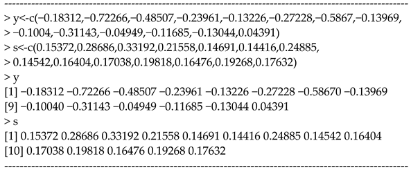
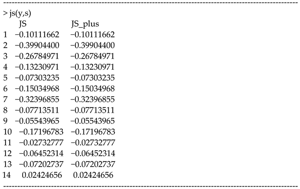
3.1. James–Stein Estimator
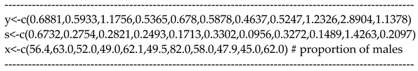
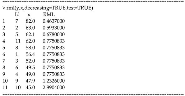
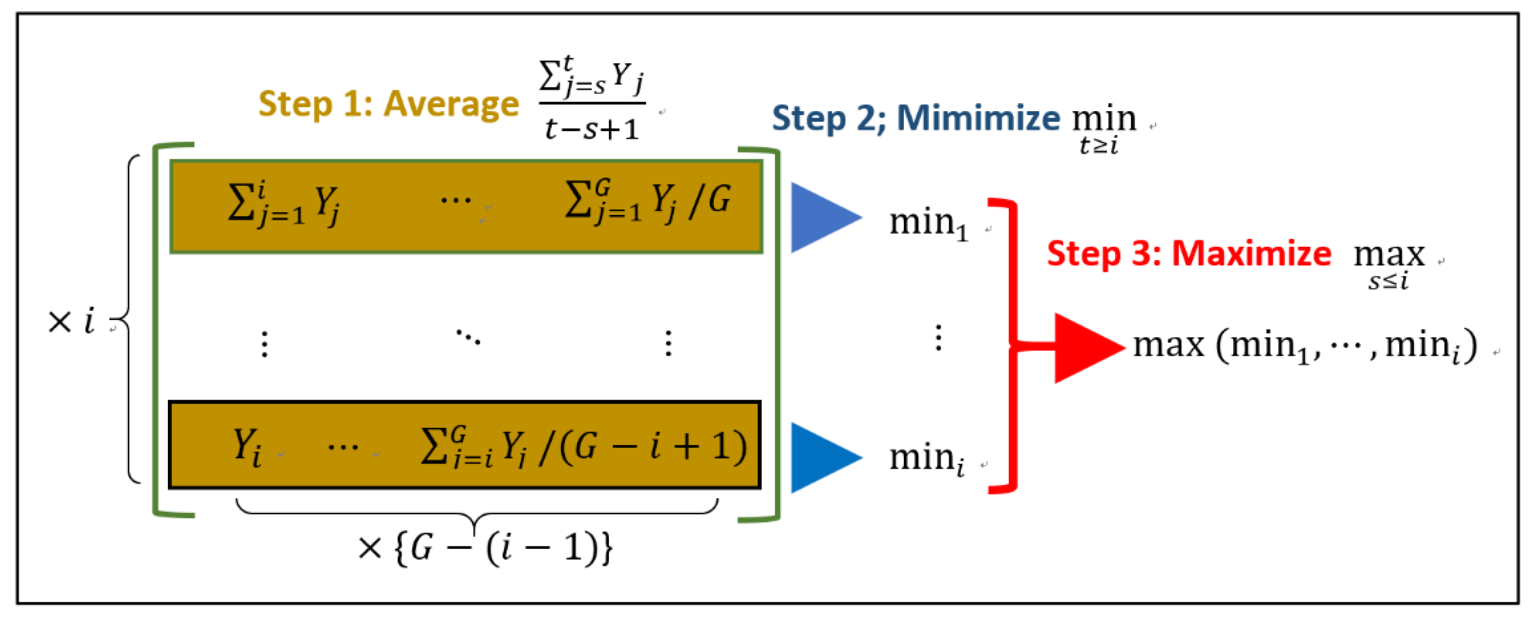
3.2. Restricted Maximum Likelihood Estimators under Ordered Means
3.3. Shrinkage Estimators under Ordered Means
3.4. Estimators under Sparse Means
- alpha1: significance level for (0 < alpha1 < 1);
- alpha2: significance level for (0 < alpha2 < 1);
- q: degrees of shrinkage for (0 < q < 1).
4. Simulation: Validating the R Package
4.1. Simulation Design
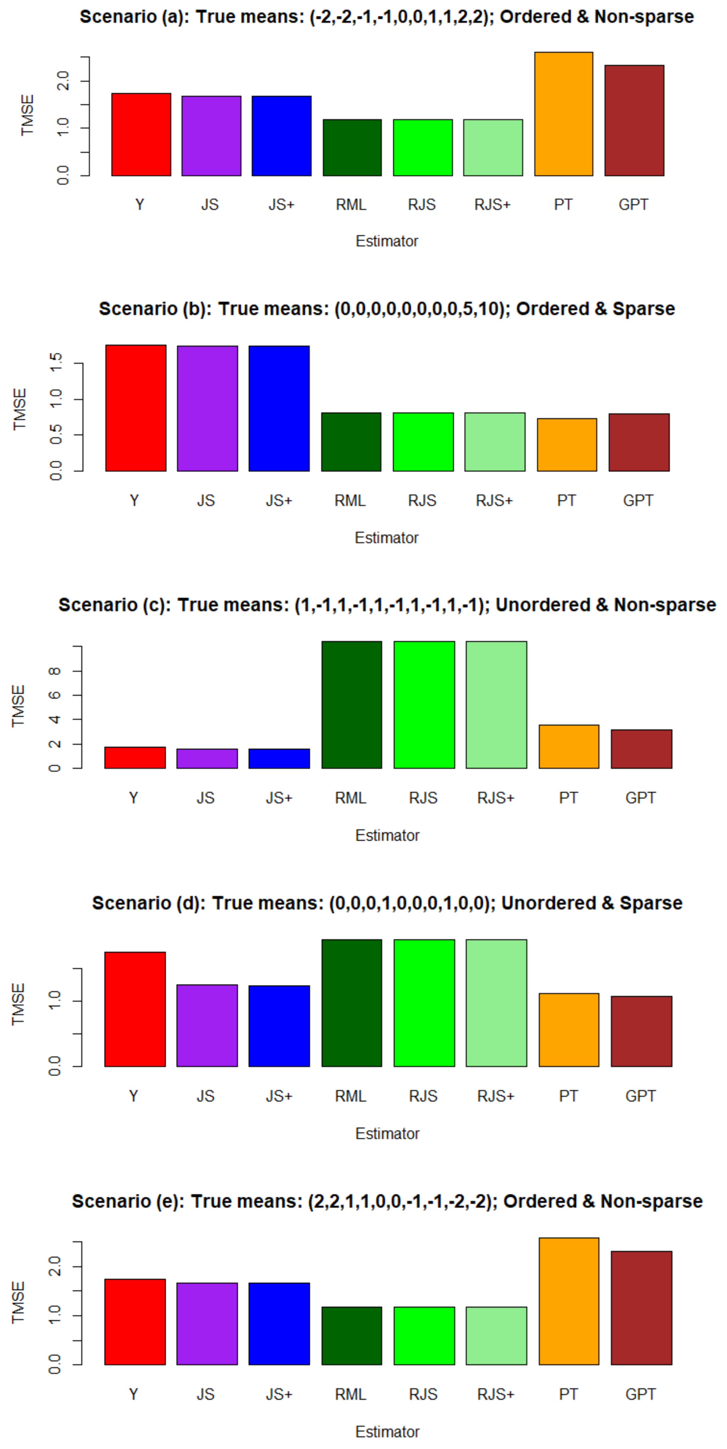
- Scenario (a):
- Ordered and non-sparse: ;
- Scenario (b):
- Ordered and sparse: ;
- Scenario (c):
- Unordered and non-sparse: ;
- Scenario (d):
- Unordered and sparse: ;
- Scenario (e):
- Ordered and non-sparse: ;
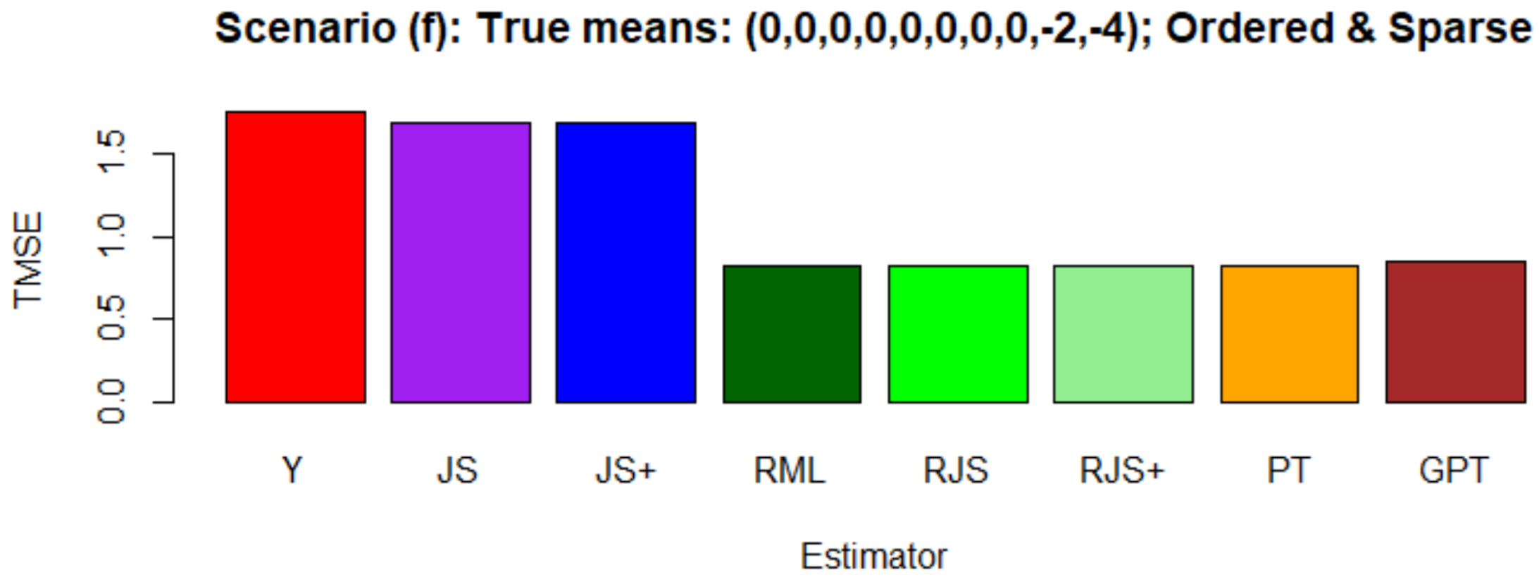
- Scenario (f):
- Ordered and sparse: .
4.2. Simulation Results
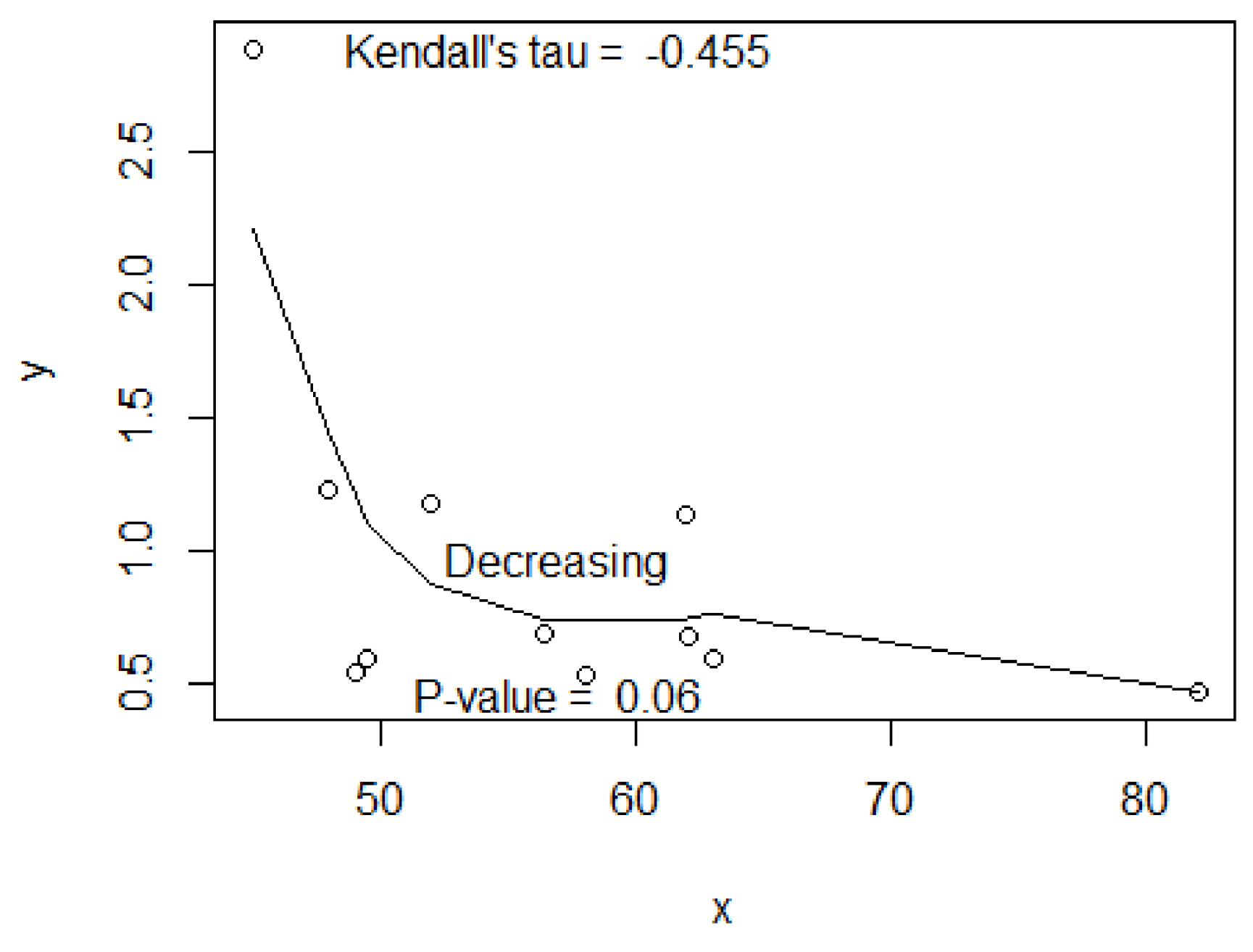
5. Data Example
6. Conclusions and Future Extensions
Supplementary Materials
Author Contributions
Funding
Institutional Review Board Statement
Informed Consent Statement
Data Availability Statement
Acknowledgments
Conflicts of Interest
Appendix A. R Code for Simulations
Appendix B. R Code for the Data Example
References
- Borenstein, M.; Hedges, L.V.; Higgins, J.P.; Rothstein, H.R. Introduction to Meta-Analysis; John Wiley & Sons: Hoboken, NJ, USA, 2011. [Google Scholar]
- Kaiser, T.; Menkhoff, L. Financial education in schools: A meta-analysis of experimental studies. Econ. Educ. Rev. 2020, 78, 101930. [Google Scholar] [CrossRef] [Green Version]
- Leung, Y.; Oates, J.; Chan, S.P. Voice, articulation, and prosody contribute to listener perceptions of speaker gender: A systematic review and meta-analysis. J. Speech Lang. Hear. Res. 2018, 61, 266–297. [Google Scholar] [CrossRef] [PubMed]
- DerSimonian, R.; Laird, N. Meta-analysis in clinical trials revisited. Contemp. Clin. Trials 2015, 45, 139–145. [Google Scholar] [CrossRef] [PubMed] [Green Version]
- Fleiss, J.L. Review papers: The statistical basis of meta-analysis. Stat. Methods Med. Res. 1993, 2, 121–145. [Google Scholar] [CrossRef]
- Batra, K.; Singh, T.P.; Sharma, M.; Batra, R.; Schvaneveldt, N. Investigating the psychological impact of COVID-19 among healthcare workers: A meta-analysis. Int. J. Environ. Res. Public Health 2020, 17, 9096. [Google Scholar] [CrossRef]
- Pranata, R.; Lim, M.A.; Huang, I.; Raharjo, S.B.; Lukito, A.A. Hypertension is associated with increased mortality and severity of disease in COVID-19 pneumonia: A systematic review, meta-analysis and meta-regression. J. Renin-Angiotensin-Aldosterone Syst. 2020, 21, 1470320320926899. [Google Scholar] [CrossRef]
- Wang, Y.; Kala, M.P.; Jafar, T.H. Factors associated with psychological distress during the coronavirus disease 2019 (COVID-19) pandemic on the predominantly general population: A systematic review and meta-analysis. PLoS ONE 2020, 15, e0244630. [Google Scholar] [CrossRef]
- Rice, K.; Higgins, J.P.; Lumley, T. A re-evaluation of fixed effect(s) meta-analysis. J. R. Stat. Soc. Ser. A 2018, 181, 205–227. [Google Scholar] [CrossRef]
- Lehmann, E.L. Elements of Large-Sample Theory; Springer Science & Business Media: Berlin, Germany, 2010. [Google Scholar]
- Shinozaki, N.; Chang, Y.-T. Minimaxity of empirical Bayes estimators of the means of independent normal variables with unequal variances. Commun. Stat.-Theor. Methods 1993, 8, 2147–2169. [Google Scholar] [CrossRef]
- Shinozaki, N.; Chang, Y.-T. Minimaxity of empirical Bayes estimators shrinking toward the grand mean when variances are unequal. Commun. Stat.-Theor. Methods 1996, 25, 183–199. [Google Scholar] [CrossRef]
- Singh, H.P.; Vishwakarma, G.K. A family of estimators of population mean using auxiliary information in stratified sampling. Commun. Stat.-Theor. Methods 2008, 37, 1038–1050. [Google Scholar] [CrossRef]
- DerSimonian, R.; Laird, N. Meta-analysis in clinical trials. Control. Clin. Trials 1986, 7, 177–188. [Google Scholar] [CrossRef]
- Röver, C. Bayesian random-effects meta-analysis using the bayesmeta R package. J. Stat. Softw. 2020, 93, 1–51. [Google Scholar] [CrossRef]
- Raudenbush, S.W.; Bryk, A.S. Empirical bayes meta-analysis. J. Educ. Stat. 1985, 10, 75–98. [Google Scholar] [CrossRef]
- Schmid, C. Using bayesian inference to perform meta-analysis. Eval. Health Prof. 2001, 24, 165–189. [Google Scholar] [CrossRef] [PubMed]
- Röver, C.; Friede, T. Dynamically borrowing strength from another study through shrinkage estimation. Stat. Methods Med. Res. 2020, 29, 293–308. [Google Scholar] [CrossRef] [Green Version]
- Röver, C.; Friede, T. Bounds for the weight of external data in shrinkage estimation. Biom. J. 2021, 63, 1131–1143. [Google Scholar] [CrossRef]
- Taketomi, N.; Konno, Y.; Chang, Y.-T.; Emura, T. A Meta-Analysis for Simultaneously Estimating Individual Means with Shrinkage, Isotonic Regression and Pretests. Axioms 2021, 10, 267. [Google Scholar] [CrossRef]
- Shinozaki, N. A note on estimating the common mean of k normal distributions and the stein problem. Commun. Stat.-Theory Methods 1978, 7, 1421–1432. [Google Scholar] [CrossRef]
- Malekzadeh, A.; Kharrati-Kopaei, M. Inferences on the common mean of several normal populations under hetero-scedasticity. Comput. Stat. 2018, 33, 1367–1384. [Google Scholar] [CrossRef]
- Everitt, B. Modern Medical Statistics: A Practical Guide; Wiley: Hoboken, NJ, USA, 2003. [Google Scholar]
- Lin, L. Hybrid test for publication bias in meta-analysis. Stat. Methods Med. Res. 2020, 29, 2881–2899. [Google Scholar] [CrossRef]
- Lehmann, E.L.; Casella, G. Theory of Point Estimation, 2nd ed.; Springer: New York, NY, USA, 1998. [Google Scholar]
- Shao, J. Mathematical Statistics; Springer: New York, NY, USA, 2003. [Google Scholar]
- van der Pas, S.; Salomond, J.-B.; Schmidt-Hieber, J. Conditions for posterior contraction in the sparse normal means problem. Electron. J. Stat. 2016, 10, 976–1000. [Google Scholar] [CrossRef]
- GASTRIC (Global Advanced/Adjuvant Stomach Tumor Research International Collaboration) Group. Role of chemotherapy for advanced/recurrent gastric cancer: An individual-patient-data meta-analysis. Eur. J. Cancer 2013, 49, 1565–1577. [Google Scholar] [CrossRef] [PubMed]
- James, W.; Stein, C. Estimation with quadratic loss. In Breakthroughs in Statistics; Springer: New York, NY, USA, 1992; Volume 1, pp. 443–460. [Google Scholar]
- van Eeden, C. Restricted Parameter Space Estimation Problems; Springer: New York, NY, USA, 2006. [Google Scholar]
- Li, W.; Li, R.; Feng, Z.; Ning, J. Semiparametric isotonic regression analysis for risk assessment under nested case-control and case-cohort designs. Stat. Methods Med. Res. 2020, 29, 2328–2343. [Google Scholar] [CrossRef] [PubMed]
- Robertson, T.; Wright, F.T.; Dykstra, R. Order Restricted Statistical Inference; Wiley: Chichester, UK, 1988. [Google Scholar]
- Turner, R. Pava: Linear order isotonic regression, Cran. 2020. Available online: https://CRAN.R-project.org/package=Iso (accessed on 14 November 2021).
- Tsukuma, H. Simultaneous estimation of restricted location parameters based on permutation and sign-change. Stat. Pap. 2012, 53, 915–934. [Google Scholar] [CrossRef]
- Chang, Y.-T. Stein-Type Estimators for Parameters Restricted by Linear Inequalities; Faculty of Science and Technology, Keio University: Tokyo, Japan, 1981; Volume 34, pp. 83–95. [Google Scholar]
- Bancroft, T.A. On biases in estimation due to the use of preliminary tests of significance. Ann. Math. Stat. 1944, 15, 190–204. [Google Scholar] [CrossRef]
- Judge, G.G.; Bock, M.E. The Statistical Implications of Pre-Test and Stein-Rule Estimators in Econometrics; Elsevier: Amsterdam, The Netherlands, 1978. [Google Scholar]
- Khan, S.; Saleh, A.K.M.E. On the comparison of the pre-test and shrinkage estimators for the univariate normal mean. Stat. Pap. 2001, 42, 451–473. [Google Scholar] [CrossRef] [Green Version]
- Magnus, J.R. The traditional pretest estimator. Theory Probab. Its Appl. 2000, 44, 293–308. [Google Scholar] [CrossRef]
- Magnus, J.R.; Wan, A.T.; Zhang, X. Weighted average least squares estimation with nonspherical disturbances and an application to the Hong Kong housing market. Comput. Stat. Data Anal. 2011, 55, 1331–1341. [Google Scholar] [CrossRef]
- Shih, J.-H.; Konno, Y.; Chang, Y.-T.; Emura, T. A class of general pretest estimators for the univariate normal mean. Commun. Stat.-Theory Methods 2021. [Google Scholar] [CrossRef]
- Shih, J.-H.; Lin, T.-Y.; Jimichi, M.; Emura, T. Robust ridge M-estimators with pretest and Stein-rule shrinkage for an intercept term. Jpn. J. Stat. Data Sci. 2021, 4, 107–150. [Google Scholar] [CrossRef]
- Kibria, B.G.; Saleh, A.M.E. Optimum critical value for pre-test estimator. Commun. Stat.-Simul. Comput. 2006, 35, 309–319. [Google Scholar] [CrossRef]
- Shih, J.-H.; Konno, Y.; Chang, Y.-T.; Emura, T. Estimation of a common mean vector in bivariate meta-analysis under the FGM copula. Statistics 2019, 53, 673–695. [Google Scholar] [CrossRef]
- Gleser, L.J.; Olkin, L. Stochastically dependent effect sizes. In the Handbook of Research Synthesis; Russel Sage Foundation: New York, NY, USA, 1994. [Google Scholar]
- Shih, J.-H.; Konno, Y.; Chang, Y.-T.; Emura, T. Copula-based estimation methods for a common mean vector for bivariate meta-analyses. Symmetry 2021, in press. [Google Scholar]
- Emura, T.; Sofeu, C.L.; Rondeau, V. Conditional copula models for correlated survival endpoints: Individual patient data meta-analysis of randomized controlled trials. Stat. Methods Med. Res. 2021, 30, 2634–2650. [Google Scholar] [CrossRef] [PubMed]
- Mavridis, D.; Salanti, G.A. practical introduction to multivariate meta-analysis. Stat. Methods Med. Res. 2013, 22, 133–158. [Google Scholar] [CrossRef] [PubMed]
- Peng, M.; Xiang, L.; Wang, S. Semiparametric regression analysis of clustered survival data with semi-competing risks. Comput. Stat. Data Anal. 2018, 124, 53–70. [Google Scholar] [CrossRef]
- Peng, M.; Xiang, L. Correlation-based joint feature screening for semi-competing risks outcomes with application to breast cancer data. Stat. Methods Med. Res. 2021, 30, 2428–2446. [Google Scholar] [CrossRef]
- Riley, R.D. Multivariate meta-analysis: The effect of ignoring within-study correlation. J. R. Stat. Soc. Ser. A 2009, 172, 789–811. [Google Scholar] [CrossRef]
- Copas, J.B.; Jackson, D.; White, I.R.; Riley, R.D. The role of secondary outcomes in multivariate meta-analysis. J. R. Stat. Soc. Ser. C 2018, 67, 1177–1205. [Google Scholar] [CrossRef]
- Sofeu, C.L.; Emura, T.; Rondeau, V. A joint frailty-copula model for meta-analytic validation of failure time surrogate endpoints in clinical trials. BioMed. J. 2021, 63, 423–446. [Google Scholar] [CrossRef] [PubMed]
- Yamaguchi, Y.; Maruo, K. Bivariate beta-binomial model using Gaussian copula for bivariate meta-analysis of two binary outcomes with low incidence. Jpn. J. Stat. Data Sci. 2019, 2, 347–373. [Google Scholar] [CrossRef] [Green Version]
- Kawakami, R.; Michimae, H.; Lin, Y.-H. Assessing the numerical integration of dynamic prediction formulas using the exact expressions under the joint frailty-copula model. Jpn. J. Stat. Data Sci. 2021, 4, 1293–1321. [Google Scholar] [CrossRef]
- Nikoloulopoulos, A.K. A vine copula mixed effect model for trivariate meta-analysis of diagnostic test accuracy studies accounting for disease prevalence. Stat. Methods Med. Res. 2017, 26, 2270–2286. [Google Scholar] [CrossRef] [PubMed] [Green Version]
- Karamikabir, H.; Afshari, M. Generalized Bayesian shrinkage and wavelet estimation of location parameter for spherical distribution under balance-type loss: Minimaxity and admissibility. J. Multivar. Anal. 2020, 177, 104583. [Google Scholar] [CrossRef]
- Bilodeau, M.; Kariya, T. Minimax estimators in the normal MANOVA model. J. Multivar. Anal. 1989, 28, 260–270. [Google Scholar] [CrossRef] [Green Version]
- Konno, Y. On estimation of a matrix of normal means with unknown covariance matrix. J. Multivar. Anal. 1991, 36, 44–55. [Google Scholar] [CrossRef] [Green Version]
- Karamikabir, H.; Afshari, M.; Lak, F. Wavelet threshold based on Stein’s unbiased risk estimators of restricted location parameter in multivariate normal. J. Appl. Stat. 2021, 48, 1712–1729. [Google Scholar] [CrossRef]
- Pandey, B.N. Testimator of the scale parameter of the exponential distribution using LINEX loss function. Commun. Stat.-Theory Methods 1997, 26, 2191–2202. [Google Scholar] [CrossRef]
- Vishwakarma, G.K.; Gupta, S. Shrinkage estimator for scale parameter of gamma distribution. Commun. Stat.-Simul. Comput. 2020. [Google Scholar] [CrossRef]
- Chang, Y.-T.; Shinozaki, N. New types of shrinkage estimators of Poisson means under the normalized squared error loss. Commun. Stat.-Theory Methods 2019, 48, 1108–1122. [Google Scholar] [CrossRef]
- Hamura, Y. Bayesian shrinkage approaches to unbalanced problems of estimation and prediction on the basis of negative multinomial samples. Jpn. J. Stat. Data Sci. 2021. [Google Scholar] [CrossRef]
- Soliman, A.-A.; Abd Ellah, A.H.; Sultan, K.S. Comparison of estimates using record statistics from Weibull model: Bayesian and non-Bayesian approaches. Comput. Stat. Data Anal. 2006, 51, 2065–2077. [Google Scholar] [CrossRef]
- Rehman, H.; Chandra, N. Inferences on cumulative incidence function for middle censored survival data with Weibull regression. Jpn. J. Stat. Data Sci. 2022. [Google Scholar] [CrossRef]


| Treatment Effect on SBP | SE | Treatment Effect on DBP | SE | |
|---|---|---|---|---|
| Study 1 | −6.66 | 0.72 | −2.99 | 0.27 |
| Study 2 | −14.17 | 4.73 | −7.87 | 1.44 |
| Study 3 | −12.88 | 10.31 | −6.01 | 1.77 |
| Study 4 | −8.71 | 0.30 | −5.11 | 0.10 |
| Study 5 | −8.70 | 0.14 | −4.64 | 0.05 |
| Study 6 | −10.60 | 0.58 | −5.56 | 0.18 |
| Study 7 | −11.36 | 0.30 | −3.98 | 0.27 |
| Study 8 | −17.93 | 5.82 | −6.54 | 1.31 |
| Study 9 | −6.55 | 0.41 | −2.08 | 0.11 |
| Study 10 | −10.26 | 0.20 | −3.49 | 0.04 |
| Covariate | |||||||
|---|---|---|---|---|---|---|---|
| Study 2 | −7.87 | −17.93 | −17.91 | −17.91 | −16.05 | −16.05 | −16.05 |
| Study 8 | −6.54 | −10.26 | −10.25 | −10.25 | −16.05 | −16.05 | −16.05 |
| Study 3 | −6.01 | −14.17 | −14.16 | −14.16 | −12.88 | −12.88 | −12.88 |
| Study 6 | −5.56 | −11.36 | −11.35 | −11.35 | −10.6 | −10.6 | −10.6 |
| Study 4 | −5.11 | −8.71 | −8.70 | −8.70 | −9.76 | −9.76 | −9.76 |
| Study 5 | −4.64 | −10.6 | −10.59 | −10.59 | −9.76 | −9.76 | −9.76 |
| Study 7 | −3.98 | −8.7 | −8.69 | −8.69 | −9.76 | −9.76 | −9.76 |
| Study 10 | −3.49 | −12.88 | −12.87 | −12.87 | −9.76 | −9.76 | −9.76 |
| Study 1 | −2.99 | −6.66 | −6.65 | −6.65 | −6.66 | −6.66 | −6.66 |
| Study 9 | −2.08 | −6.55 | −6.54 | −6.54 | −6.55 | −6.55 | −6.55 |
Publisher’s Note: MDPI stays neutral with regard to jurisdictional claims in published maps and institutional affiliations. |
© 2022 by the authors. Licensee MDPI, Basel, Switzerland. This article is an open access article distributed under the terms and conditions of the Creative Commons Attribution (CC BY) license (https://creativecommons.org/licenses/by/4.0/).
Share and Cite
Taketomi, N.; Michimae, H.; Chang, Y.-T.; Emura, T. meta.shrinkage: An R Package for Meta-Analyses for Simultaneously Estimating Individual Means. Algorithms 2022, 15, 26. https://doi.org/10.3390/a15010026
Taketomi N, Michimae H, Chang Y-T, Emura T. meta.shrinkage: An R Package for Meta-Analyses for Simultaneously Estimating Individual Means. Algorithms. 2022; 15(1):26. https://doi.org/10.3390/a15010026
Chicago/Turabian StyleTaketomi, Nanami, Hirofumi Michimae, Yuan-Tsung Chang, and Takeshi Emura. 2022. "meta.shrinkage: An R Package for Meta-Analyses for Simultaneously Estimating Individual Means" Algorithms 15, no. 1: 26. https://doi.org/10.3390/a15010026
APA StyleTaketomi, N., Michimae, H., Chang, Y.-T., & Emura, T. (2022). meta.shrinkage: An R Package for Meta-Analyses for Simultaneously Estimating Individual Means. Algorithms, 15(1), 26. https://doi.org/10.3390/a15010026