An Effective Atrial Fibrillation Detection from Short Single-Lead Electrocardiogram Recordings Using MCNN-BLSTM Network

Abstract

Atrial fibrillation (AF) is an arrhythmia that may cause blood clots and increase the risk of stroke and heart failure. Traditional 12-lead electrocardiogram (ECG) acquisition equipment is complex and difficult to carry. Short single-lead ECG recordings based on wearable devices can remedy these shortcomings. However, reliable and accurate atrial fibrillation detection is still an issue because of the limited information on the short single-lead ECG recordings. In this paper, we propose a novel multi-branch convolutional neural network and bidirectional long short-term memory network (MCNN-BLSTM) to deal with the reliability and accuracy of AF detection in short single-lead ECG recordings. Firstly, to fuller extract the feature information of short single-lead ECG recordings, the MCNN module is designed to dynamically set several corresponding branches according to the number of slices of short single-lead ECG recordings. Then, the BLSTM module is designed to further enhance the feature information learned from each branch. We validated the model on the PhysioNet/CinC Challenge 2017 (CinC2017) database and verified the generalization of the model on the China Physiological Signal Challenge 2018 (CPSC2018) database. The results show that the accuracy of the model on the CinC 2017 database reaches 87.57%, and the average F1 score reaches 84.56%. The accuracy of the model on the CPSC 2018 database reaches 87.50%, and the average F1 score reaches 82.01%. Compared with other advanced methods, our model shows better performance and can meet the daily needs of atrial fibrillation detection with short ECG wearable devices.

1. Introduction

Atrial fibrillation (AF) is a common supraventricular arrhythmia. According to statistics, the number of AF patients in adults is about 2% to 4%, and the number is increasing [1]. Although AF does not directly lead to death, it significantly impacts people’s health. This arrhythmia can lead to high morbidity and mortality, resulting in a considerable investment of health resources, which can impose a significant economic burden on society. The presentation of AF is usually asymptomatic and may not be detected until a thromboembolic event occurs. The prevalence of AF increases with age. The dynamic electrocardiogram (ECG) is one of the essential tools for detecting AF [1,2,3]. However, wearing a traditional ECG monitor is not only inconvenient, but also interferes with a lot of daily life. In recent years, wearable devices have become increasingly popular for AF detection. Therefore, using different measurement techniques to detect AF using short single-lead ECG recordings is very important [4].

Wearable devices provide a cheaper and more convenient solution for AF detection [5]. For short single-lead ECG recordings, signal processing methods are particularly important due to different signal lengths. Warrick et al. [6] used the clipping and filling method to process ECG recordings of various sizes into fixed-length sequences. However, this method may lead to the loss of information in the input samples to the extent that the samples cannot be fully utilized. Lee et al. [7] applied the consistent-sized electrocardiomatrix (CS-ECM) method to processing short-term ECG signals, avoiding the segmentation of short single-lead ECG recordings. However, such a method had information redundancy for short single-lead ECG recordings, and the redundant information did not provide more feature information for the model. Fang et al. [8] extracted the time-frequency spectrum and Poincare plot of ECG signals, respectively. It avoided the segmentation processing of short single-lead ECG recordings. However, such a signal pretreatment operation was too complicated, reducing the model’s real-time performance. Although there are many processing methods for short single-lead ECG recordings, choosing an appropriate method that can fully use the limited dynamic ECG information is still a problem.

The main features of the AF signal are the irregular R-R intervals (when atrioventricular conduction is not impaired), the absence of distinct repeating P waves, and irregular atrial activations [1,9]. In the early studies, most of the machine learning (ML) methods were used to achieve AF detection. Tang et al. [10] proposed a hybrid Taguchi-genetic algorithm to decompose ECG signals and obtain p-wave amplitude features for AF detection. Compared with p-wave features, the QRS complex has a higher amplitude and is easier to locate. Therefore, the method based on RR interval features is widely used in AF detection. Sadr et al. [11] used the time domain, frequency domain, and distribution feature of RR interval to achieve AF classification of short single-lead ECG recordings. Zhao et al. [12] detected RR features of AF by measuring signal entropy. However, the method based on RR interval features mainly relies on the local localization of the QRS complex to extract the RR interval, and the classification models primarily relied on the QRS complex localization algorithm. Hence, the two parts produce a great degree of coupling. In addition, ML methods are mainly based on manual feature extraction and feature selection, requiring multiple steps to complete the final classification [13], and the process is relatively complex.

Deep learning (DL) has the ability of feature learning and classification [14], so various DL methods have been widely applied in AF detection, including convolutional neural networks (CNN) [7,8,15,16,17] and recurrent neural networks (RNN) [18]. Lee et al. [7] proposed a beat-interval-texture convolutional neural network (BIT-CNN) model based on CNN to extract AF signal features and achieve AF detection through simultaneous one-dimension and two-dimensional convolution of two-dimensional image CS-ECM. Zhang et al. [19] proposed a specific-scale stationary wavelet transform processing method to analyze the time-frequency features of ECG signals and used the scale-independent convolutional neural network to extract the time-domain and frequent-domain features of ECG signals, and finally realized better AF detection on the MIT-BIH Atrial Fibrillation database. Kamaleswaran et al. [17] proposed a 13-layer deep CNN network model for detecting AF in short single-lead ECG recordings. Fan et al. [20] designed a multi-scale fusion convolutional neural network to solve the problem of AF detection of short single-lead ECG recordings. In this case, two CNNs with different sizes of convolution kernels were set up to extract ECG recordings features of different scales. Cao et al. [18] proposed a data enhancement strategy based on ECG, and on this basis, realized the automatic detection of AF using the double-layer LSTM model. Mehrang et al. [21] obtained seismocardiography and gyrocardiography signals separately by smartphone, and used BLSTM to learn the time series features of the signal, and squeeze-and-excitation (SE) blocks learned the interdependence between channels. Andersen et al. [22] proposed a network model that combined CNN and LSTM. The model realized AF detection by directly extracting the RR interval sequence of the ECG signal as input, and verified it on multiple databases. The results showed that the model also had a stable performance on other databases. Fang et al. [8] proposed a dual-channel neural network based on the visual geometry group (VGG) network, in which features were extracted from the time spectrum and Poincare diagram of ECG signals simultaneously, thus achieving effective detection of AF. Lu et al. [23] proposed a multichannel parallel neural network model (MLCNN-BiLSTM). MLCNN was used for feature extraction in the model with multi-lead ECG signals, and BiLSTM was used for timing feature extraction in the second lead. Finally, the two features were weighted and integrated to classify arrhythmias better. Today, the output of deep learning models is comparable with human experts and sometimes achieves even better results [24].

Although ML and DL have achieved good results in detecting atrial fibrillation, the critical problem of real-time atrial fibrillation detection is still not solved. Since most AF detection methods are based on static ECG signals, the applicability of the dynamic ECG signal is limited. In particular, in limited short single-lead ECG recordings, reliable and accurate AF detection remains challenging. To solve the above problems and improve the ability of short single-lead ECG recordings in atrial fibrillation detection, we propose a novel short single-lead ECG recordings AF detection model (MCNN-BLSTM), which is mainly composed of the MCNN module and BLSTM module. First, the MCNN module can set the corresponding branch according to the number of fragments obtained by the overlapping segmentation scheme for feature extraction. Such a feature extraction method can retain the sensing ability of local features of the model and keep the dependence between heartbeats to a certain extent. Then, the BLSTM module is used to strengthen the feature information extracted from each branch to improve the detection ability of the model. Finally, the ablation experiment verifies the effectiveness of our model. We evaluate the performance of the MCNN-BLSTM model on two databases (the CinC2017 database and the CPSC2018 database) and verify the reliability of the proposed model by visual analysis of the features learned from the model.

The rest of the paper is organized as described in the following: Section 2 introduces the databases used in this paper and the model framework of MCNN-BLSTM. Section 3 presents the detailed experimental process. Section 4 discusses the model proposed in this paper. Finally, Section 5 summarizes the work of this paper and suggests the future research direction.

2. Materials and Methods

2.1. Materials

Two open databases are used in this study, PhysioNet/CinC Challenge 2017 (CinC2017) [25] and China Physiological Signal Challenge 2018 (CPSC2018) [26].

1.

CinC2017: The CinC2017 ECG recordings were collected using the AliveCor facility. The officially published training set contains 8528 single-lead recordings. These recordings have different lengths, ranging from 9 s to 61 s. The sampling rate is 300 Hz. This database contains a total of four rhythm types, namely, normal rhythm (N), atrial fibrillation rhythm (A), other rhythms (O), and noise. The detailed content of the database is shown in

Table 1. Databases description.

Database	Rhythm	#Number of Recordings	Time Length(s)
			Mean	Min	Max
PhysioNet/CinC Challenge 2017	Normal	5050	32.10	9.05	60.95
	AF	738	32.10	9.99	60.21
	Other	2456	34.39	9.13	60.86
	Noise	284	24.22	9.36	60.00
China Physiological Signal Challenge 2018	Normal	918	15.43	10.00	60.00
	AF	1098	15.04	9.00	74.00
	Other	4861	16.25	6.00	144.00

.

2.

CPSC2018: The CPSC2018 database includes 6877 recordings collected from the officially issued training set of 11 hospitals, and each sample contains standard 12-lead signals. Here, we use the second lead for testing. The recordings varied in length, ranging from 6 s to 144 s. The sampling rate is 500 Hz. The database contained a total of nine rhythmic types. We organized the data from the CPSC2018 database into three categories: N, AF, and O. Our goal is to screen AF patients based on their short ECG recordings, and the database is detailed in Table 1.

2.2. Methods

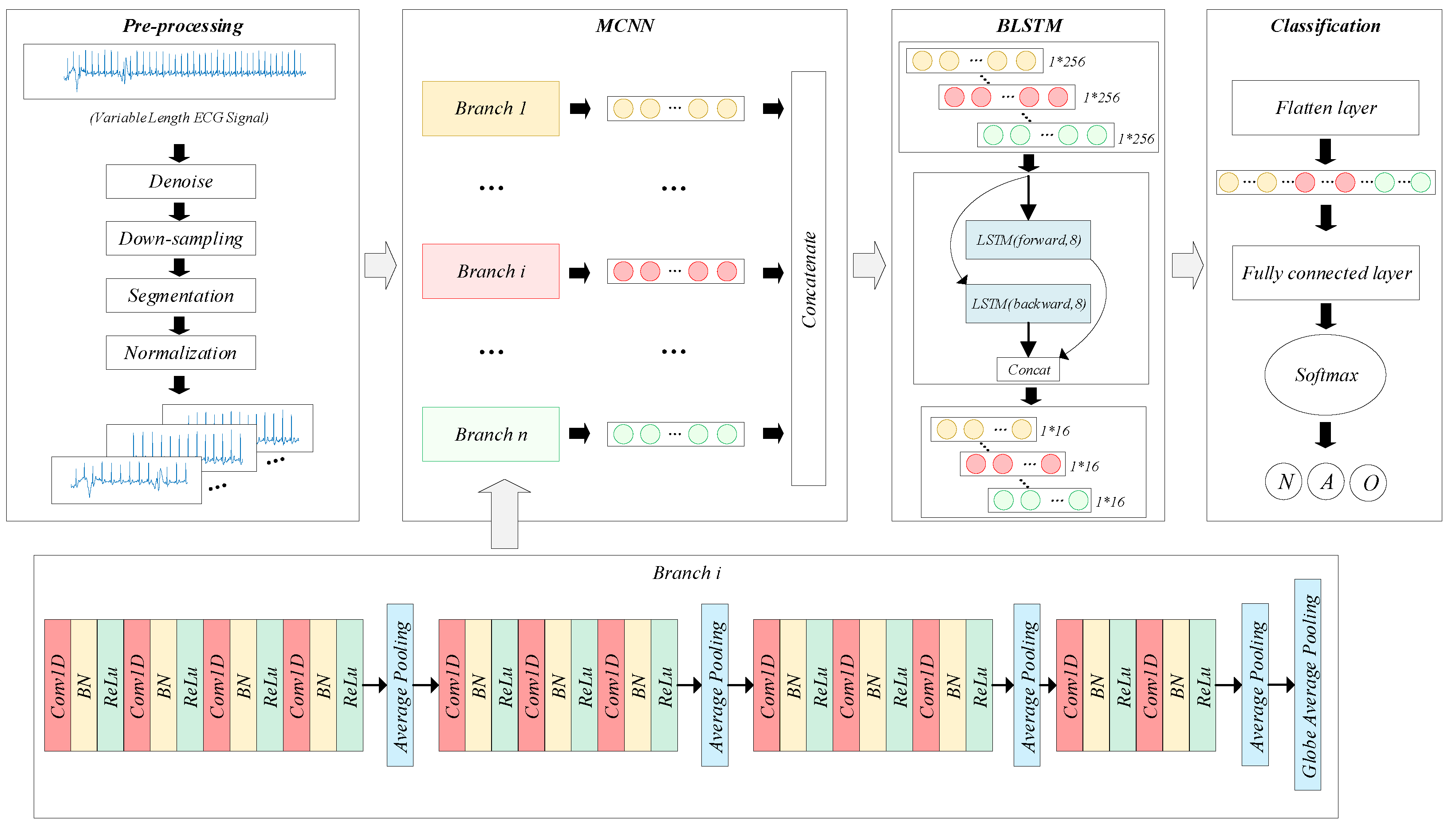
2.2.1. Pre-Processing

In this study, the Daubechies 6 wavelet transform [27] performs a nine-level wavelet decomposition on the original ECG signal, eliminates the D1, D2, and A9 components, and reconstructs the remaining components to obtain the filtered signal. We used the down-sampling strategy [20] to down-sample all the ECG signals in the two databases to 120 Hz. Down-sampling is the process of reducing the sampling rate of ECG recordings, which helps to reduce the complexity of the model.

The short-term ECG recordings used in this study had unequal signal lengths. In the CinC2017 database, the shortest recording was 9 s, and the longest was 61 s. In the CSPC2018, the shortest recording was 6 s, and the longest was 144 s. Thus, we use a scheme of overlapping slices [28]. The length of the overlap is calculated as follows:

$$ol=⌊l-(L-l)/(n-1)⌋$$

(1)

where L is the length of an ECG recording, n is the number of segments, l is the length of each segment, and $ol$ is the length of the overlap between two adjacent segments.

Different people demonstrate different amplitudes of ECG recordings. Even for the same individual, the amplitude of ECG recording varies. Standardizing the input data can prevent the MCNN-BLSTM model from experiencing a gradient explosion during training, and it can make the model converge faster. In this study, the z-score normalization technology is used to make the magnitude of the ECG signal subject to uniform data distribution. Z-score can be defined as follows:

$$x^{*}=\frac{x-E\left(x\right)}{\sqrt{Var\left(x\right)}}$$

(2)

where $E\left(x\right)$ is the mean of the ECG samples, and $Var\left(x\right)$ is the variance of the ECG samples.

Finally, we split 20% of the processed database into the testing set, 10% of the remaining data into the validation set, and the rest into the training set.

2.2.2. Problem Description

In the experiment of this paper, let $D=\left\{\left(x^{\left(1\right)},y^{\left(1\right)}\right),\cdots ,\left(x^{\left(i\right)},y^{\left(i\right)}\right),\cdots ,\left(x^{\left(m\right)},y^{\left(\mathrm{m}\right)}\right)\right\}$ be the training set, m is the number of ECG recordings, $x^{\left(i\right)}$ is the ith ECG recording (Note that the lengths of the input ECG recordings are not equal), $y^{\left(i\right)}\in \left\{0,1,2\right\}$ is the class label of the ith ECG recording, 0 represents a normal rhythm, 1 represents an AF rhythm, and 2 represents the other rhythm. The model output is $z^{\left(i\right)}$ for an ECG recording $x^{\left(i\right)}$. The formula is shown as follows:

$$\begin{array}{c}\hfill z^{\left(i\right)}=g\left(x^{\left(i\right)};\theta \right)\end{array}$$

(3)

where $\theta$ is the relevant parameter in the proposed model.

After calculating the feature vector $z^{\left(i\right)}$ of each class, $z^{\left(i\right)}$ is fed to a linear layer whose output length is the number of categories, and the softmax function is added to output the probability that the ECG recording is a normal rhythm, AF rhythm, or other rhythms. The corresponding softmax function is calculated as follows:

$${\widehat{y}}^{\left(i\right)}=\frac{exp\left(z^{\left(i\right)}\right)}{{\sum }_{j=1}^{c}exp\left(z^{\left(j\right)}\right)}$$

(4)

where c is the number of ECG rhythm classes, and ${\widehat{y}}^{\left(i\right)}$ indicates the class probability of the input feature vector $z^{\left(i\right)}$.

2.2.3. Model Architecture

The proposed MCNN-BLSTM model structure is shown in Figure 1. In this model, an ECG recording is segmented into n ECG segments and input into n branches. Each branch is a 1-dimensional CNN network, which extracts an ECG partial segment feature with a duration of l s. To improve the detection rate of AF, we combine the features extracted by every branch and use them as the input to BLSTM to enhance the temporal features. Finally, the classification is performed using a softmax layer.

1.

MCNN: For the MCNN considered in this study, the number n of branches is set based on the slice length l which is chosen as 6 s, 10 s, 15 s, 20 s, 25 s, and 30 s. Thus, $n=⌈\left(L_{max}\right)/l⌉$, where L is the length of a short ECG recording, and l is the length of each ECG segment. Each short ECG recording has a different length. To make full use of the information from one ECG recording, we adopted the overlapping cutting scheme. The overlapping part is calculated using Equation (1). Thus, the MCNN could extract the entire short ECG recording feature, which improves the inadequacy of the 1-branch CNN (1BCNN) that could not extract all the ECG information.

In MCNN, each branch consists of 12 convolutional layers and four pooling layers, grouped by convolutional layers and separated by a pooling layer. Therefore, each 1BCNN consists of four groups of convolutional layers. The number of convolutional layers in the four convolution groups is 4, 3, 3, and 2. The number of filters in the first group is 8, 16, 32, and 32. There are 64 filters in the second group. The third group has 128 filters. The last group of convolutional layers has 256 filters. Output data are processed using batch normalization (BN) [29] to solve the problem of an internal covariate shift. It has the advantage of allowing the model to use a higher learning rate during the training process, which could reduce the possibility of the over-fitting of the layer.

In addition, the pooling layer of each group uses average pooling (AP), and the last layer uses global average pooling (GAP). The pooling layer has the advantages of data dimensionality reduction, nonlinear transformation, and expansion of the perception field. In each branch, the pooling layer step size is set to four to quickly reduce the computational complexity and capture the local features between the ECG recordings within a short time window. The last group of convolutions is used by the GAP instead of the AP. GAP [30] mainly performs a pooling of the entire feature map of the last layer to form a feature point. It is mainly proposed to solve the problem of full connection, as there are too many parameters in the full connection operation. One advantage of GAP over a fully connected layer is that it has no parameters that need to be optimized. Thus, overfitting of the layer is avoided. Additionally, GAP can extract spatial information and is more robust to the spatial transformation of the inputs. Let $f_k(a,b)$ be the activation value of element k in the last convolutional layer on the feature space location $(a,b)$. For unit k, the result $F_k={\sum }_{a,b}{f}_k(a,b)$ of the GAP was obtained.

2.

LSTM: LSTM is one kind of recurrent neural network. Unlike the traditional RNN, LSTM can effectively deal with the long-term dependence of temporal signals [31]. The computational process of LSTM is more complex than RNN, and the main computational process is shown following:

$$f_t=sigmoid\left(W_f·\left[a_{t-1},x_t,c_{t-1}\right]+b_f\right)$$

(5)

$$i_t=sigmoid\left(W_i·\left[a_{t-1},x_t,c_{t-1}\right]+b_i\right)$$

(6)

$$c_{in}=tanh\left(W_c·\left[a_{t-1},x_t,c_{t-1}\right]+b_c\right)$$

(7)

$$c_t=f_t·c_{t-1}+i_t·c_{in}$$

(8)

$$o_t=sigmoid\left(W_o·\left[a_{t-1},x_t,c_{t-1}\right]+b_o\right)$$

(9)

$$a_t=o_t·tanh\left(c_t\right)$$

(10)

where $f_t$, $i_t$, $o_t$, and $c_t$ are the forget gate, input gate, output gate, and the cell unit information vector, respectively. W denotes a weight matrix (e.g., $W_i$ is the weight matrix of the input gate), and b denotes an offset vector (e.g., $b_i$ is the offset vector of the input gate). When the forget gate $f_t$ or the input gate $i_t$ is activated, the value stored in cell unit $c_t$ is updated. The output gate $o_t$ controls the value in the cell to be output from the LSTM cell.

Compared with LSTM, BLSTM can fetch both the preceding and the following context information, avoiding the disadvantage that LSTM networks can only extract the preceding context information [22]. In this paper, we used BLSTM to consider 256 ECG features of the n segments extracted by the MCNN, the n segments are segmented in the chronological order of the ECG recording. Finally, a $softmax$ layer is used to predict the type of one input ECG recording (normal, AF, or other rhythms).

2.3. Model Training

The current more popular gradient descent algorithms include the following: Adam [32], stochastic gradient descent (SGD), and AdaGrad [33]. To reduce the training time of each time step, the SGD algorithm is introduced earlier. However, the SGD algorithm is subject to local saddle points in some cases due to its drawbacks. Therefore, momentum is introduced to accelerate the convergence of the model in the correct direction and reduce the possibility that the model falls into the local optimum. The AdaGrad algorithm can dynamically adjust the learning rate during training. When the number of parameter updates is long, the learning rate decreases, while when the number of parameter updates is small, the learning rate increases. Adam uses the first-order moment estimation and the second-order moment estimation of the gradient to dynamically adjust the learning rate of each parameter. Each iteration learning rate has a certain range, which makes the parameter update relatively stable. SGD is the most commonly used method to optimize the CNN network [34]. In this study, SGD with a batch size of 32 is used. The initial learning rate is 0.1, and the exponential learning rate decay is 10 times in every 10 epochs, the maximum number of early stop epochs to 100 by default. The learning rate $\eta$ decayed as follows:

$$\eta ={\eta }_0*0.1^{N/\phantom{N10}10}$$

(11)

where ${\eta }_0$ is the initial learning rate, and N is the number of epochs.

Overfitting is a common phenomenon in machine learning. It is manifested as the model is trained with higher accuracy on the training set and lower accuracy on the testing set. The noises and individual differences in the ECG signals are the main factors leading to the overfitting of the model. To prevent overfitting, regularization techniques in the proposed model are used. During the proposed model training process, the L2 regularization parameters of each convolutional layer of the MCNN module were added to the loss function. Therefore, our loss function can be defined as follows:

$$L\left(x\right)=-\frac{1}{\left|D\right|}{\sum }_{i=1}^{\left|D\right|}log{\widehat{y}}^{\left(i\right)}+\lambda {∥W∥}^2$$

(12)

where $\left|D\right|$ is the size of the training set, ${\widehat{y}}^{\left(i\right)}$ is calculated using Equation (4), $\lambda$ is the penalty factor, and W is the weight parameter in the proposed model.

Another regularization method is the dropout technique [35]. The dropout technique effectively alleviates the overfitting of the model by stopping certain neurons during the training process. L2 regularization is achieved by modifying the loss function to reduce overfitting, while dropout is achieved by modifying the network. For the ECG signal recording whose length is less than the average ECG recording length, the information between the segments is redundant. To alleviate this situation, the dropout technology between MCNN and BLSTM is added, and set the p-value to 0.4.

Finally, the default parameter settings of the model are shown in

Table 2. Related parameter settings for the model proposed in this study.

Learning Parameter	Values
Weight penalty	L2-norm
Trade-off parameter	0.001
Optimizer	SGD
Learning rate initial value	0.10
Dropout proportion	0.40
Batch size	32
Momentum coefficient	0.70
Number of epochs	100

, in which all parameters are the optimal values selected after the experiment.

3. Results

This study is based on Ubuntu 64-bit operating system, the CPU is Intel (R) Core i9 processor, the GPU is NVIDIA GeForce RTX2080TI, and the running memory is 64 G. The model framework is based on TensorFlow 2.1.0.

3.1. Evaluation Metrics

For the detection of AF, the classification performance of the MCNN-BLSTM model is evaluated using five criteria: accuracy (ACC), recall (REC), precision (PRE), specificity (SPE), and F1 score. The above-mentioned evaluation criteria could be expressed by a confusion matrix (

Table 3. Confusion matrix.

		Predicted
		Positive	Negative
Reference	Positive	TP	FN
	Negative	FP	TN

). AF is defined as a positive class. Then, the five criteria are defined as follows:

$$ACC=\frac{TPs+TNs}{TPs+TNs+FPs+FNs}$$

(13)

$$REC=\frac{TPs}{TPs+FNs}$$

(14)

$$PRE=\frac{TPs}{TPs+FPs}$$

(15)

$$SPE=\frac{TNs}{TNs+FPs}$$

(16)

$$F1=\frac{2\times REC\times PRE}{REC+PRE}$$

(17)

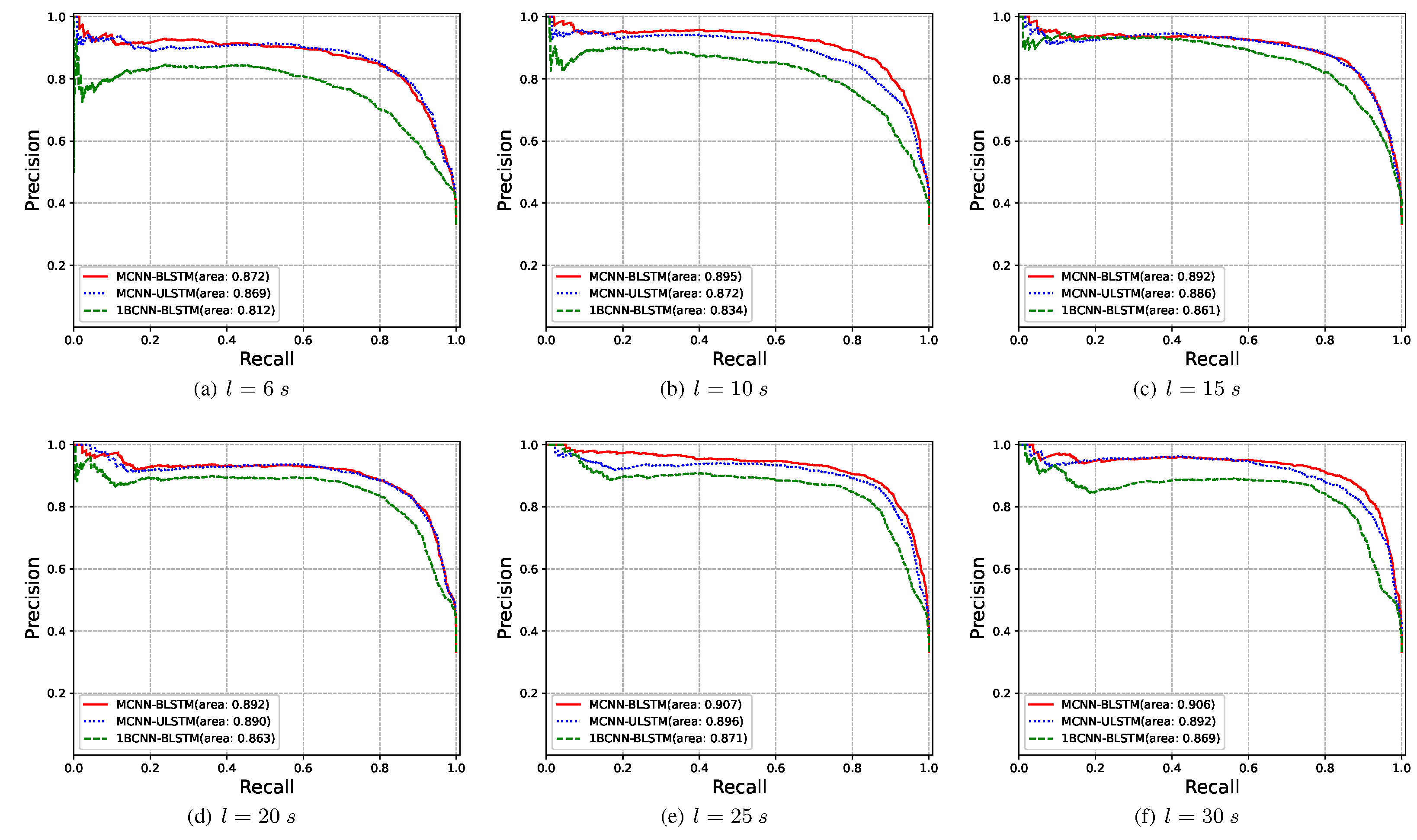
3.2. Ablation Experiments

To prove the effectiveness of the proposed MCNN-BLSTM model, we designed the following two models for ablation experiments:

1.

1BCNN-BLSTM: The model has the same structure as MCNN-BLSTM, but can only input a single branch ECG signal. When the length L of the segment is longer than the original ECG recording, zero padding is performed for the segment length. When the length of the segment is shorter than the original ECG recording, the ECG segment with the front length L of the original ECG recording is intercepted and used as the input of the model.

2.

MCNN-ULSTM: The model has the same structure as MCNN-BLSTM, but BLSTM was modified to ULSTM to verify the influence of the BLSTM module on atrial fibrillation detection.

In this study, we used short single-lead ECG recordings for atrial fibrillation detection. The MCNN module can set branch numbers according to the input ECG recordings and segment length. Here, the segment length l is set to 6 s (11-branch CNN), 10 s (7-branch CNN), 15 s (5-branch CNN), 20 s (4-branch CNN), 25 s (3-branch CNN), or 30 s (3-branch CNN), and the input length of 61s was carried on 1BCNN-BLSTM model.

Table 4. Classification performance using MCNN-BLSTM on the PhysioNet/CinC Challenge 2017.

Input Length	Model	PRE (%)	REC (%)	SPE (%)	F1 (%)	ACC (%)
6 s	1BCNN-BLSTM	67.34	67.72	83.59	66.84	74.89
	MCNN-ULSTM	77.23	81.81	89.68	79.10	82.60
	MCNN-BLSTM	76.81	80.99	89.81	78.94	82.96
10 s	1BCNN-BLSTM	71.45	73.49	85.77	71.84	77.80
	MCNN-ULSTM	79.20	81.17	89.49	80.10	82.96
	MCNN-BLSTM	85.24	80.80	89.94	82.57	85.99
15 s	1BCNN-BLSTM	78.92	76.59	87.71	77.61	81.50
	MCNN-ULSTM	80.38	82.74	90.84	81.45	84.78
	MCNN-BLSTM	82.93	80.18	91.21	81.41	85.63
20 s	1BCNN-BLSTM	74.90	81.71	89.23	76.45	81.69
	MCNN-ULSTM	79.74	84.12	91.11	80.92	85.39
	MCNN-BLSTM	80.37	84.44	91.84	82.17	85.63
25 s	1BCNN-BLSTM	75.67	81.84	90.22	77.63	82.84
	MCNN-ULSTM	81.89	85.63	91.84	83.59	86.17
	MCNN-BLSTM	85.38	83.79	92.01	84.56	87.57
30 s	1BCNN-BLSTM	74.40	82.18	90.84	76.95	82.47
	MCNN-ULSTM	79.69	85.10	91.51	81.51	85.57
	MCNN-BLSTM	84.27	84.20	92.03	84.15	87.51
61 s	1BCNN-BLSTM	83.22	82.11	90.53	82.08	86.23

shows the experimental results of the three models under different input lengths.

As shown in Table 4, in the model of MCNN-BLSTM, when the segment length $l=25$ s, the average score of F1 is the highest, which is 84.56%. In the model of MCNN-ULSTM, when the segment length $l=25$ s, the average score of F1 is the highest, which is 83.59%. In the model of 1BCNN-BSLTM, when the segment length $l=61$ s, the average score of F1 is the highest, which is 82.08%.

To compare the performance of the three above-mentioned models more intuitively, we use the precision–recall curve (PR curve) to analyze the results. First, when comparing the three models of the same input, the PR curve close to the upper right corner represents the most accurate test. Second, by calculating the area under curve (AUC) of PR for each test, we found that the higher the accuracy, the higher the AUC value. As shown in Figure 2, MCNN-BLSTM consistently maintains higher performance than the other two models. By calculating the AUC area under each PR curve, we found that the AUC value of MCNN-BLSTM was always higher than that of the other two models. When the input segment was 25 s, the AUC value of the MCNN-BLSTM model reached the highest, followed by MCNN-ULSTM, and the effect of 1BCNN-BLSTM was the worst. This also more fully proves the validity of our proposed model.

3.3. Evaluation the Robustness of the Proposed Model

Next, to verify the robustness of the designed MCNN-BLSTM model ($l=25$ s) for noisy rhythm, we make some classifications in the Normal, Atrial Fibrillation, Other rhythms, and Noise of the CinC2017 database. The results are shown in

Table 5. Classification performance for Normal, AF, Other and Noise rhythm using MCNN-BLSTM ($l=25$ s) on the PhysioNet/CinC Challenge 2017.

Rhythm	PRE (%)	REC (%)	SPE (%)	F1 (%)	ACC (%)
Normal	88.10	94.41	81.08	91.14	-
AF	87.30	74.83	98.78	80.59	-
Other	81.69	73.01	73.43	77.11	-
Noise	66.67	66.67	98.97	66.67	-
Avg.	80.94	77.23	88.07	78.88	85.76

. We found that the MCNN-BLSTM network ($l=25$ s) has an average F1 value of 78.88% for the four categories of Normal, AF, Other, and Noise rhythms. Compared with the results of the three classifications, the average F1 values of N, AF, and Other rhythms are reduced by 0.09%, 2.74%, and 1.29%, respectively. This shows that MCNN-BLSTM has good robustness to noise interference.

3.4. Evaluation Results of the Proposed Model Using the CPSC2018 as the Training Data

Finally, to verify the universality of the proposed MCNN-BLSTM network on other short-time ECG signal databases, we analyzed the classification results of the proposed model using the CPSC2018 database. As shown in

Table 6. Classification performance using MCNN-BLSTM ($l=25$ s) on the China Physiological Signal Challenge 2018.

Rhythm	PRE (%)	REC (%)	SPE (%)	F1 (%)	ACC (%)
Normal	78.15	62.42	97.22	69.41	-
AF	81.63	89.69	96.10	85.47	-
Other	90.41	91.91	77.18	91.15	-
Avg.	83.40	81.34	90.17	82.01	87.50

, the average F1 value of the MCNN-BLSTM model presented in this paper on the CPSC2018 is 82.01%.

4. Discussion

Using deep learning techniques to detect AF with varied length ECG signals, we believe that the analysis of the proposed model is necessary. According to the comparison of results in Table 4, for the same segmentation input scheme, the result of MCNN-ULSTM is slightly lower than the MCNN-BLSTM, which indicates that compared with LSTM, BLSTM can learn more spatial features and improve the classification performance. When compared with 1BCNN-BLSTM, MCNN-BLSTM had better results, meaning that MCNN-BLSTM could fully use the feature information of short single-lead ECG recordings. The input length of 1BCNN-BLSTM is fixed. When the signal length is larger than the set length, the model will lose information, mainly when the set input length is less than 30 s. When the signal length is less than the set length, zero padding will perform for the ECG signal until meeting the length of the input. However, too many zero-padding operations on ECG that do not satisfy the input length can increase the noise of the ECG signal and reduce the detection capability of AF, which is more noticeable when the input length of the model is set to 61 s. At this time, although all ECG signals are input into the model, the performance of the model is lower than MCNN-BLSTM, this is because there are too many zeros supplemented in the ECG signals. In MCNN-BLSTM, the MCNN module is first used to extract the feature information of short single-lead ECG recordings fully. Then, the feature information is integrated, and the BLSTM module strengthens the feature information. Therefore, the model can achieve better classification performance compared with the other two models.

As shown in Table 4, when we set the segment length l = 25 s, the accuracy of MCNN-BLSTM, MCNN-ULSTM, and 1BCNN-BLSTM is 87.57%, 86.17%, and 82.84%, respectively. With the same segmentation, we obtained the time consumption of 6.63 ms, 6.85 ms, and 2.98 ms for the three models in predicting a sample, respectively. We found that the time consumption of MCNN-BLSTM and MCNN-ULSTM is higher than that of 1BCNN-BLSTM by about 3–4 ms, the accuracy of MCNN-BLSTM achieves a higher accuracy of about 5% over 1BCNN-BLSTM. Although our method takes longer time to predict, our classification performance is higher.

To compare the effects of different input lengths on the performance and time consumption of the model MCNN-BLSTM, we calculated the time consumption required for the model to predict a sample at input lengths of 6 s, 25 s, and 30 s, which are 21.94 ms, 6.63 ms, and 7.18 ms, respectively. The model’s accuracy is 82.96%, 87.57%, and 87.51%. By comparing the time consumption, we find that the model has the highest time consumption at the input length of 6s, and the time consumption is close at the input length of 25 s and 30 s. This is because the number of branches is highest when the input length is 6 s, and the number of branches is the same when the input length is 25 s and 30 s. By comparing the accuracy, we find that the model has the highest accuracy of 87.57% when the input length is 25 s.

Figure 3 shows the visualization of the features of the different branches. For the convenience of observation, we reduced the feature size of each branch in the MCNN-BLSTM model ($l=25$ s) from 256 to 3 by using the principal component analysis (PCA) method, and the size of the last layer of features from 48 to 3 before the softmax layer. We use the three features of PCA after dimensionality reduction as the x, y, and z axes shown in Figure 3, respectively. Then, the results of these features of the N, AF, and O categories could be visualized as a three-dimensional space. As shown in Figure 3, the feature information extracted from each branch is different, which fully demonstrates the effectiveness of each branch. Each branch can extract rich feature information. However, it is still difficult to classify depending on the feature information extracted by a single branch. After the feature information of different branches is fused and BLSTM is used for feature enhancement, the degree of feature recognition is significantly increased, and the three features are separated, which also indicates that the model can effectively integrate the feature information of each branch and enhance the feature information through BLSTM.

It makes sense to compare the results obtained in our study with those similar to ours. The compared results of the proposed model with the state-of-the-art methods are shown in

Table 7. Comparison between the related work and the method proposed in this work.

Source Reference	Model	$\mathit{F}{1}_{\mathit{Normal}}$	$\mathit{F}{1}_{\mathit{AF}}$	$\mathit{F}{1}_{\mathit{Other}}$	$\mathit{F}{1}_{\mathit{Overall}}$
Warrick [6]	CNN-LSTM	90.28	82.21	73.24	81.91
Cao [18]	LSTM	91.00	84.00	70.00	81.67
Lee [7]	BIT-CNN	89.73	81.06	74.45	81.75
Fang [8]	VGG	90.00	83.00	75.00	82.67
Rohr [36]	ECG-RCLSTM-Net	-	-	-	82.40
Our work	MCNN-BLSTM	92.02	82.03	79.62	84.56

. Warrick et al. [6] proposed a combined CNN and LSTM network model and obtained multi-classification F1 scores of 90.28%, 82.21%, and 73.24% in the CinC2017 database, respectively. Cao et al. [18] proposed a two-layer LSTM network model with multi-classification F1 scores of 81%, 84%, and 70% in the CinC2017 database, respectively. Lee et al. [7] proposed the BIT-CNN network model with multi-classification F1 scores of 89.73%, 81.06%, and 74.45% in the CinC2017 database, respectively. Fang et al. [8] proposed a dual-channel VGG network model with multi-classification F1 scores of 90%, 83%, and 75% in the CinC2017 database, respectively. Rohr et al. [36] performed a research analysis on CinCi2017 using the two most popular current models (Transformer and CNN-LSTM). The final F1 score of the model based on CNN-LSTM was 82.4%, which achieved better results. By comparison, our method can achieve a high level of F1 scores in normal and the other two categories, which are 92.02% and 79.62%, respectively. Although the F1 scores of AF did not reach the highest level, they are still at a high level, and we achieved the best F1 scores in both normal and other classifications. Finally, our average F1 score reaches the highest level, which is 84.56%.

5. Conclusions and Future Work

In this study, we propose an effective model for AF detection from short ECG recordings. The model can adequately capture rhythmic features in short single-lead ECG recordings for classification. Through a comparative analysis of multiple experiments, the model can meet the daily testing requirements of wearable devices. The experimental results show that the F1 score of the MCNN-BLSTM model in the CinC2017 testing set is 84.56%, and the F1 score of N, AF, and O class is 92.02%, 82.03%, and 79.62%, respectively. The classification results of the proposed model are higher than that of the model MCNN-ULSTM and 1BCNN-BLSTM. Our proposed method achieves competitive results compared to most current state-of-the-art methods. The MCNN-BLSTM model is universal to different databases. In the CPSC2018 database, the average score of F1 is 82.01%, and the F1 score for N, AF, and O classes is 69.41%, 85.47%, and 91.15%, respectively. In addition, a visual analysis of the ECG features learned by the proposed model is performed to verify the effectiveness of learned features in screening AF patients.

In future research, we plan to consider other atrial arrhythmia types (atrial premature beats, atrial flutter, etc.) as follow-up studies. As atrial flutter has the same clinical significance as atrial fibrillation, subsequent studies can be considered a beneficial incremental effect.

References

1. Hindricks, G.; Potpara, T.; Dagres, N.; Arbelo, E.; Bax, J.J.; Blomström-Lundqvist, C.; Boriani, G.; Castella, M.; Dan, G.A.; Dilaveris, P.E.; et al. 2020 ESC Guidelines for the diagnosis and management of atrial fibrillation developed in collaboration with the European Association for Cardio-Thoracic Surgery (EACTS): The Task Force for the diagnosis and management of atrial fibrillation of the European Society of Cardiology (ESC) Developed with the special contribution of the European Heart Rhythm Association (EHRA) of the ESC. Eur. Heart J. 2020, 42, 373–498. [Google Scholar]
2. Tiver, K.D.; Quah, J.; Lahiri, A.; Ganesan, A.N.; McGavigan, A.D. Atrial fibrillation burden: An update—The need for a CHA2DS2-VASc-AFBurden score. EP Eur. 2020, 23, 665–673. [Google Scholar] [CrossRef] [PubMed]
3. Lima, E.M.; Ribeiro, A.H.; Paixao, G.M.M.; Ribeiro, M.H.; Pinto-Filho, M.M.; Gomes, P.R.; Oliveira, D.M.; Sabino, E.C.; Duncan, B.B.; Giatti, L.; et al. Deep neural network-estimated electrocardiographic age as a mortality predictor. Nat. Commun. 2021, 12, 5117. [Google Scholar] [CrossRef] [PubMed]
4. Zungsontiporn, N.; Link, M.S. Newer technologies for detection of atrial fibrillation. BMJ 2018, 363, k3946. [Google Scholar] [CrossRef]
5. Vignesh, K.; Lakshman, S.T. Detection of atrial fibrillation using discrete-state Markov models and Random Forests. Comput. Biol. Med. 2019, 113, 103386. [Google Scholar]
6. Warrick, P.A.; Nabhan Homsi, M. Ensembling convolutional and long short-term memory networks for electrocardiogram arrhythmia detection. Physiol. Meas. 2018, 39, 114002. [Google Scholar] [CrossRef]
7. Lee, H.; Shin, M. Learning Explainable Time-Morphology Patterns for Automatic Arrhythmia Classification from Short Single-Lead ECGs. Sensors 2021, 21, 4331. [Google Scholar] [CrossRef]
8. Fang, B.; Chen, J.; Liu, Y.; Wang, W.; Wang, K.; Singh, A.K.; Lv, Z. Dual-channel Neural Network for Atrial Fibrillation Detection from a Single Lead ECG Wave. IEEE J. Biomed. Health Inform. 2021, 1. [Google Scholar] [CrossRef]
9. Calkins, H.; Hindricks, G.; Cappato, R.; Kim, Y.H.; Saad, E.B.; Aguinaga, L.; Akar, J.G.; Badhwar, V.; Brugada, J.; Camm, J.; et al. 2017 HRS/EHRA/ECAS/APHRS/SOLAECE expert consensus statement on catheter and surgical ablation of atrial fibrillation. Heart Rhythm 2017, 14, e275–e444. [Google Scholar]
10. Tang, W.H.; Chang, Y.J.; Chen, Y.J.; Ho, W.H. Genetic algorithm with Gaussian function for optimal P-wave morphology in electrocardiography for atrial fibrillation patients. Comput. Electr. Eng. 2018, 67, 52–57. [Google Scholar] [CrossRef]
11. Sadr, N.; Jayawardhana, M.; Pham, T.T.; Tang, R.; Balaei, A.T.; de Chazal, P. A low-complexity algorithm for detection of atrial fibrillation using an ECG. Physiol. Meas. 2018, 39, 064003. [Google Scholar] [CrossRef] [PubMed]
12. Zhao, L.; Liu, C.; Wei, S.; Shen, Q.; Zhou, F.; Li, J. A New Entropy-Based Atrial Fibrillation Detection Method for Scanning Wearable ECG Recordings. Entropy 2018, 20, 904. [Google Scholar] [CrossRef] [PubMed] [Green Version]
13. Nurmaini, S.; Tondas, A.; Darmawahyuni, A.; Rachmatullah, M.N.; Umi Partan, R.; Firdaus, F.; Tutuko, B.; Pratiwi, F.; Juliano, A.H.; Khoirani, R. Robust detection of atrial fibrillation from short-term electrocardiogram using convolutional neural networks. Future Gener. Comput. Syst. 2020, 113, 304–317. [Google Scholar] [CrossRef]
14. LeCun, Y.; Bengio, Y.; Hinton, G. Deep learning. Nature 2015, 521, 436–444. [Google Scholar] [CrossRef] [PubMed]
15. Hsieh, C.H.; Li, Y.S.; Hwang, B.J.; Hsiao, C.H. Detection of Atrial Fibrillation Using 1D Convolutional Neural Network. Sensors 2020, 20, 2136. [Google Scholar] [CrossRef] [PubMed] [Green Version]
16. Bhekumuzi, M.M.; Lin, Y.T.; Lin, C.H.; Abbod, M.F.; Shieh, J.S. ECG arrhythmia classification by using a recurrence plot and convolutional neural network. Biomed. Signal Process. Control 2021, 64, 102262. [Google Scholar]
17. Kamaleswaran, R.; Mahajan, R.; Akbilgic, O. A robust deep convolutional neural network for the classification of abnormal cardiac rhythm using single lead electrocardiograms of variable length. Physiol. Meas. 2018, 39, 035006. [Google Scholar] [CrossRef]
18. Cao, P.; Li, X.; Mao, K.; Lu, F.; Ning, G.; Fang, L.; Pan, Q. A novel data augmentation method to enhance deep neural networks for detection of atrial fibrillation. Biomed. Signal Process. Control 2020, 56, 101675. [Google Scholar] [CrossRef]
19. Zhang, H.; He, R.; Dai, H.; Xu, M.; Wang, Z. SS-SWT and SI-CNN: An Atrial Fibrillation Detection Framework for Time-Frequency ECG Signal. J. Healthc. Eng. 2020, 2020, 7526825. [Google Scholar] [CrossRef]
20. Fan, X.; Yao, Q.; Cai, Y.; Miao, F.; Sun, F.; Li, Y. Multiscaled Fusion of Deep Convolutional Neural Networks for Screening Atrial Fibrillation From Single Lead Short ECG Recordings. IEEE J. Biomed. Health Inform. 2018, 22, 1744–1753. [Google Scholar] [CrossRef]
21. Mehrang, S.; Jafari Tadi, M.; Knuutila, T.; Jaakkola, J.; Jaakkola, S.; Kiviniemi, T.; Vasankari, T.; Airaksinen, J.; Koivisto, T.; Pankaala, M. End-to-end sensor fusion and classification of atrial fibrillation using deep neural networks and smartphone mechanocardiography. Physiol. Meas. 2022, 43, 055004. [Google Scholar] [CrossRef] [PubMed]
22. Andersen, R.S.; Peimankar, A.; Puthusserypady, S. A deep learning approach for real-time detection of atrial fibrillation. Expert Syst. Appl. 2019, 115, 465–473. [Google Scholar] [CrossRef]
23. Lu, P.; Xi, H.; Zhou, B.; Zhang, H.; Lin, Y.; Chen, L.; Gao, Y.; Zhang, Y.; Hu, Y.; Chen, Z. A New Multichannel Parallel Network Framework for the Special Structure of Multilead ECG. J. Healthc. Eng. 2020, 2020, 1–15. [Google Scholar] [CrossRef] [PubMed]
24. Hannun, A.Y.; Rajpurkar, P.; Haghpanahi, M.; Tison, G.H.; Bourn, C.; Turakhia, M.P.; Ng, A.Y. Cardiologist-level arrhythmia detection and classification in ambulatory electrocardiograms using a deep neural network. Nat. Med. 2019, 25, 65–69. [Google Scholar] [CrossRef] [PubMed]
25. Clifford, G.D.; Liu, C.; Moody, B.; Lehman, L.w.H.; Silva, I.; Li, Q.; Johnson, A.E.; Mark, R.G. AF classification from a short single lead ECG recording: The PhysioNet/computing in cardiology challenge 2017. Comput. Cardiol. 2017, 44. [Google Scholar] [CrossRef]
26. Liu, F.; Liu, C.; Zhao, L.; Zhang, X.; Wu, X.; Xu, X.; Liu, Y.; Ma, C.; Wei, S.; He, Z.; et al. An Open Access Database for Evaluating the Algorithms of Electrocardiogram Rhythm and Morphology Abnormality Detection. J. Med. Imaging Health Inform. 2018, 8, 1368–1373. [Google Scholar] [CrossRef]
27. Brij, N.S.; Arvind, K.T. Optimal selection of wavelet basis function applied to ECG signal denoising. Digit. Signal Process. 2006, 16, 275–287. [Google Scholar]
28. Aiwiscal. CPSC_Scheme. 2019. Available online: https://github.com/Aiwiscal/CPSC_Scheme (accessed on 2 January 2019).
29. Ioffe, S.; Szegedy, C. Batch Normalization: Accelerating Deep Network Training by Reducing Internal Covariate Shift. arXiv 2015, arXiv:1502.03167. [Google Scholar]
30. Lin, M.; Chen, Q.; Yan, S. Network In Network. arXiv 2013, arXiv:1312.4400. [Google Scholar]
31. Sak, H.; Senior, A.; Beaufays, F. Long Short-Term Memory Recurrent Neural Network Architectures for Large Scale Acoustic Modeling. arXiv 2014, arXiv:1402.1128. [Google Scholar]
32. Kingma, D.P.; Ba, J. Adam: A Method for Stochastic Optimization. arXiv 2014, arXiv:1412.6980. [Google Scholar]
33. Duchi, J.; Hazan, E.; Singer, Y. Adaptive Subgradient Methods for Online Learning and Stochastic Optimization. J. Mach. Learn. Res. 2011, 12, 2121–2159. [Google Scholar]
34. Gu, J.; Wang, Z.; Kuen, J.; Ma, L.; Shahroudy, A.; Shuai, B.; LIU, T.; Wang, X.; Wang, G.; Cai, J.; et al. Recent advances in convolutional neural networks. Pattern Recognit. 2018, 77, 354–377. [Google Scholar] [CrossRef] [Green Version]
35. Srivastava, N.; Hinton, G.; Krizhevsky, A.; Sutskever, I.; Salakhutdinov, R. Dropout: A Simple Way to Prevent Neural Networks from Overfitting. J. Mach. Learn. Res. 2014, 15, 1929–1958. [Google Scholar]
36. Rohr, M.; Reich, C.; Hohl, A.; Lilienthal, T.; Dege, T.; Plesinger, F.; Bulkova, V.; Clifford, G.; Reyna, M.; Hoog Antink, C. Exploring novel algorithms for atrial fibrillation detection by driving graduate level education in medical machine learning. Physiol. Meas. 2022, 43, 074001. [Google Scholar] [CrossRef] [PubMed]
Figure 1. The architecture of the proposed model MCNN-BLSTM.
Algorithms 15 00454 g001
Figure 2. PR curves of the three models under the six input designs.
Algorithms 15 00454 g002
Figure 3. Scatter diagram based on features learned from different branch. Panels (ad) correspond to the features extracted by the first branch, the second branch, the third branch and the mdoel MCNN-BLSTM, respectively.
Algorithms 15 00454 g003