An Application of a Decision Support System Enabled by a Hybrid Algorithmic Framework for Production Scheduling in an SME Manufacturer

Abstract

In this research, we present a hybrid algorithmic framework and its integration into the precise production scheduling system of a Greek metal forming factory. The system was created as a decision support tool to assist production planners in arranging weekly production orders to work centers and other manufacturing cells. The functionality offered includes dispatching priority rules, bottleneck identification for capacity planning, production order reallocation to alternate work centers and planning periods, interchangeable scheduling scenarios, and work-in-process availability checks based on bill of materials (BOM) precedence constraints. As a consequence, a solid short-term production plan is created, capable of absorbing shop floor risks such as machine failures and urgent orders. The primary design ideas are simplicity, ease of use, a flexible Gantt-chart-based graphical user interface (GUI), controllable report creation, and a modest development budget. The practical application takes place in a make-to-stock (MTS) environment with a complicated multi-level production process, defined due dates, and parallel machines. A critical component is the integration with legacy applications and the existing enterprise resource planning (ERP) system. The method adopted here avoids both overburdening the existing information system architecture with software pipeline spaghetti, as is common with point-to-point integration, and overshooting implementation costs, as is often the case with service-oriented architectures.

1. Introduction

The majority of production planning frameworks are three-tiered hierarchical frameworks that cover three fundamental time horizons: Long-, medium-, and short-term [1]. The upper two tiers are referred to as planning challenges, while the lowest level is referred to as a scheduling challenge [2]. The degree to which a product requires disaggregation increases with each level. On a long-term basis, the end item requirements are aggregated by the product family. These requirements are then subdivided into specific goods, components, and raw material requirements, and manufacturing orders are issued. Finally, these instructions are sent to machines and work centers at the lowest planning level using different scheduling algorithms to enable workload management.

Delving deeper into scheduling theory, in several process industries such as metal-forming industries, the end items are produced via numerous sequential physical or chemical transformation phases (also called tasks) applied to raw materials or intermediate components. A task requires different production resources such as work centers, dedicated machines, and workers with a limited capacity [3]. Detailed production scheduling is concerned with the short-term (day or shift) allocation of tasks to resources in an efficient manner, validated by their timely completion, without violating technological and capacity constraints [4].

Herrmann [5] identified three distinct views in order to highlight the complexity of scheduling. The theoretical view regards scheduling from a problem-solving perspective, as a hard combinatorial optimization problem isolated from the manufacturing planning and control system’s area of effect. A more realistic view focuses on the decision-making aspect of the scheduling process; the production planner is burdened with allocating tasks to resources while catering to bottlenecks, uncertainties, and dynamic events. The final view is the systems-level organizational perspective, i.e., scheduling is a module of the production planning and control (PPC) system, which supports a three-level manufacturing framework that initiates from aggregate plans, proceeds to material requirement plans, and finally results in detailed schedules. The authors focus on the first two views, and by doing so, attempt to identify which theoretical mathematical techniques and algorithms are deemed appropriate for inclusion in a scheduling decision support system (DSS) geared towards complex make-to-stock environments that necessitate fast yet accurate schedule construction.

From an optimization standpoint, detailed production scheduling is an extraordinarily complicated issue, with most situations being classified as being non-deterministic polynomial-time (NP)-hard [6]. Furthermore, it is worth mentioning that it is rather unlike conventional planning difficulties. Although production planning makes use of aggregate data and the resulting plans are presented on either a long- or short-term time horizon, scheduling makes use of precise shop floor data to generate schedules that are as short as a day or even a single shift. Additionally, while planning optimization techniques focus on the overall cost, the scheduling of computational methods focuses on minimizing time-based performance parameters such as the makespan, lateness, and throughput times, most of which are prone to multiple allocation limitations [7]. The unpredictability increases with a shorter time horizon and optimum methods become insoluble.

Numerous techniques for estimation and optimization have already been proposed, primarily for theoretical scheduling issues. The readers are referred to by Fuchigami and Rangel (2018) [8] for a comprehensive examination of scheduling theories and practices. Estimation techniques are regarded as being more suited for use on real shop floors owing to their lower processing costs. Nevertheless, their deployment must not be performed in isolation but rather in conjunction with a suite of decision-making support tools that can assist in the industrial planning process in developing a preferred detailed schedule without ceding all authority to the scheduling system. In this way, changing events may be included in the calendar more quickly, variable demand can be managed promptly, and deadlines can be met. Thus, the best approach for efficiently scheduling detailed production is to integrate a DSS that incorporates simple yet prudent algorithms and offers features that help the planner to adjust the algorithm-generated production plan order to the most recent shop floor settings [9].

The use of DSSs for comprehensive production planning is a relatively new trend that has emerged during the last two decades [10,11,12]. These solutions are considered supplementary solutions to ERP or material requirements planning (MRP) software [13]. Their objective is to develop roadmaps for the shop floor or the whole distribution network by combining advanced operational research techniques. While such approaches are typically generally regarded as a realistic application of operational research ideas backed by information technology, and as such, are capable shop floor control tools [14], their applications are hardly ever effective. Considerable scientific research attempts have been directed toward the creation of tailored DSSs for planning in order to address the shortcomings and drawbacks of ERP systems [15,16].

A similar approach to the above was taken by the authors, who opted for the development of a customized DSS system fully integrated with the current information technology (IT) infrastructure of the case study’s small- and medium-sized enterprises (SMEs). The rest of the paper is structured as follows. In Section 2, the production process and the current IT-supported planning framework for the case study will be thoroughly presented. Section 3 outlines the proposed DSS as a consequence of the specifications arising from Section 2. Section 4 fully analyzes the modus operandi of the core algorithms of the systems, while Section 5 provides indicative results on the performance of a novel tabu search (TS)/variable neighborhood search (VNS) metaheuristic embedded in the DSS. In Section 6, discussions are drawn, and in Section 7, conclusions and further research efforts are mapped out. Finally, Appendix A presents notations used throughout the paper, and Appendix B shows the mathematical model used in the ATM algorithm.

2. Practical Problem Identification

2.1. The Case Company

A Greek medium-sized make-to-stock producer of door locks, keys, and aluminum mechanisms for windowpanes goods serves as the case study for the extensive production scheduling research analysis. The firm is an SME and the only industrial manufacturer in Greece of safety door locks, keys, and aluminum windowpane systems. Apart from the Greek market, a portion of the items is exported to various other nations around Europe, most notably the Balkans. The manufacturing process that follows is rather complicated, with certain end goods needing up to ten-level BOM trees. Additionally, several subcontractors are used to complete specific production steps, which require complicated BOMs to be coupled with similarly complex routings that cross shop-floor borders.

The shop floor is often functionally organized: Equipment and processes capable of performing the same or comparable activities are grouped together and physically positioned nearby. Within the layout, organizational units are dedicated to a particular process, and components or products are routed through the layout from one process area to the next. There are eight work center pools, including casting, nickel plating, cylinder component assembly, intermediate phases, seizure and nailing, mill cutting, proton assembly, and a lock and aluminum mechanism assembly. These pools’ work centers are typically unrelated parallel computers, implying that their processing speed and hence capacity differ. In rare instances, unconnected parallel machines may exist across machine pools, for example, a work center engaged in mill cutting may be parallel to one engaged in intermediate stages.

The broad outsourcing of different manufacturing stages to several subcontractors is an intriguing part of the overall production process. When subcontractors are integrated into the shop floor, they are seen as distinct parallel work centers with specialized capabilities and extended lead times (their processing time plus the transportation time). While subcontractors may handle most of the component manufacturing steps, the final assembly is closely controlled on the manufacturer’s shop floor.

While a custom-built application handles production planning and control, other activities such as finance, inventory control, and selling are handled by a commercialized ERP software package. The following two subsections will cover each of these systems in depth.

2.2. Production Planning and Control System

Before embarking on the comprehensive scheduling project, the SME operated on a hierarchical two-tier planning structure. At the most fundamental level, the aggregate production planning (APP) module manages demand across a yearlong time horizon. This purpose may be accomplished via the use of component families, rather than just end products. At this level, only common items with the greatest wait times, such as metal castings, may be purchased or ordered. The master production schedule (MPS) module augments the highest level by constructing a plan with a three-month time horizon in mind.

Additionally, this module manages demand in the context of end-product families rather than component families. In a nutshell, the inputs are demand predictions and executed orders, while the output is the master manufacturing schedule. The schedule’s applicability is determined by a first-level rough-cut capacity check, which is conducted manually by the planner, who compares the schedule’s resource capacity requirements to a rough estimate of available machine pool capacity. Monthly revisions are made to the timetable to account for unforeseen occurrences that occurred during that time period.

Mid-term planning is the second planning stage, which employs a hybrid MRP- periodic batch control (PBC) technique. Although the PBC approach is geared toward cellular manufacturing rather than functional layouts [17], the SME makes use of fundamental concepts such as planning periods and backward planning to achieve a higher level of visibility than myopic standalone MRP implementations provide. The MPS data are utilized to determine component and material needs and generate the requisite manufacturing orders. The final product requirements will be decomposed into component requirements and allocated to certain times and machine pools through a BOM explosion. The period is seven days long, and allocation starts with the lock assembly in the last period and progresses backward until the first day of the first period, which often includes the casting process. The ordering strategy is not lot-to-lot as it is with standard PBC, but economic production quantity (EPQ) states that a specific number of extra components must be produced in order to fully benefit from extended setup periods and build safety stocks. Weekly revisions are made to the final plan based on comments from the detailed scheduling module, which will be covered later. The procedure makes use of predetermined, set lead periods that are, in essence, equal to the planning period.

Apart from the production plan, the MRP-PBC module produces an order backlog, including fresh and delayed production orders. Typically, the backlog is accompanied by a report detailing the capacity status of all work centers in the machine pools, allowing the planner to undertake a rough-cut capacity check on a second level. Due to the fact that this is not an automated process, the planner must release orders from the backlog to the shop floor while taking into consideration overcrowded machines, the period duration, and late orders.

Production orders are issued based on the unification of the bill of materials and routings [18]. This approach was created in order to minimize the computing effort required to execute the MRP-PBC. Simultaneously, this technique resulted in the creation of stock-keeping units (SKUs) and single-phase routings for each BOM component, a proliferation that was somewhat mitigated by the introduction of phantom SKUs, or SKUs for which inventory was not maintained. Due to inconsistencies between the production planning and controlling (PPC) and ERP systems, phantom SKUs were subsequently abandoned, resulting in the issue of production orders for all components and impeding inventory control. From a planning standpoint, the primary disadvantage of this strategy is the massive volume of orders that pass through the shop floor at any one time, severely impairing the planner’s planning and monitoring capabilities.

Once production orders are published, production groups are treated as black boxes, and dispatching is left to the foremen’s discretion. Due to the high volume of production orders, capacity planning is insufficient, and as practice has demonstrated, the nervousness of the mid-term plan increases significantly over time as a result of late orders, subcontractor violation of due dates, machine breakdown, alternate routing, and wandering bottlenecks.

A synoptic view of the shop floor conditions is depicted in

Table 1. Total number of SKUs.

SKU Description	Number
Raw material	609
Components	1415
Subcontractor	545
End items	401
Total	2970

to

Table 2. Number of SKUs and work centers per functional group.

Functional Group	SKU Number	Number of Workcenters
Raw materials	609	-
Intermediate phases	222	23
Cylinder components	121	21
Seizure and nailing	102	10
Cutting	218	10
Nickel plating	210	4
PROTON assembly	67	7
Door lock assembly	604	53
Subcontractor	545	-
Casting	269	4
Total	2970	132

. The total number of SKUs is 2970, of which some may not be active, and others may belong to alternate product specifications. Hence, they are active during specific periods in a year according to BOM effectivity dates. The extensive outsourcing is also apparent in Table 1: 545 SKUs are outsourced rending optimization of the entire production process intractable. Table 2 summarizes the number of SKUs and work centers per functional group (raw materials and subcontractors included). Door lock assembly has the most significant number of SKUs and work centers consisting mainly of workbenches where workers put together the end items. The Cutting and Intermediate Phases groups are of particular interest, where most bottlenecks are identified before the assembly phase.

2.3. ERP Software Package

The ERP software package was implemented after the creation of the PPC system. The previously utilized phantom SKUs were eliminated to ease enterprise application integration (EAI), resulting in the previously described comprehensive issue of production orders. Open database connections (ODBCs) were selected as the integration technology because they directly connect certain fields in the PPC database to appropriate ones in the ERP database. It is evident that the ERP system’s out-of-the-box MRP module is redundant, thereby eliminating the whole system from the shop floor level. As a result, the ERP is limited to inventory management, supply chain management, sales management, and finance management. The basic process is as follows: Firstly, the PPC system executes MPS, MRP, and production and procurement orders. The output data are subsequently sent to the ERP system using ODBC. The monitoring module of the PPC handles the production report, and the generated data are then forwarded to the ERP in order to update inventory levels and cost estimates for production. The new stock levels are retrieved automatically with each MRP run.

2.4. Detailed Production Scheduling Requirements

Due to the complexity of its manufacturing process and a deficient IT infrastructure, the presented case study has encountered numerous issues over the last few years, including missed deadlines, accumulated late orders, supernumerary production orders, excessive component inventory, poor outsourcing management, lax releasing policies, non-systematic dispatching methods, insufficient workload control, and low shop floor visibility. To avoid these mishaps, the SME considered implementing a detailed production scheduling system that would make production groups visible within a planning period, transfer dispatching control from foremen to planners, and equip the latter with all the decision support tools necessary for releasing, dispatching, workload control, and dynamic event management. While this is by no means a panacea, it will assist the planner in better organizing and controlling the whole manufacturing process by adding another level to the hierarchical planning framework, one that goes beyond a day or shift to a single period (week).

3. A Decision Support System for Detailed Scheduling

3.1. DSS Implementation Overview

The SME’s complicated manufacturing process, along with the limitations of the underlying IT infrastructure, would be a considerable impediment to implementing a commercial advanced planning and scheduling (APS) package to meet the comprehensive production scheduling requirements stated in the preceding section. In light of this, the chosen option was to construct a custom-built DSS that was tailored to the aforementioned manufacturing process and was completely compatible with both the PPC system and the ERP software package.

As of 2019, the SME has begun exploring the possibility of reengineering its basic manufacturing process. The decision was made to include the detailed production scheduling layer in the two-tier planning structure. In this regard, it was thought critical to support both the new planning process and the detailed scheduling layer with a low-cost custom-built application that was completely compatible with the other IT infrastructure, particularly the PPC and the ERP system. Reengineering was projected to take 18 months, and during the last three months, a research subproject for application development was begun. To conclude the original application, it was subjected to a testbed of trials and varied use situations. As a consequence, the suggested Gantt-based DSS (G-DSS), was created, including all of the aforementioned features and approaches.

G-DSS was developed using visual basic (VB).NET as the programming language and Microsoft Access 2019 as the database management. The latter was necessitated given the existing PPC database structure, which also makes use of Microsoft Access. The primary design concepts were ease of use, scalability, interoperability, simplicity, a flexible graphical user interface, manageable report creation, and a minimal development budget. The installation focused just on the shop floor, rather than the full supply chain, as most commercial APS packages do. This technique was chosen to save development costs and maintain the simplicity of the final DSS, since supply chain optimization is primarily aimed at make-to-order scenarios. Despite the absence of an upstream (suppliers) or downstream (customers) chain, significant attention is placed on pre-subcontractor orders and dispatch outsourcing.

The new hierarchical planning framework follows the following procedure: The MPS forecasts long-term end item requirements and feeds the PPC system, which generates the backlog of manufacturing orders. The G-DSS system eliminates backlog orders, assigns them to work centers, and generates comprehensive schedules. Usually, the planner will run the G-DSS at the start of each planning period (which is typically a week), extracting the most recent production order data. Schedules will be prepared for each product group and sent to the foremen prior to the start of production. If dynamic events occur, for example, a rush order is received, a machine fails, or a subcontractor misses a deadline, the planner reschedules to meet them. The whole procedure is repeated weekly.

Due to the planner’s need for manual control over release/dispatch and quick rescheduling, as well as the frequent occurrence of dynamic events as a result of substantial outsourcing, the construction of a myopic independent optimization suite was judged unnecessary. Additionally, owing to the massive number of production orders, subcontractors, and parallel work centers that classify the scheduling issue in question as NP-hard, the development of an efficient approximation method was regarded as unrealistic in terms of processing time and schedule quality. Rather than that, the study team chose simple but effective priority dispatching rules and a suite of supplementary decision support tools that enable rapid production schedule development, what-if analysis, and rapid rescheduling to meet dynamic occurrences. The following section will discuss the proposed system’s functionality, associated procedures, and interactions with other systems.

3.2. System Interfaces

EAI between the G-DSS and the rest of the IT infrastructure is eased by the PPC application having a common database schema and the ERP system using ODBC. In summary, the selected strategy results in a fully connected, adaptable, and scalable IT infrastructure that does not need costly custom-coded point-to-point integration solutions. Direct connections are used solely for frequently used database fields in the ERP’s inventory management, sales, and procurement modules. The shared schema between the G-DSS and the PPC offers an extendable IT backbone capable of readily integrating updates or adding functionality across systems.

Additionally, costly service-oriented architecture (SOA) solutions were omitted because, aside from implementation costs exceeding budget, their Business-to-Business (B2B) integration applicability in this case study is limited. This is due to the small number of subcontractors classified as borderline SMEs with some vestige IT infrastructure. The remainder is tiny job shops with limited IT assistance, few work centers, and even fewer foremen, making the acquisition of integration brokers unnecessary.

3.3. DSS Functionality for the Scheduling Process

Due to the complexity of its production planning process and a deficient IT infrastructure, the studied company has encountered a slew of issues over the last few years, including missed deadlines, accumulated late orders, supernumerary production orders, excessive component inventory, poor outsourcing management, lax releasing policies, non-systematic dispatching methods, insufficient workload control, and low shop floor visibility. The detailed production scheduling system visualizes production groups over a planning period (week), transfers dispatching control from foremen to planners, and equips the latter with all the decision-support tools necessary for releasing, dispatching, workload control, and dynamic event management. While this is by no means a panacea, it does assist the planner in better organizing and controlling the whole manufacturing process by adding another level to the hierarchical planning framework, one that goes beyond a day or shift to a single period (week).

One of the main changes in the production process was the shift of order release from the PPC to the new application by creating the production order backlog. From then on, full control is relinquished to the DSS and the planner. Through manual selection, the planner releases orders of a single functional group from the backlog while concurrently checking the current shop floor workload. The released orders are fed to the two-level dispatching modules that perform raw (first level) and fine-tuned (second level) dispatching. As will be later demonstrated, these modules utilize priority dispatching rules (PDRs), and as such, are myopic in their approach and do not by any means optimize the end schedule. However, due to their striking speed (scheduling takes a maximum of 6 s even for the assembly group), they were preferred. The schedule created is depicted in a Gantt chart and is the GUI; the planner will be used to perform the remaining functions.

Once dispatching is performed, the planner proceeds to alleviate bottlenecks through the manual transferring of orders (e.g., to later planning periods or alternate work centers). At the same time, the planner receives feedback from the G-DSS regarding the load of the bottleneck and the alternate centers and the impact his decision may have. Order preemption may also be performed to conclude a specific order quantity within the current planning period and the remaining whenever the planner (or the preemption algorithm) sees fit.

All precedence constraints between production orders are not considered to that point of the production process due to the extremely complex BOM structures. Therefore, the following technique is employed: The G-DSS focuses on a single functional group at a time and identifies one-level child-father pairings within the same planning period while regarding their proper orientation as a soft constraint. When the BOM precedence constraint satisfaction module is triggered, a hybrid TS/VNS algorithm runs according to the pseudocode presented later in the paper. The algorithm’s output is the proper orientation of as many child–father pairings as possible. Due to the make-to-stock policies, the SME employs the remaining pairs, which, although wrongly oriented, may still belong to a feasible schedule. Child stock may be utilized to commence production of a father whose potential starting time is earlier than that of his child. To fully evaluate the feasibility of the disoriented pairs, the run of the TS/VNS algorithm is followed by the available-to-manufacture (ATM) algorithm that mimics the available-to-promise (ATP) module of APS systems by regarding the father as the customer who wishes to procure parts from a supplier that is the child. More details on ATM and its relevant pseudocode will be given later.

The final stages of the detailed scheduling process include a what-if-analysis conducted by the planner by trying out different scheduling scenarios among different functional groups and the validation of the final schedule by updating the PPC and ERP databases via ODBC. The planner performs the entire process at the beginning of each week using the production order data updated at the end of the previous week. Rescheduling takes place when necessary, during the planning period. 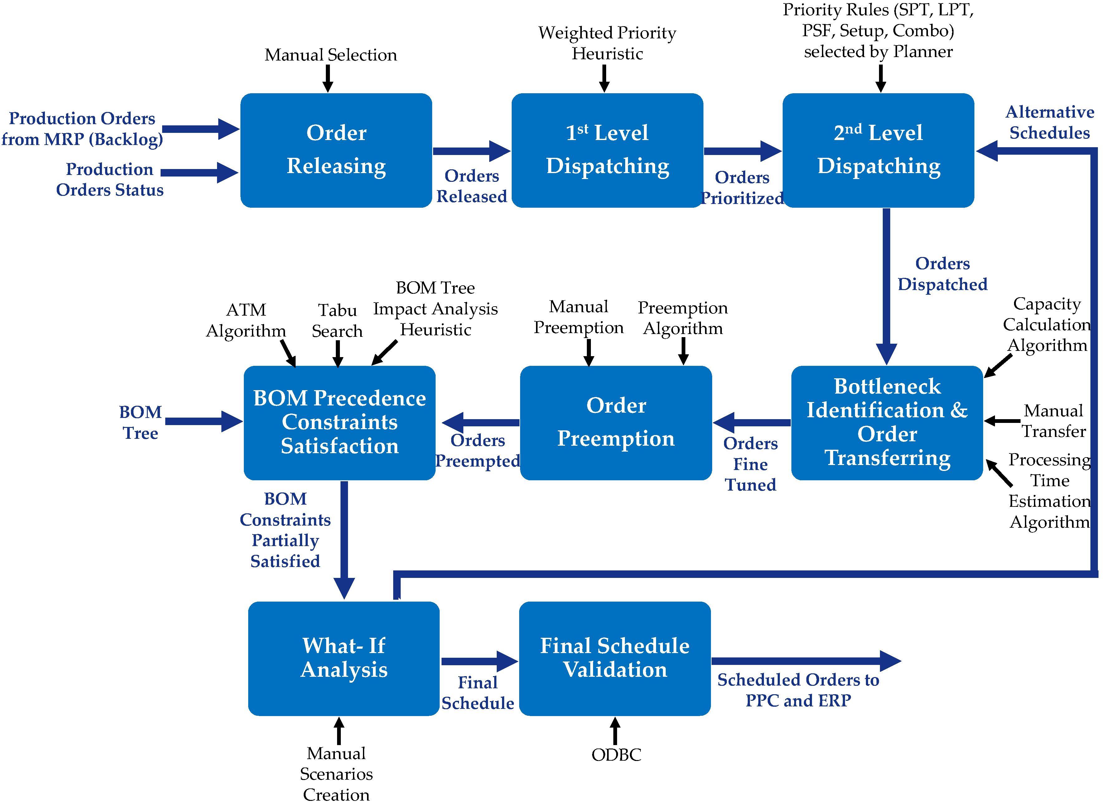Figure 1 summarizes the above process through an activity-based view. The scheduling process is presented as a series of activities, where specific DSS functions support each activity.

The complete functionality of the G-DSS is presented in

Table 3. G-DSS’s functionality and methods.

Functionality	Functionality Type	Methods/Algorithms
Production order and work center data extraction from PPC system	Supplementary	The common database schema, ODBC
Order releasing	Core	Manual selection by planner, automatic inclusion or exclusion of late orders
1st level dispatching	Core	Weighted earliest due date heuristic (WEDD)
2nd level dispatching	Core	Weighted priority dispatching rules: shortest processing time (SPT), longest processing time (LPT), slack, presubcontractor first (PSF), setup, combo)
Schedule representation (supervision of order information, workload and bottleneck work centers)	Supplementary	Gantt chart
Bottleneck identification	Core	Capacity calculation algorithm, Processing time estimation
Order transferring (either to alternative production planning periods or alternative work centers) and Order preemption	Core	Manual input, preemption algorithm
Order transferring in “freeze” mode	Core	Manual input
BOM precedence constraints satisfaction (supervision and control of BOM precedence constraint violation, component availability check and impact estimation of order transferring according to BOM tree)	Core	TS/VNS, BOM tree impact heuristic, ATM algorithm, BOM relationship representation method
What-if analysis	Supplementary	Alternative scenarios management
Construction of final production schedule	Supplementary	Report generation
PPC and ERP database update	Supplementary	Common database schema, ODBC

. Every function is categorized according to its decision support contribution as “core” or “supplementary”. For example, order releasing and dispatching are core decision support functions that assist the planner in performing detailed production scheduling. At the same time, schedule representation and reports are supplementary since they aim to present and validate the decision-making process’s outcome. Furthermore, the various methods and algorithms incorporated by every function are presented in Table 3.

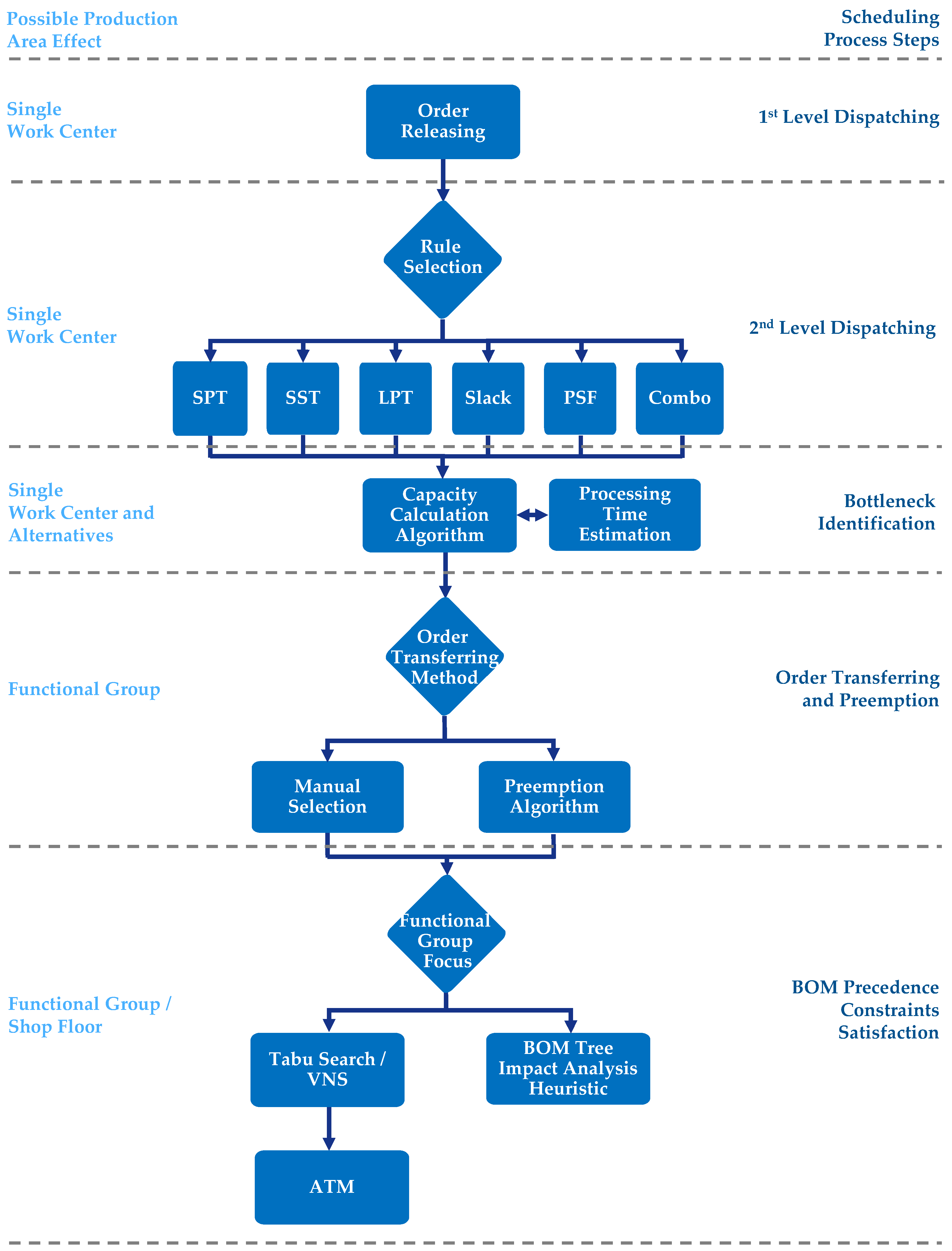
Figure 2 provides a method/algorithmic-oriented view where the sequence of algorithms is provided for each system function of Figure 1. For example, the second-level dispatching function utilizes the prioritized orders of the previous step using an assortment of different priority rules in order to create the dispatched orders. Additionally, from a decision support view, during the second-level dispatching, the planner reaches a node and is called to choose a specific priority dispatching rule while taking into account the area of effect of these heuristics, which in that case, is a single work center. It should be noted that for the final step, i.e., BOM precedence constraint satisfaction, the compound TS/VNS-ATM algorithm has a functional group breadth, whereas the impact analysis heuristic considers the entire shop floor (all the functional groups). The next section thoroughly describes these heuristics and algorithms for the core functionality of the DSS.

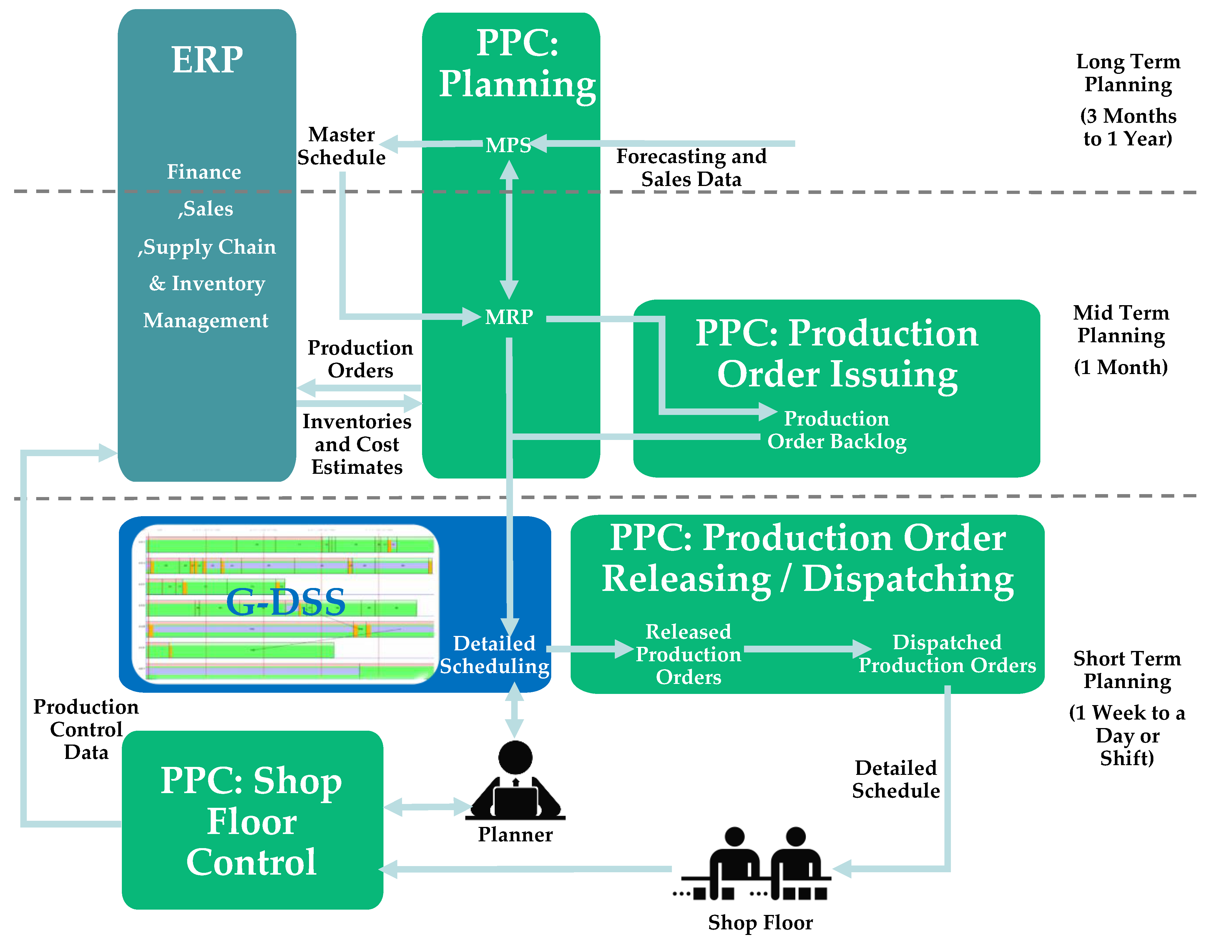
Finally, Figure 3 presents a framework for the G-DSS system that is based on all the operations that were analyzed in Section 2 and Section 3. More specifically, the figure presents the interactions of the three enterprise systems. The production scheduling process starts at the PPC planning module with the MPS calculations that are fed to the MRP. These calculations are based on forecasting and sales data. The ERP provides inventory information (used in MRP) and then receives production and purchase orders (as output from the MRP). It can also provide cost estimates for the orders. The MRP sends orders and order backlog (from the PPC production order issuing module) to the G-DSS for use in detailed scheduling. The G-DSS generates detailed schedules based on the aforementioned data and commands from the planner. The PPC production order releasing/dispatching module helps by releasing and dispatching production orders to the shop floor. This detailed schedule is handed to the shop floor to start production. The PPC shop floor control module aids the process by receiving necessary data from the production and sending them to the planner for analysis. Finally, the process concludes with the PPC shop floor control module sending the production control data to the ERP system.

4. Algorithms for Core System Functionality

4.1. Dispatching Level Heuristics

The heuristics chosen for the dispatching level are PDRs. Due to their approximate nature, they seldom find the optimum solution. However, this has not posed a significant disincentive regarding their practical implementation. Ever since their initial conception through the Giffler–Thompson algorithm [19], PDRs have been used extensively in actual manufacturing environments due in large to the alignment of their mathematical formulation with the shop floor [20]. For example, a worker is capable of easily understanding the concepts of SPT, earliest due date (EDD), and first in first out (FIFO), while those of ant colony optimization and artificial immune system are harder to grasp. Another reason for their wide practical use is their speed in producing schedules: Where a branch and bound technique or a mixed-integer linear programming (MILP) model would have to run for a very large amount of time, PDRs produce schedules in a matter of seconds. This is of huge importance in real industrial situations such as the one highlighted in this paper since unexpected events, such as machine breakdown and rush orders, may, and more often than not, do happen. A new schedule must be constructed on the fly so time-consuming algorithms are avoided.

From a problem-solving perspective and for the efficient application of PDRs, it was deemed preferable to break down the original $n\times m$ problem, where n represents the production orders and m represents the machines, into a series of single-machine $n\times 1$ instances with a common due date, solve them one by one, and then aggregate the partial sequences to construct a full schedule. Precedence constraints between orders are ignored at this stage. The reason for such a decomposition strategy was twofold: Firstly, the order backlog created by the MRP function discretely assigns SKUs to work centers and BOM effectivity dates, and secondly, the large number of orders traversing the shop floor significantly increases problem complexity when concurrently catering for the BOM tree structure. Empirical analysis showed that schedule quality does not considerably improve by solving the constrained $n\times m$ problem, while the computational overhead can be up to 150 times as much. For example, when scheduling the cutting group whose typical problem size can be 201 × 10, aggregation of the $n\times 1$ partial schedules takes, on average, 6s on a low-end 3.10 GHz dual-core system with only 4096 MBs of RAM. In contrast, using a genetic algorithm approach, the/problem took a minimum of 15 min on the same hardware platform. The approach taken was further validated by the production staff that preferred rapid scheduling and rescheduling over close to optimal schedules.

Table 4. Cutting group $n\times 1$ problem instances.

Work Center Code	Active SKUs Spanning Two PPS	Total No. of SKUs	No. of Active Orders Spanning Two PPPs	Total No. of Orders (Including Late)	Maximal Problem Instance
A511	24	62	34	70	70 × 1
A112	20	38	13	33	33 × 1
A111	16	35	16	27	27 × 1
A121	14	31	8	17	17 × 1
A122	13	30	7	31	31 × 1
A131	2	3	2	3	3 × 1
A125	2	2	3	5	5 × 1
A652	1	8	4	8	8 × 1
A654	Not used	3	Not used	5	5 × 1
A653	Not used	6	Not used	2	2 × 1
Total	92	218	87	201	201 × 1

shows how the 201 × 10 instance is broken down into 10 $n\times 1$ problems. It should be noted that in the relevant table, the two production planning periods (PPPs) are chosen randomly. For these two, the active SKUs (according to BOM effectivity dates) are presented, along with the total SKU number (all BOM trees). Columns 4 and 5 depict the production order number without and with late order inclusion. As can be seen, late orders are numerous and significantly overburden scheduling. The main reason for such a large number is the poor performance of the PPC tool, the extensive outsourcing (subcontractors violate due dates), and a sizeable amount of orders with small quantities (two to three components) that accumulate over the year. Another point of interest is the fluctuating number of active SKUs. For the selected PPPs, none of the active SKUs were bound to work centers A654 and A653. If late orders are included, seven new production orders are allocated to those centers, which evince that BOM effectivity dates may overlap, thus further contributing to problem complexity.

The PDRs chosen by the authors to solve the $n\times 1$ problems are shown in

Table 5. PDRs embedded in the G-DSS.

Rule	Order Priority Type	Rank and Priority Index		Best Objective Function Performance
SPT	Shortest processing time	min	$\tau i{m}_i$	Total flowtime
wEDD	Weighted earliest due date	min	$wi\times di$	Max weighted tardiness	$wT\max =\underset{i-1\le i\le n}{\max }wiTi$
SST	Shortest setup time	min	$si{m}_i$	Setup times	$ST={\displaystyle \sum }_{i-1\le i\le n}si{m}_i$
LPT	Longest processing time	max	$\tau i{m}_i$	Total earliness
Slack	Minimum slack remaining	min	$di-ri{m}_i$	Total lateness
PSF	Pre-subcontractor order first	min	$d{i}_{PS}$	Max tardiness of PS orders	$T{\max }_{PS}=\underset{{(i-1)}_{PS}\le i_{PS}\le n_{PS}}{\max }T{i}_{PS}$
Combo	Combination of SPT, PSF, Slack, LPT, SST	min/ max	S(i)	Multi-objective	All the above

. The choice was propagated by interviews with the SME’s production unit staff. The interviews highlighted the objectives most important to the planner and the foremen and are given in column 5 of Table 5, along with their mathematical descriptions. Once the required objectives to be satisfied were established, a thorough literature search was conducted to pinpoint the PDRs best suited to them. These PDRs were EDD, SPT, LPT, SST, minimum Slack, and PSF.

In the first-level dispatching, all the $n\times 1$ problems are solved according to the weighted EDD rule. The due date is common for all on-time orders (end of the current PPP) and negative for the late ones (end of their previous PPP). As such, late orders are ranked first according to their significance level—the weights in the EDD—and the same is performed for the remaining ones. No machine idle time is allowed, since, for the $n\times 1$ case, the optimal schedule utilizes the machine fully.

Second-level dispatching is performed in a similar way, but with the rest of the PDRs in Table 5. Orders are classified and sent in ascending or descending order by SPT and LPT, respectively, based on their processing time. SST tries to group together similar SKUs (late and on time) in order to save setup time and can be strengthened further by selecting whether to schedule orders ascending or decreasing in setup length. There are no settings that are sequence-dependent, and the SME uses an average configuration for each work center. Slack prioritizes orders based on their processing time and due dates in order to avoid late orders. If late orders are not included since all the remaining ones have a common due date, slack is relegated to the LPT rule. Slack may seem redundant at this point, but the SME is planning to break the common due date rule by assigning smaller due dates to pre-subcontractor orders and that was the key driver behind the inclusion. Until the final definition of subcontractor due dates, PSF was included to give priority to the relevant orders by positioning them at the start of the PPP so as to outsource the post-processed components as early as possible.

Thenarasu et al. (2022) [21] noted that combinations of PDRs will almost certainly outperform any simple PDR implementation; a conclusion derived from the high dependency of PDRs on problem-specific knowledge. With that in mind, the authors implemented a template through which the planner can create a combination (combo) of rules by assigning weights to each one. This enables the formulation of a production order sequence $Sm$ that can be easily tweaked to suit a given problem better. The template is given in Equation (1) along with the constraints and possible values of the various parameters.

$$S_m={\displaystyle \sum }_{m_i=1}^{m_i=m}{S}_{m_i}$$

(1)

where

$$\begin{gathered} m_i=\left(w1\times SPT{m}_i+\delta 1\times WEDD{m}_i\right)+\left(w2\times LPT{m}_i+\delta 2\times WEDD{m}_i\right) \\ +\left(w3\times PSF{m}_i+\delta 3\times WEDD{m}_i\right)+\left(w4\left(k\times aSST{m}_i+\left(1-k\right)dSST{m}_i\right) \\ +\delta 4\times WEDD{m}_i\right) \end{gathered}$$

(2)

Subject to:

$$\begin{gathered} w1+w2+w3+w4=1 \mathrm{and} \\ \delta 1,\delta 2,\delta 3,\delta 4=1 \mathrm{for} \mathrm{late} \mathrm{order} \mathrm{prioritization}, \mathrm{else} \\ \delta 1,\delta 2,\delta 3,\delta 4=0 \\ k=0 \mathrm{for} \mathrm{descending} \mathrm{SST} \mathrm{sequence} \left(\mathrm{dSST}\right) \\ k=1 \mathrm{for} \mathrm{ascending} \mathrm{SST} \mathrm{sequence} \left(\mathrm{aSST}\right) \end{gathered}$$

4.2. Bottleneck Identification and Order Transferring Methods

The practical application of the G-DSS showed that second-level dispatching is usually followed by alleviation of the resulting bottlenecks. Due to the accumulation of late orders and violated due dates by the subcontractors, the planned orders by the PPC system may still surpass the capacity of a work center for a full PPP. Bottlenecks are pinpointed using the bottleneck identification method. Using data regarding capacity, order quantities, shifts per day, hours per shift, and efficiency, the G-DSS calculates the workload of a work center via the following function: $WL{m}_i={\displaystyle \sum }_{i=1}^{i=n}\tau i{m}_i$, where ${\tau }_{i{m}_i}=N_i/\left(a{m}_i\times pCapi{m}_i\right)$, with $a{m}_i$ representing the efficiency of the work center $m_i$ and $pCapi{m}_i$ representing the capacity of machine $m_i$ required to produce a unit of SKU $i$ ($a{m}_i$ and $pCapi{m}_i$ are taken from the PPC database). If $WL{m}_i>PPPL{m}_i$, where $PPPL{m}_i=daysppp\times no\_shifts{m}_i\times hrs\_shift$, then $m_i$ is flagged as overloaded and the planner is prompted for action. There are two types of action the planner may take: Either transfer orders to earlier or later PPPs or alternate work centers. In the case of alternate centers, the G-DSS functions in the following manner:

• Calculate the capacity margin of alternate work centers $m_k$, i.e., CMm_k = PPPLm_k − WLm_k.
• If $CM{m}_k>0$ do:
  • Calculate ${\tau }_{i{m}_k}=N_i/(a\times pCapi{m}_k)$.
  • Add ${\tau }_{i{m}_k}$ to $WL{m}_k$.
  • Repeat until $CM{m}_k=0$.

Instead of making the above moves automatically, the G-DSS informs the planner through a form of possible production orders that may be moved to alternate work centers and leaves the end decision up to them.

Except for the typical manual transferring function, the planner may also utilize the “freeze mode”. In “freeze mode”, the planner may transfer production order i to any given point in the sequences $S{m}_i\vee S{m}_l\vee \dots \vee S{m}_k$, with $\left[ml,\dots ,mk\right]$ representing the set of alternate machines, by concurrently inserting machine idle time, which is prohibited during the first and second dispatching levels. This function was employed in the G-DSS mainly to cater for dynamic shop floor events such as machine breakdowns, maintenance, rush orders, etc. For example, if $m_i$ breaks down, then the planner would activate “freeze mode” to insert the necessary idle time in $S{m}_i$ to accommodate the repair time.

4.3. Order Preemption Algorithm

As embedded in the G-DSS, order preemption is applicable to orders that have a delayed status, and a portion of their initial quantity may have already been produced in a previous PPP. If $N{i}_{initial}$ is the initial order quantity of order $i$ and $N{i}_{remaining}$ is the remaining quantity to be produced, then the following steps are performed:

• Create set $P=\{i:N{i}_{initial}-N{i}_{remaining}>0,\forall i\in P\}$ $\forall i\in P$ do:
  • Deem $N{i}_{remaining}$ as the quantity of new production order $i_{remaining}$.
    • Set $PPP{i}_{remaining}=PPPcurrent$ if $CM{m}_i>0$, else.
    • $PPP{i}_{remaining}=PPPcurrent+1$.
  • Assign new production order id for $i_{remaining}$.
  • Set $N{i}_{initial}-N{i}_{remaining}$ as the quantity of production order $i$.
  • Set $PPPi=PPPinitial$.
  • Keep production order id of $i$ for new $i$.
  • Set order status of $i$ as closed.
• Terminate.

In addition to the above algorithm, the planner can also perform manual preemption by selecting the orders they wish from the P set and setting the desired $N{i}_{remaining}$ quantities. The scope of preemption is twofold: To alleviate bottlenecks and overloaded work centers by preempting orders for centers with $CM{m}_i<0$ and compare the PPC-planned production quantities with the quantities actually produced at certain PPPs.

4.4. BOM Precedence Constraint Satisfaction Metaheuristics

The first- and second-level dispatching methodologies outlined in Section 3.1 ignore, in favor of speed, precedence constraints that may exist among components scheduled to be produced within the same PPP. Except for scheduling speed, the main reason for this decomposition strategy was the make-to-stock policies the SME employs for raw materials, components, and end items. If there is sufficient stock of a child (the preceding component) to initiate production of the father (the succeeding component), then this type of precedence relationship can be regarded as a soft constraint with the penalty being the child’s stock reduction. Due to the nature of the PPC system, it is an extreme rarity to come across more than a single-level child–father occurrence in a PPP, e.g., $i-1\to i\to j$ where $i-1$ and $i$ denote the child and father/child, respectively, and j represents the father. Therefore, in the remainder of the paper, the focus will be solely on $p\left(i,j\right)$ pairings.

The authors, in order to explore the feasibility of a schedule with precedence constraint violations, formulated a hybrid TS/VNS algorithm coupled with the ATM module already mentioned in the paper. For more information regarding TS and VNS, the reader is referred to Qiu et al. (2018) [22] and Rezgui et al. (2019) [23], respectively. In this unique implementation, random weights are assigned to SPT, LPT, and PSF, and a typical TS algorithm with backtracking is executed. The neighborhood consists of $\pm 0.02$ of the previous iteration’s $w1,w2,w3$ values. Two tabu lists are kept to store the values of $w1,w2,$ with $w3=1-w1-w2$. If a neighbor is found in which either $w1$ or $w2$ belong in the respective tabu lists, then that neighbor is rejected. Solution quality is determined by the number of properly oriented $p\left(i,j\right)$ pairings, i.e., $Ci\le rj$.

Two additional counters are initiated: $vns\_counter=0$ and $cycle\_counter=0$. These counters count the number of iterations for which the current solution quality has not improved. Once the $vns\_counter$ reaches a certain number of iterations, the VNS concept of shaking is applied to launch $w1$ and $w2$ into other neighborhoods and diversify the search. If shaking fails to improve the quality and the $cycle\_counter$ fill-up search up to that point stops, an elite solution is chosen from the elite set, the tabu lists are wiped, and the search is reinitiated from this solution. The elite set holds a number of promising solutions found during search and ranks them in last in first out (LIFO) fashion, thus serving a number of good points for re-intensification when the search stagnates. The search terminates when all possible pairings have been properly oriented, all possible elite solutions have been used, or the maximum number of iterations has been exhausted. The pseudocode of the algorithm is the following:

• Initialize parameters of the TS/VNS algorithm.
• Assign random weights $w1,w2,w3$ to SPT, LPT, PSF and set $iters=0$, $tabu\_list1=0$, $tabu\_list2=0$.
• $\mathrm{If} \mathrm{late} \mathrm{orders} \mathrm{are} \mathrm{prioritized} \mathrm{then} \delta =1,$
  $\mathrm{Else}\delta =0$.
• Create elite set $E=\left\{u\left(w1,w2,n\left(n^{+}\right)\right)\right\}$ with $n\left(E\right)=8$ and set $vns\_counter=0$, $cycle\_counter=0$.
  • Create a sequence for which the following holds true: $S=w1\times SPT+w2\times LPT+w3\times PSF+\delta \times WEDD\wedge w1+w2+w3=1$.
  • Calculate $n^{+}=\{p\left(i,j\right)\in n^{\max }:S^{-1}\left(i\right)<S^{-1}\left(j\right)\}$.
  • Add current $\left\{u\left(w1,w2,n\left(n^{+}\right)\right)\right\}$ to E.
  • Locate non-tabu neighbor of S, S* by randomly perturbing $w1,w2$ within a $\pm 0.02$ interval (neighborhood), set $w3=1-w1-w2$.
  • Calculate $n^{+}=\{p\left(i,j\right)\in n^{\max }:S^{-1}\left(i\right)<S^{-1}\left(j\right)\}$.
  • If $n\left(n_{S^{*}}^{+}\right)>n\left(n^{+}\right)$ set S = S* and add $w1,w2$ to $tabu\_list 1$ and $tab{u}_{list2}$ and set $iters=iters+1$.
  • If $n\left(n_{S^{*}}^{+}\right)>n\left(n_{\min }^{+}\right),n\left(n_{\min }^{+}\right)=\min n\left(n^{+}\right),\forall u\in E$ then replace $u_{\min }$ with $u_{S^{*}}$ and set $vns\_counter=0$, $cycle\_counter=0$.
  • If $n\left(n_{S^{*}}^{+}\right)\le n\left(n_{\min }^{+}\right),n\left(n_{\min }^{+}\right)=\min n\left(n^{+}\right),\forall u\in E$ then set $vns\_counter=vns\_counter+1$, $cycle\_counter=cycle\_counter+1$.
  • If $vns\_counter=60$ perform shaking by randomly setting $w{1}^{*}=w1\pm 0.1\wedge w{2}^{*}=w2\pm 0.1$.
  • If $cycl{e}_{counter}=75$ then recover $u_{lifo}\left(w1,w2,n\left(n^{+}\right)\right)$ and set $w1=w{1}_{lifo}$, $w2=w{2}_{lifo}$ and go to a.
• Terminate if $n\left(n^{\max }\right)=n\left(n^{+}\right)\vee n\left(E\right)=\varnothing \vee iters=\max iters$.

Empirical analysis showed that in the vast majority of the cases, the TS/VNS algorithm did not properly orientate all the $p\left(i,j\right)$. This outcome was of no surprise since no problem-specific knowledge is incorporated into the algorithm. Furthermore, such a result does not necessarily create an infeasible schedule, as was previously mentioned. To test schedule feasibility, the ATM algorithm is employed. Once its parameters are initialized, ATM identifies a set of $p\left(i,j\right)$ pairings that maintain improper orientations and then proceeds to create three discreet subsets: Subset C contains pairings in which children have 1 to 1 relationships with the fathers, subset F contains pairings of n to 1 type relationships, and finally, subset K, in which those same relationships are 1 to n. The next step is the calculation per subset of the earliest possible starting times $\min rj{m}_j$ of the fathers while taking into account current stock levels, desired child quantities, and children’s completion times. Comparisons of these starting times with the ones provided by the TS/VNS algorithm reveal if feasibility has been broken. The steps of ATM are given below:

• Initialize ATM parameters.
• Identify set $n^{-}=\left\{p\left(i,j\right)\in n^{\max }\backslash n^{+}\right\}$.
• Dim $C=\left\{p\left(i,j\right)\in n^{-}:i\ne k,j\ne l,\forall p\left(i,j,\right),p\left(k,l\right)\in C\subseteq n^{-}\right\}$.
  • If $mj=mi$ then δ$mjmi=0$, else δ$mjmi=1$.
  • $\forall p\left(i,j\right)\in C$ calculate $\min rj{m}_j=ri{m}_i+\delta m_i{m}_j\times \tau i{m}_i\times \left(1-\frac{STi}{Ni}\right)+\left(1-\delta m_i{m}_j\right)\times \tau i{m}_i$.
  • If $rj{m}_j<\min rj{m}_j$ then the orientation of $p\left(i,j\right)\in C$ is wrong.
• Dim $F=\left\{p\left(i,j\right)\in n^{-}\backslash C:j\ne l,\forall p\left(i,j,\right),p\left(k,l\right)\in F\subseteq n^{-}\right\}$.
  • $\forall j\in F$.
    • $\forall i\in F$ calculate $\min rj{m}_j=ri{m}_i+\delta m_i{m}_j\times \tau i{m}_i\times \left(1-\frac{STi}{Ni}\right)+\left(1-\delta m_i{m}_j\right)\times \tau i{m}_i$.
  • Find $\max \left(\min rj{m}_j\right)$.
  • If $rj{m}_j<\max \left(\min rj{m}_j\right)$ then the orientation of $p\left(i,j\right)\in F$ is wrong.
• Dim $K=\left\{p\left(i,j\right)\in n^{-}\backslash C:i\ne k,\forall p\left(i,j,\right),p\left(k,l\right)\in K\subseteq n^{-}\right\}$.
  • $\forall i\in K$.
    • $\forall j\in K$ calculate $\Delta =rj{m}_j-\left(ri{m}_i+\tau i{m}_i\right)$.
      • For $mi=mj$ if $\Delta <0$ then the orientation of $p\left(i,j\right)\in K$ is wrong.
      • For $mi\ne mj$ then
        • $\forall p\left(i,j\right)\in K\wedge \Delta <0$ if $STi\le {\displaystyle \sum }_{j=1}^{J}N{i}_j$ then at least one of $p\left(i,j\right)\in K$ the orientations are wrong.
        • $\forall p\left(i,j\right)\in K\wedge \Delta >0$ then $p\left(i,j\right)\in K$ is correctly oriented.
• Collect all wrongly oriented $p\left(i,j\right)\in n^{-}$ and terminate.

ATM’s termination is accompanied by the feasibility status of the schedule. Empirical data showed that infeasibility is highly probable, especially for functional groups with a very large number of $p\left(i,j\right)$ pairings (as many as 60 spanning two PPPs), such as door lock assembly. If that is the case, the next step is supporting the planner in his decision to properly orientate the wrong pairs through the repair method outlined below:

• $\forall p\left(i,j\right)\in C^{-}$ do:
  • Prompt user to transfer either $i$ or $j$ earlier or later until $rj{m}_j=\min rj{m}_j$.
• $\forall p\left(i,j\right)\in F^{-}$ do:
  • Prompt user to transfer either $i$ or $j$ earlier or later until $rj{m}_j=\max \left(\min rj{m}_j\right)$.
• $\forall p\left(i,j\right)\in K^{-}$ do:
  • Calculate all $\frac{\tau j{m}_j}{N{i}_j}$.
  • Find $j$ with $\min \frac{\tau j{m}_j}{N{i}_j}$.
  • Prompt user to transfer $j$.
  • If $STi\ge {\displaystyle \sum }_{j=1}^{J}N{i}_j$ terminate, else go to b to find next $j$.

Of final note in this section is the impact analysis heuristic. This heuristic extends the logic behind BOM precedence constraint satisfaction to all the functional groups. Execution normally comes after the termination of the TS/VNS-ATM algorithm for all functional groups. The first step is the identification of $p\left(i,j\right)$ pairings for which $i$ and $j$ belong to different functional groups. For all such pairs, if transferring or any type of dispatching has led to $PPPi=PPPj$, hence $i$ has been delayed, then the planner is prompted to transfer $j$ to $PPPj=PPPi+1$.

Additionally, if $i$ has been moved significantly earlier (a rare occurrence), for example, $PPPi=PPPj-3$, then the planner is prompted to transfer $j$ to $PPPj=PPPj-2$. The main goal is to have a single PPP difference for all pairs belonging to different functional groups, thus conforming to the lead times. The exhortations are presented to the planner via a report indicating the child–father production order codes, the work centers producing them, their respective functional groups, the start and finish times, and finally, the PPPs.

Table 6. Synopsis of core functionality algorithms.

Algorithm	Inputs	Outputs
Weighted earliest due date heuristic (WEDD)	Quantities, processing times, due date, priority level	Sequence of orders
Priority rule “SPT”	Quantities, processing times, due date	Sequence of orders
Priority rule “LPT”	Quantities, processing times, due date	Sequence of orders
Priority rule “PSF”	Quantities, processing times, due date	Sequence of orders
Priority rule “SST”	Quantities, processing times, due date, setup times per workcenter	Sequence of orders
Priority rule “Combo”	Quantities, processing times, due date, setup time, priority level	Sequence of orders
Capacity calculation algorithm	Work center capacity, quantities of sequenced orders	Work centers load, bottleneck identification
Processing time estimation algorithm	Alternative work centers, capacities, quantities of sequenced orders	Processing time for alternate work centers
Preemption algorithm	Planned quantities, remaining quantities, due date	New production orders for the remaining quantities
ATM	BOM tree, quantity of “father items”, inventory of “children items”, starting time of “children items”	Production orders of “father items” capable to manufacture
TS/VNS	Weighted priority indexes of priority rules, quantities, processing times, due date, priority level	Improved sequence of orders
BOM tree impact analysis heuristic	BOM tree, due dates, production groups of “father items” and “children items”	List of proposed orders transfers

provides a synopsis of the algorithmic framework presented in Section 4. All the algorithms are presented along with their inputs and outputs. The inputs are directly drawn by the G-DSS from the PPC database since both systems share a common database schema. The only exception is the ATM algorithm where the children’s stock quantities are taken from the ERP system, which functions as the inventory monitoring system of the case study.

5. Computational Results for the TS/VNS-ATM Algorithms

Table 7. Results of TS/VNS-ATM with late orders released.

Functional Group	Late Orders Released
Two PPPs	Total Orders	Father Child Pairings	TS/VNS δ = 1	TS/VNS δ = 0	SPT		LPT		PSF		ATM Result
Intermediate Phases	63	18	8/18 (34 s)	12/18 (32 s)	3	23	96	74	1	3	6/10	3/6
Cylinder Components	65	33	20/33 (37 s)	23/33 (36 s)	33	51	9	34	58	15	9/13	7/10
Seizure and Nailing	48	18	9/18 (29 s)	11/18 (27 s)	29	14	30	31	41	55	5/9	4/7
Cutting	145	24	7/24 (75 s)	12/24 (72 s)	14	32	45	34	41	34	10/17	7/12
PROTON Assembly	10	2	2/2	2/2 (8 s)	19	24	57	62	24	14	------	------
Door Lock Assembly	138	48	17/48 (94 s)	35/48 (89 s)	50	53	8	15	42	32	23/31	10/13
Casting	119	24	9/24 (85 s)	17/24 (82 s)	5	14	74	60	21	26	6/15	3/7

and

Table 8. Results of TS/VNS-ATM with late orders not released.

Functional Group	Late Orders Not Released
Two PPPs	Total Orders	Two PPPs	Total Orders	Two PPPs	Total Orders		Two PPPs		Total Orders		Two PPPs
Intermediate Phases	63	18	8/18 (34 s)	13/18 (32 s)	3	23	96	74	1	3	6/10	3/6
Cylinder Components	63	33	21/33 (35 s)	24/33 (34 s)	27	51	15	34	58	15	10/12	8/9
Seizure and Nailing	48	18	9/18 (29 s)	11/18 (27 s)	29	14	30	31	41	55	5/9	4/7
Cutting	78	12	4/12 (61 s)	7/12 (55 s)	47	34	41	45	12	21	5/8	3/5
PROTON Assembly	10	2	2/2	2/2 (8 s)	19	24	57	62	24	14	------	------
Door Lock Assembly	100	39	11/39 (54 s)	28/39 (50 s)	50	26	5	19	45	64	24/28	9/11
Casting	106	13	12/13 (76 s)	13/13 (72 s)	9	21	69	55	22	24	1/1	-----

present the best results over 20 runs of the hybrid TS/VNS and the complementary ATM module. The algorithms were coded in VB.NET and were run on a low-end 3.10 GHz dual-core system with 4096 MBs of RAM. The parameter settings of the TS/VNS algorithms were maxiters = 10,000, n(E) = 8, tabu_list1 = 6, tabu_list2 = 6, vns_counter = 60, cycle_counter = 75. The same two random sequential PPPs were chosen for all functional groups, and two sets of experiments were conducted. In the first (Table 7), the late orders accumulated over the course of the previous PPPs were included, whereas in the other (Table 8), they were not released for dispatch. This approach highlighted one interesting aspect regarding the shop floor mentality of the case study leading up to the G-DSS implementation: Functional groups such as seizure and nailing and intermediate phases may have as little as 0 late orders, while casting, assembly, and cutting have as many as 38. Additional computational results showed that for the former groups, 0 late orders are neither a rarity nor the norm, ergo it just so happened that for the two PPPs chosen, no late orders had accumulated. For statistical reasons, the end results are presented solely for those two periods.

The tables show the functional group, the total number of orders and $p\left(i,j\right)$ pairings, and the number of correct orientations achieved by TS/VNS with the running time given in the brackets. Two executions of TS/VNS are performed: In the first, parameter δ is set to 1, i.e., late orders due to the first- or second-level dispatching are prioritized, and in the second, δ = 0. The next three columns show the percentages (weights) with which each PDR participates in the best synthesis of rules for each execution. The final column depicts the ATM results. No ATM runs were performed if TS/VNS reached the optimum number of proper $p\left(i,j\right)$ orientations. The maximum running time of ATM was 9 s, and due to this very small value, running times are not included.

At first glance of the results, what becomes apparent is the strong effect δ has on the solution quality. If late orders stemming from initial dispatching, even if previous PPP late orders are not released, are prioritized, then fewer pairs will be properly oriented. Since no machine idle time is allowed during schedule construction, a late order would be scheduled first in a work center compared to a child, whose father may be constrainedly first on its relative work center if no other orders are present. Therefore, this $p\left(i,j\right)$ pair could become wrongly oriented. The same applies if there are additional orders in the father’s work center, but their cumulative processing time is insufficient to surpass both the late orders and the child’s time. This was particularly evident in the cutting group where the capacity of work center A511 (see Table 4) is sizeable, leading to a very large number of short production orders.

In general, if late orders are not released (Table 8), TS/VNS performs slightly better, see for example, the assembly group, but the overall average performance is similar. This leads to another interesting conclusion: The majority of late orders from previous PPPs constitute a child whose father or fathers are on the current PPP. When released immediately, an additional $p\left(i,j\right)$ is identified. If late orders had no correlation whatsoever with the remaining ones, then the performance of TS/VNS would degrade, especially for δ = 1, since late orders occupy additional potential slots that could be used for proper orientation.

The computational overhead of the TS/VNS module is correlated with the number of production orders released and not the total number of $p\left(i,j\right)$ pairs. Overall running times are shallow and can be considered substantial only for the door lock assembly group and the casting phase. No clear conclusions can be drawn regarding the superiority of any single PDR in any group. Apparently, a general pattern can be identified for all functional groups. For example, in the casting phase, δ = 1 LPT appears to perform remarkably well, whereas PSF comes in second, and SPT notes the worst performance of the 3. If δ = 0, the values of $w1,w2,w3$ do not change significantly, but the contribution of SPT increases. Indexes appear to be genuinely stochastic only in the cutting group, while $w1,w2,w3$ appear to be entirely differentiated between Table 7 and Table 8.

The performance of the ATM module validates the approach taken by the authors in tackling this scheduling problem. In most cases of $p\left(i,j\right)$ pairs, there is enough stock of $i$ to commence production of $j$ with the starting time $rj{m}_j$ defined by the TS/VNS algorithm. The maximal number of wrongly oriented $p\left(i,j\right)$ is 8 and is found in the assembly group if late orders are released. The vast amount of orders traversing this group makes additional order transferring by the planner inevitable in order to fully satisfy the BOM precedence constraints. In the other groups, minor adjustments need to be made in the TS/VNS schedule since, in most cases, an average number of 4 $p\left(i,j\right)$ orientations necessitate fixing. The parameter δ has a substantial impact on the ATM output, and this can be seen in both tables. If δ = 1, more children are scheduled later than their relative fathers’ minimum starting time. Empirical analysis showed that the number of wrong $p\left(i,j\right)$ orientations is equal to the respective number if δ = 0, plus the additional disoriented pairs that resulted when prioritization was given to late orders ensued by first and second-level dispatching.

6. Discussion

Consumer desire for variety, shorter product life cycles, changing markets due to global competition, and fast development of new goods, services, and processes have all boosted interest in comprehensive production scheduling among academics and industry. The aforementioned economic and social market constraints highlight the need for a production planning system that requires little inventory, reduces waste output, and maintains customer satisfaction by delivering the right product to the right consumer at the right time. As a result, manufacturing processes such as make-to-order, cellular manufacturing, group technology, demand management, and engineering-to-order have emerged during the previous three decades. Except for process reengineering, different plant layouts, and a reinvented business culture, all of these processes need the facilitation and control of efficient, effective, and precise scheduling. Due to the complexity of scheduling in all but the smallest production facilities, it remained jolted until the mid-1990s, when the first APS systems were launched. These systems integrate operational research algorithms and decision support tools to optimize the whole supply chain, not just the shop floor. Although once hailed as the preferable method for resolving scheduling challenges, their high purchase prices, many installation hurdles, and limited connection with ERP systems rendered them too expensive for the majority of SMEs.

Following that, customized, comprehensive production scheduling DSS systems emerged as a trend. These systems are capable of effectively depicting the unique characteristics of a manufacturing process and are not encumbered by the functionality of typical APS systems. That was also the objective of the research effort described in the paper: To create and implement a customized scheduling DSS in a repetitive make-to-stock SME. While the case study does not use customer-oriented manufacturing processes such as make-to-order, the significant use of subcontractors, the existence of dynamic events, and the piling of late orders highlight the need for shop floor visibility and control.

The requirements were satisfied by the G-DSS releaser/dispatcher, which incorporates all of the essential features and techniques for swiftly producing schedules and makes them accessible through a user-friendly, aesthetically attractive Gantt chart-based GUI. The decision-support part of the system was emphasized through manual selection in order releasing, transferring, preemption, report creation, what-if analysis, and alternative scenario management. The system’s interoperability with the surrounding IT infrastructure, specifically the PPC system and the ERP package, is fully supported, allowing for unhindered information flow through a three-tier planning framework that begins with the calculation of end item requirements over the long term, progresses to disaggregation of those requirements over the medium term, and finally collapses to component and material requirements for a single day or shift via the G-DSS.

The algorithmic framework embedded in the G-DSS enhances decision support functionality by containing all the necessary heuristics, metaheuristics, and methods necessary to facilitate efficient scheduling and full workload control in a complex make-to-stock manufacturing environment with a high order-to-machine ratio, parallel work centers, integrated BOMs and routings, and extensive outsourcing. Dispatching is performed on a single machine level via fast and effective PDRs, and workload control uses manual input supported by proposed preemptions and the utilization of parallel machines. Finally, BOM tree constraints are handled by the hybrid TS/VNS-ATM metaheuristics. Due to this assortment of tools and algorithms, the scheduling process is initiated in a single functional group by selecting the appropriate orders from the backlog and releasing them to the shop floor. First- and second-level dispatching solves the numerous single-machine problems present in the group and feed the remaining steps in order for the schedule to be further improved. Once the work center load has been regulated to below 100%, the child–father pairings are partially satisfied, and the end schedule is validated by updating the PPC and ERP databases.

7. Conclusions

This research provided a procedural sequence for a hierarchical planning framework and included a case study in which the MPS estimated long-term end-item requirements and passed those requirements to the PPC system, which generated the production order backlog. Orders were freed from the backlog and dispatched to work centers, and detailed schedules were prepared using the G-DSS. Generally, a planner will run the G-DSS at the start of each planning period (which is typically a week), extracting the most recent production order data. Schedules may be prepared for each product category and sent to foremen to start production. If dynamic events occur, such as a rush order, a machine breakdown, or a subcontractor fails to meet a deadline, the planner may rearrange to accommodate. The whole procedure is repeated weekly.

As demonstrated in the case study, the SME benefited by gaining visibility into its manufacturing process, reducing lead times, avoiding stock-outs, increasing flexibility and responsiveness to demand fluctuations, and collaboratively organizing its production, maintenance, sales, and procurement departments.

The aforementioned framework is scalable and applicable to similar production make-to-stock environments with few modifications required. Additionally, due to the effectiveness of the TS/VNS-ATM metaheuristic, these environments can benefit significantly from the G-DSS in terms of stock management and utilization. For example, the SME presented in the paper had accumulated component stock by the end of 2021 in the vicinity of 2,000,000 euros. Projected estimates for this year decrease that amount to 1,200,000 thanks to the implementation of the new system.

Applicability of the new production scheduling system is also feasible in make-to-order environments where scheduling speed is of even greater importance. The method of working would be precisely the same, i.e., solving single-machine problems with PDRs and managing constraints with a similar template to the TS/VNS-ATM metaheuristic; however, with alternate stock functions employed. Instead, for such types of shop floors, ATM can be converted into a fully functioning ATP providing the customer with a quick and immediate reply regarding the potential satisfaction of his order. In this light, to gain the full benefit of the G-DSS as a whole, a three-tier planning architecture initiated from aggregate plans and resulting in detailed schedules is best suited.