Article

Efficient 0/1-Multiple-Knapsack Problem Solving by Hybrid DP Transformation and Robust Unbiased Filtering

by
Patcharin Buayen
* and
Jeeraporn Werapun
Department of Computer Science, Faculty of Science, King Mongkut’s Institute of Technology Ladkrabang, Bangkok 10520, Thailand
*
Author to whom correspondence should be addressed.
Algorithms 2022, 15(10), 366; https://doi.org/10.3390/a15100366
Submission received: 16 August 2022 / Revised: 23 September 2022 / Accepted: 27 September 2022 / Published: 30 September 2022
(This article belongs to the Section Combinatorial Optimization, Graph, and Network Algorithms)

Abstract

:
The multiple knapsack problem (0/1-mKP) is a valuable NP-hard problem involved in many science-and-engineering applications. In current research, there exist two main approaches: 1. the exact algorithms for the optimal solutions (i.e., branch-and-bound, dynamic programming (DP), etc.) and 2. the approximate algorithms in polynomial time (i.e., Genetic algorithm, swarm optimization, etc.). In the past, the exact-DP could find the optimal solutions of the 0/1-KP (one knapsack, n objects) in O(nC). For large n and massive C, the unbiased filtering was incorporated with the exact-DP to solve the 0/1-KP in O(n + C′) with 95% optimal solutions. For the complex 0/1-mKP (m knapsacks) in this study, we propose a novel research track with hybrid integration of DP-transformation (DPT), exact-fit (best) knapsack order (m!-to-m2 reduction), and robust unbiased filtering. First, the efficient DPT algorithm is proposed to find the optimal solutions for each knapsack in O([n2,nC]). Next, all knapsacks are fulfilled by the exact-fit (best) knapsack order in O(m2[n2,nC]) over O(m![n2,nC]) while retaining at least 99% optimal solutions as m! orders. Finally, robust unbiased filtering is incorporated to solve the 0/1-mKP in O(m2n). In experiments, our efficient 0/1-mKP reduction confirmed 99% optimal solutions on random and benchmark datasets (n δ 10,000, m δ 100).

1. Introduction

Presently, a variety of NP-hard problems are involved in many real-world applications and AI computing. Solving specific NP-hard problems (with high performance in efficient time) for those applications is challenging. Some of the interesting NP-hard problems are the 0/1-KP (knapsack problem), the 0/1-mKP (multiple m knapsacks), etc.
Formally, the 0/1-KP is defined as follows: Consider a set of n objects and a knapsack capacity C, where each object j (=0, 1, …, n − 1) has profit pj and weight wj.
The objective of the 0/1-KP is to select some objects for the maximum total profit kept in the knapsack that cannot exceed the knapsack capacity (C), defined in Equations (1)–(3). Recently (2018), unbiased filtering [1] was proposed (for the 0/1-KP) to select outstanding objects (from n objects) before applying the exact DP (dynamic programming) algorithm on small remaining n′ (≤200) in efficient time for most optimal solutions (at least 95%) of regular and irregular datasets.
Maximize   j = 0 n 1 p j x j
Subject   to   j = 0 n 1 w j x j   C
and xj ∈ {0, 1}; j = 0, 1, 2, …, n − 1
For the complex 0/1-mKP (m knapsacks), the objective is to select some objects for multiple knapsacks (each selected object j (xij = 1) in a proper knapsack i) that cannot exceed each of the knapsack capacities (Ci; i = 1, 2, 3, …, m), see Figure 1 (one and m knapsacks), for the maximized total profit, defined in Equations(4)–(6).
Maximize   i = 1 m j = 0 n 1 p j x i j
Subject   to   j = 0   n 1 w j x i j   C i   ;   i = 1 ,   2 , ,   m ;   j = 0 ,   1 ,   2 , ,   n 1
and   i = 1   m x i j   1 ,   x i j     { 0 ,   1 } ;   i ,   j
The 0/1-KP and 0/1-mKP are constructive for science and engineering applications, such as resource allocation [2,3], capital budgeting [4], production planning [5], multicontainer packing [6], risk balancing and assortment optimization [7], other applications in network systems [8,9,10], etc. However, finding the optimal solution of the 0/1-mKP is much harder than that of the 0/1-KP since each selected object (xij = 1) must specify a proper knapsack (Ki with capacity Ci; i ∈ {1, …, m}) from the available knapsacks.
In popular 0/1-KP research, two approaches are extensively studied: 1. the exact approach for optimal solutions (but in exponential time) and 2. the fast approximate approach (but the optimal solution may not be found). In theory, the optimal solution of the 0/1-KP can be computed by DP (dynamic programming) algorithms in O(nC) [11,12,13,14,15], or BnB (branch-and-bound) [16] and backtracking [17] algorithms in exponential time (O(2n)). In practice, approximate methods (i.e., greedy methods [18,19], kernel search [20,21], genetic algorithms [22,23], swarm optimization [24,25,26,27,28], hybrid methods [29,30,31,32], hyper-heuristic method [33], etc.) can find the good solutions in polynomial time. Recently, the time-space reduction algorithm [1] was proposed to solve the 0/1-KP in O(n + C′) for large n by unbiased filtering to preselect the outstanding objects (from n objects) before applying the exact DP algorithm on remaining n′ and C′ (n′ ≤ 200, C′ << C, and massive C may not be a polynomial bound of n), which could find most optimal solutions (at least 95%) in experiments.
In current KP-researches, a variety of 0/1-KPs have been studied, including the multiple KP (0/1-mKP) [34,35,36], no shared xij in m knapsacks ( j = 0   n 1 w j x i j   C i ), the multidimensional KP (0/1-MKP) [37,38,39,40,41], ( i = 1 m j = 0 n 1 w i j x j   C i shared xj in m knapsacks), and the multidimensional multiple-choice KP (0/1-MMKP) [42]. However, the exact solutions of those complex KPs could not be easily found on large n. Recently, the mathematical HyMKP [34] was proposed in O(mnC) for the 0/1-mKP with most optimal solutions (in τ s) on n ≤ 500. For large n and massive C, the existing meta-heuristic algorithms for the 0/1-KP can be applied to solve the 0/1-mKP in polynomial time (but requiring the proper knapsack orders). For high performance, the exact DP could find the optimal solution of the 0/1-KP in O(nC) and O(m!nC) for the 0/1-mKP (with m! orders, C = max(Ci)) for at least 99% optimal solutions (but for small m, n, and C). In this study, we are interested to solve the 0/1-mKP for large m, n, C with the proper orders in efficient time. Our hypothesis is “For each of m knapsacks, apply unbiased filtering before using the exact DP on remaining n′ and Ci’ can find most optimal solutions in efficient time”.
In this research, we introduce a novel research track (a hybrid approach of time-space reduction) for solving the 0/1-mKP in efficient time with expected 99% optimal solutions. In our hybrid approach, we propose the integration of DP transformation (reducing C to C’), exact-fit (best) knapsack-order (reducing m! to m2), and 3. robust unbiased filtering (for polynomial time). First, we propose the DP transformation (DPT) algorithm to find the optimal solutions of the 0/1-KP (for each of m knapsacks) in O([n2, nC]), or O(n2) in the best case and O(nC) in the worst case, before being applied for m knapsacks. Second, for the 0/1-mKP (m knapsacks), we propose the exact-fit (best) knapsack order (in our multi-DPT) in O(m2[n2, nC]) for achieving the good solutions as m! orders (at least 99% optimal solutions). Third, robust unbiased filtering is incorporated to solve the 0/1-mKP in polynomial time (O(m2n)) while retaining 99% optimal solutions. The correctness and complexity of the DPT and multi-DPT algorithms are analyzed. In experiments, the original multi-DPT and the multi-DPT + robust unbiased filtering are evaluated on random and benchmark datasets (n ≤ 10,000, m ≤ 100).
The main parts of this paper are organized as follows: Section 2 reviews the related work. Section 3 presents the DPT algorithm to find the optimal solutions of the 0/1-KP in O([n2, nC]). Section 4 proposes the multi-DPT algorithm with the exact-fit (best) knapsack order to solve the 0/1-mKP in O(m2[n2, nC]) and reduced to O(m2n) by our robust unbiased filtering. Section 5 provides the algorithm analysis (correctness and complexity). Section 6 performs the experiments to evaluate the performance of our multi-DPT algorithm and robust unbiased filtering. Section 7 concludes this study.

2. Related Work

For 0/1-mKP research, finding most optimal solutions (≥99% optimal performance) in an efficient time is challenging. First, Section 2.1 reviews the exact DP algorithms to find the optimal solutions of the 0/1-KP. Section 2.2 explores the time-space reduction algorithm to solve the 0/1-KP in polynomial time. Section 2.3 reviews the recent QDGWO (quantum-inspired differential evolution with adaptive grey wolf optimizer) for the 0/1-KP. Section 2.4 explores the efficient mathematical HyMKP model for the 0/1-mKP.

2.1. 0/1-KP Solving by Dynamic Programming Algorithm

For 0/1-KP solving, let tp[C] be an array of total profits, soltp be a maximum total-profit, soltw be a total-weight (≤C), and solx[n] be an array of solution X (xj = 0/1). Algorithm 1 presents the basic DP [11] with two functions (preprocessing and X-tracking on a 2D array or a matrix (n × C)) to find the optimal solution (soltp, soltw, solx[n]) in O(nC). For example, consider n = 6, C = 18, P = {42, 39, 38, 37, 35, 38}, and W = {10, 11, 11, 8, 10, 9}, Figure 2 displays the result of preprocessing (soltp = 79) and X-tracking (solx = {1, 4} from soltp = 79) by applying Algorithm 1. However, using the 2D array (n × C) reserves a huge space, which is not practical if C > n2. Thus, the fast DP (Algorithm 2) [11] uses a 1D array (of C elements) to find soltp in O(nC) but without solx[n] since the 1D array of the last tp-result cannot support the X-tracking (for all selected objects). Finally, the complete DP (Algorithm 3) [11] (p. 24) uses a 1D array for the full optimal solution (soltp, soltw, solx[n]) by repeating the fast DP (for k selected objects) in O(knC).
Algorithm 1: Basic DP with 2D array (for soltp, soltw, solx[n]) in O(nC).
  •  for (d = 0 to C) tp [0,d] = 0;
  •  for (j = 1 to n) do         // preprocessing for soltp
  •   for (d = 0 to wj−1) tp[j,d] = tp[j − 1,d];
  •   for (d = wj to C) do
  •    if (tp[j − 1,d-wj] + pj > tp[j − 1,d]) then tp[j,d] = tp[j − 1,d-wj] + pj;
  •    else tp[j,d] = tp[j − 1,d];
  •   end for d;
  •  end for j;
  • soltp = tp[n,C];
  • d = C; j = n; solx = ∅;         // X-tracking for solx
  •  do// X-tracking for solx
  •   while (tp[j,d] = tp[j − 1,d]) j = j − 1;      // move up
  •   solx = solx U {j}; pp = tp[j,d]-pj; j = j − 1;
  •   while (tp[j,d − 1] ≥ pp and pp > 0) d = d − 1;   // move left
  • while (pp > 0 and j ≥ 1).
Algorithm 2: Fast DP with 1D array (for soltp, soltw) in O(nC).
1.
 for (d = 0 to C) tp[d] = 0;
2.
 for (j = 1 to n) do   // preprocessing for soltp
3.
   for (d = C down to wj) do
4.
    if (tp[d-wj] + pj > tp[d]) then tp[d] = tp[d-wj] + pj;
5.
  end for d;
6.
 end for j;
soltp = tp[C].
Algorithm 3: Full DP with 1D array (for soltp, soltw, solx[n]) in O(knC).
  • solx = ∅; C’ = C; n’ = n;
  •  do
  •   for (d = 0 to C’) do tp[d] = 0;
  •   for (j = 1 to n’) do     // preprocessing for soltp
  •    for (d = C’ down to wj) do
  •     if (tp[d-wj] + pj > tp[d]) then
  •      x[d] = j; tp[d] = tp[d-wj] + pj;
  •    end for d;
  •   end for j;
  •   r = x[C’];      // find solx (a selected object)
  •   solx = solx U {r}; k = k + 1;
  •   n’ = r − 1; C’ = C’- wr;
  •  while (C’> 0);     // repeat for k selected objects
  • soltp = tp[C].

2.2. 0/1-KP Solving by Time-Space Reduction Algorithm

In 2018, time-space reduction (TSReduction) algorithm [1] (p. 198) was proposed to solve the 0/1-KP in O(n + C′) for large n by focusing on unbiased filtering. That reduction method (Algorithm 4) consists of three main steps: 1. find the best three initial solutions; 2. perform object classification and unbiased filtering; and 3. apply the full DP on the remaining objects (n’ ≤ 200); see Equations (7)–(9). The advantages of the TSReduction algorithm are the efficient time complexity O(n + C′) and the good performance (95% optimal solutions). See an example (n = 20, C = 100) of the 0/1-KP solved by the TSReduction algorithm in Figure 3 (soltp = 656 (optimal)).
Algorithm 4: Time-space reduction for 0/1-KP in O(n + C’).
Step 1:
Apply the GH (greedy heuristic) algorithm by sorting 3 features (P/W, P, W) for top 3 initial solutions in O(n).
Note: Sorting (in each GH) relies on the major-minor keys.
-
For P/W-decreasing sort, a major key is P/W and 2 minor keys are P & W.
-
For P-decreasing sort, a major key is P and a minor key is W.
-
For W-increasing sort, a major key is W and a minor key is P.
Step 2:
Object classification and unbiased filtering in O(n).
2.1
Improve 3 initial solutions by the GH+ algorithm.
2.2
Compute dynamic weight (dw) by integrating 3 solutions of GH1+ to GH3+ (to support unbiased selection), where dw = wx1 + wx2 + wx3; wx1 = 5, wx2 = 3, and wx3 = 1 if (xj = 1); otherwise wx = 0 (when xj = 0).
2.3
Classify objects and perform unbiased filtering (Group 1 (dw = 9), Group 2 (dw = 8, 6, 5), Group 3 (dw = 4, 3, 1), and Group 4 (dw = 0)).
-
Filtering in/out (to reduce n’ ≤ 200): Select worth objects (xi = 1) with dw = 9 (selected by all 3-GH policies).
-
Select other objects (xi = 1) with dw = 8, 6, 5, except uncertain α (in Group 2) and do not select worst objects (xi = 0) with dw = 0, except β (in Group 4).
Step 3:
Apply the DP in O(C′) on remaining n′ = α + |Group3| + β.
n’ = α + |Group3| + β ≤ 200
α = min (0.7 ×|Group2|, 20)
β = min (0.7 ×|Group4|, 200 − |Group3| − α)

2.3. 0/1-KP Solving by Quantim-Inspired Differential Evolution Algorithm

Recently, the QDGWO (Quantim-inspired differential evolution with adaptive grey wolf optimizer) algorothm (Figure 4) [43] was proposed in 2021 for solving the 0/1-KP by adopting the quantum computing principles plus mutation and crossover operations. In that study, the adaptive mutation operations, the crossover operations, and the quantum observation are combined to generate new solutions as trial individuals in the solution space. In experiments, the fast convergent of QDGWO (on n = 50 to n = 3000 objects) was compared with the existing quantum-based methods (QEA, AQDE, and QSE) using maximum 1000 iterations. The QDGWO results outperformed those of existing Q-based algorithms. However, the QDGWO algorithm could not guarantee the optimal solutions, especially on the irregular datasets.

2.4. 0/1-mKP Solving by Mathematical HyMKP Algorithm

For solving the 0/1-mKP (m knapsacks, n objects), the mathematical HyMKP model (Algorithm 5) [34] (p. 893) was proposed. That hybrid model includes the MULKNAP (well-known partial BnB) program and the create-reflect-multigraph-MKP (Algorithm 6) [34] (p. 891) and two decomposition methods. Algorithm 6 was modified from the arc-flow model and the reflect model in O(mnC), C = max(Ci), i = 1, 2, …, m, by starting with decreasing weights (of n items/objects) for the good initial-solution (in m knapsacks). Then, that solution was improved by the knapsack-based decomposition with v iterations (in τ secs.). In the past, such mathematical models were used to solve the classical stock problem (CSP: 1999-2017) and the cutting and packing problems (1970–1977). In experiments (on OR-benchmark datasets), the mathematical HyMKP algorithm (with time complexity O(mnC)) yielded 99.9% optimal solutions (in τ secs.) for small n ≤ 500.
Algorithm 5: Mathematical HyMKP model.
Step 1: perform the existing preprocessing: Instance reduction, Capacity lifting, and Item dominance.
Step 2: call MULKNAP branch-and-bound (BnB) for τ secs.
if (the solution is optimal) then return.
Step 3: call Create-reflect-multigraph-MKP (Algorithm 6).
Step 4: for (i = 1 to v) do
execute the knapsack-based decomposition.
if (an optimal solution has been obtained) then return.
else add the resulting no-good-cut.
end for i
Step 5: if (the instance is not solved) then
execute the reflect-based decomposition and return.
Algorithm 6: Create-reflect-multigraph-MKP in O(mnC).
  • N = ∅; As = ∅; Ar = ∅; Ac = ∅; Al = ∅; A = ∅; s = 0; C = max(Ci)i = 1,2,...,m
  •  for (l = 1 to C/2) do T[l] = 0;
  • T[s] = 1; N = N ∪ {s};
  •  for (j = 1 to n) do
  •   for (l = C/2 − 1 down to 0) do
  •    if (T[l] = 1) then
  •     if (l + wjC/2) then
  •      As = As∪{l,l + wj,j,0)}; T[l + wj] = 1; N = N ∪ {(l + wj)};
  •     for (i = 1 to m) do
  •      if (l + wj > C/2 and lCi-(l + wj)) then
  •       Ar = Ar ∪ {l,Ci-(l + wj),j,i)}; N = N ∪ {(Ci-(l + wj))};
  •     end for i;
  •    end if;
  •   end for l;
  •  end for j;
  •  for (i = 1 to m) do N = N ∪ {Ci/2};
  •  for (i = 1 to m) do Ac = Ac ∪ {(Ci/2,Ci/2,0,i};
  •  for (lN) do Al = Al ∪ {(l,l’,0,0): l’ = min(eN: e > l)};
  • A= AsArAcAl;
  •  return N, A;
In particular, the arc-flow model was modified to fill a knapsack as a path in a graph, where arcs were items/objects. The looping conditions of Algorithm 6 (Lines 4–15) are similar to the basic DP (Algorithm 1) for each of m knapsacks with time complexity in O(mnC). Let (d, e, j, i) denote an arc in a set A from nodes d to e (Lines 8, 11 and 17–19).
As =
{(d, d + wj, j, 0), 1 ≤ jn} is the set of standard item arcs.
Ar =
{(d, Ci-(d + wj), j, i), 1 ≤ im, 1 ≤ jn} is the set of reflected item arcs (satisfying d + wj > Ci/2 and dCi-wj).
Ac =
{(Ci/2, Ci/2, 0, i)} is the set of reflected connection arcs.
Al =
{(d, e, 0, 0), d < e} is the set of loss arcs.
For solving the 0/1-mKP (in theory), the existing researches were focused on the exact algorithms, such as the branch-and-bound algorithm [35] and the mathematical HyMKP [34], where their performance results were compared to the (known) optimal solutions but those algorithms could execute in reasonable time on small n ≤ 500 only.
For large n (in practice), each of the efficient meta-heuristic algorithms [26,30,32,43] proposed for the 0/1-KP (i.e., GA, swarm optimization, quantum computing, hybrid method, etc.) can be applied to solve the 0/1-mKP (for each of m knapsacks) with proper orders. For example, we can apply the recent QDGWO [43]) for the 0/1-KP (one knapsack) to the 0/1-mKP (m knapsacks). However, that meta-heuristic algorithm cannot guarantee the optimal solution for each knapsack, especially on the irregular datasets, and hence the total profit from many knapsacks (m > 10) may be near-optimal only.
Therefore, to solve the 0/1-mKP (m > 10) for large n, we are interested to find the high optimal performance in efficient time by our hybrid approach. In this study, our proposed algorithms (in the hybrid approach) are
  • Exact DP transformation (DPT) algorithm (in Section 3) to find the optimal solutions of the 0/1-KP (in each knapsack).
  • m!-to-m2 knapsack-order reduction (in Section 4.1.2) to define the exact-fit (best) knapsack order for the 0/1-mKP (m knapsacks).
  • Robust unbiased filtering (in Section 4.2) to improve/reduce time complexity to polynomial time while retaining the high optimal performance.
In this 0/1-mKP research, we propose “a novel research track (a hybrid approach of the exact DPT + robust unbiased filtering) to solve the 0/1-mKP in efficient time with expected at least 99% optimal solutions”. We start with our exact-DP transformation for 0/1-KP in O([n2, nC]) over O(nC) for each knapsack (in Section 3) before being applied to 0/1-mKP (m knapsacks) with the exact-fit (best) knapsack order in O(m2[n2, nC]) over O(m![n2, nC]) in Section 4 and reduce it to O(m2n) by our efficient unbiased filtering.

3. 0/1-KP Solving by DP Transformation to List-Based Time-Space Reduction

First, in our new research track (for solving the 0/1-mKP), we propose the DP transformation to list-based time-space reduction (DPT-ListTSR) algorithm to find the optimal solutions of the 0/1-KP in O(n2) in the best case and O(nC) in the worst case. Our DPT-ListTSR algorithm was renovated from the basic DP (Algorithm 1). That original DP can find the optimal solution of the 0/1-KP in O(nC) by using the 2D-array (n × C) in all (best, average, and worst) cases. In this study, the DPT-ListTSR algorithm can find the optimal solution of the 0/1-KP by introducing the lists of effective nodes (e-nodes) in efficient O([n2, nC]). The contribution of our DPT-ListTSR is the forward reduction (F-reduction) in the preprocessing (for the (original) e-nodes) and the backward reduction (B-reduction) in the X-tracking (for the tight bound of the original e-nodes).
Next, to simplify our DPT-ListTSR process (the preprocessing in Section 3.1 and the X-tracking in Section 3.2), the following data structures and proper functions are predefined. See a corresponding example of our DP transformation in Figure 5 (n = 5, C = 18).
The e-node is an effective node with improved tp (total profit) by object j at capacity d that is more than tp at previous capacity d − 1.
The original e-node is the original improved e-node by object j at capacity d (not by object j + 1 at the same d).
The F-list (forward list) is a list of e-nodes (used in object j − 1 and object j).
The B-list (backward list) is a list of original e-nodes (for X-tracking).
F-reduction is a function used to reduce e-nodes to the original e-nodes.
B-reduction is another function applied after finding xj = 1 in X-tracking (to simplify the remaining X-tracking process).

3.1. Preprocessing of the DPT-ListTSR Algorithm

In our preprocessing (Algorithm 7), two (temporary) F-lists of e-nodes (the previous F-list j − 1 and the current F-list j) must be built first; see Figure 5 (j = 0 to n − 1). Since the previous F-list j − 1 can inherit all e-nodes of object 0 to object j − 1, the current F-list j can be constructed from F-list j − 1 (to inherit the previous e-nodes and fulfill the current F-list j with new e-nodes before keeping only the original e-nodes in another B-list Lj). Our preprocessing can reduce the computing time and the using space on a variety of datasets, such as O(n2) in the best case and O(nC) in the worst case, as proven in Section 5.2. The current F-list j of object j (wj, pj) can be created in two main steps. In Step 1 (Algorithm 7: Line 3), some e-nodes (cn = (tp, d)) from the head of F-list j − 1 are copied to F-list j (while (cn.tp < pj and cn.d < wj)). In Step 2 (Algorithm 7: Lines 4–10 (to fulfill F-list j with new e-nodes)), from each e-node (en) of F-list j − 1 (head to tail) Step 2.0 checks to inherit each remaining e-node (from step 1) to F-list j (in a proper location) if it is worth (see detail in Section 5.1), Step 2.1 computes (d = en.d + wj, tp = en.tp + pj), and Step 2.2 adds new e-node to tails of F-list j and B-list j if (d ≤ C and tp > TP). In this step, the desired TP (at d = en.d + wj) can be decoded (from d and n1 in F-list j − 1).
Algorithm 7: Preprocessing of the DPT-ListTSR algorithm.
  •  create initial F-list j − 1 (for j = 0) with one e-node (tp = 0,d = 0);
  •  for (j = 0 to n − 1) do // to fulfill F-list j of object j
  •   initial copy e-nodes (cn) of F-list j − 1 to F-list j (while (cn.tp < pj & cn.d < wj)); // Step 1
  •   e-node en = head(F-list j − 1);
  •   for (each e-node (en) in F-list j − 1) do (from head to tail)         // Step 2
  •    inherit remaining e-node (if it is worth) to F-list j (in a proper location); // Step 2.0
  •    compute d = en.d + wj; tp = en.tp + pj; n1 = en;               // Step 2.1
  •    n1 = decode(n1,d); n2 = n1.next; TP = n1.tp (if n1.dd < n2.d);
  •    if (dC & tp > TP) add new e-node to tails of F-list j and B-list j;    // Step 2.2
  •  end for (F-list j − 1);
  • end for j;
  • soltp = max (ori-en.tp) of original e-node in B-list j;
For example (n = 5, C = 18), P = {4, 10, 6, 9, 8} and W = {8, 15, 4, 5, 12}, Figure 5a shows the B-list reduction (right) of seven original e-nodes (see detail in Figure 5b), compared to total profits = n × C = 90 elements (left) of the basic DP. Figure 5b displays the preprocessing of DPT-ListTSR from j = 0 to 4.
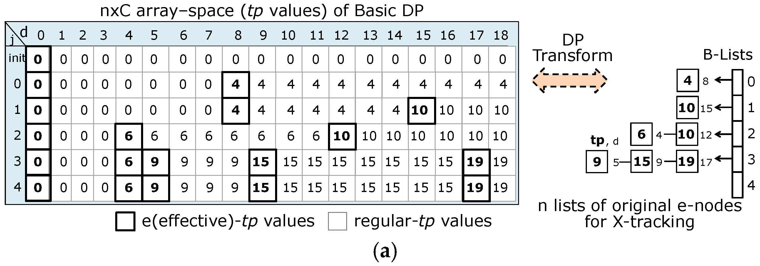
For object j = 0 (w0 = 8, p0 = 4), Step 1 copies the first e-node cn = (tp, d) = (0, 0) of F-list j − 1 to F-list j (since cn.tp < p0 and cn.d < w0). In Step 2 (from head of F-list j − 1), at e-node en = (0, 0), Step 2.1 computes d = en.d + w0 = 8, tp = en.tp + p0 = 4, and decode TP = 0 [(n1.d = 0, n1.tp = 0), (n2.d = C = 18, n2.tp = 0)]. Since d < C and tp = 4 > TP = 0, Step 2.2 adds new e-node = (4, 8) in F-list j = 0 and B-list L0.
For object j = 1 (w1 = 15, p1 = 10), Step 1 copies (0, 0), (4, 8) of F-list j − 1 to F-list j (while cn.tp < p1 and cn.d < w1). In Step 2, at e-node en = (0, 0) of F-list j − 1, compute d = 15, tp = 10, TP = 4 ((n1.d = 8, n1.tp = 4), (n2.d = C = 18, n2.tp = 4)). Since tp = 10 > TP = 4, add new e-node (10, 15) in F-list j = 1 and B-list L1. At en = (4, 8), d = 8 + 15 = 23 > C (no new e-node added).
For object j = 2 (w2 = 4, p2 = 6), Step 1 copies (0, 0) of F-list j − 1 to F-list j. In Step 2, at en = (0, 0) of F-list j − 1, d = 4, tp = 6 > TP = 0, add new e-node (6, 4) in F-list j = 2 and B-list L2. At en = (4, 8) of F-list j − 1, d = 8 + 4 = 12, tp = 4 + 6 = 10 > TP = 4, add new e-node (10, 12). At en = (10, 15), d = 15 + 4 = 19 > C (no new e-node added).
For object j = 3 (w3 = 5, p3 = 9), Step 1 copies (0, 0), (6, 4) of F-list j − 1 to F-list j. In Step 2, at en = (0, 0) of F-list j − 1, d = 5, tp = 9 > TP = 6 (add new e-node (9, 5)). At en = (6, 4) of F-list j − 1, d = 4 + 5 = 9, tp = 6 + 9 = 15 > TP = 6 (add new e-node (15, 9)). At en = (10, 12), d = 17, tp = 19 > TP = 10 (add new e-node (19, 17)).
For object j = 4 (w4 = 12, p4 = 8), Step 1 copies (0, 0), (6, 4) of F-list j − 1 to F-list j. In Step 2, at en = (0, 0) of F-list j − 1, compute d = 12, tp = 8 < TP = 15 (no new e-node added). At en = (6, 4), compute d = 4 + 12 = 16, tp = 6 + 8 = 14 < TP = 15 (no new e-node added). At en = (9, 5), add this remaining (worth) e-node to F-list j and compute d = 5 + 12 = 17, tp = 9 + 8 = 17 < TP = 19 (no new e-node added). At en = (15, 9), add this remaining e-node to F-list j and compute d = 9 + 12 = 21 > C (no new e-node added). At en = (19, 17), add this remaining e-node to F-list j and compute d = 17 + 12 = 29 > C (no new e-node added).
Figure 6 shows another example (n = 15, C = 40), P = {17, 14, 14, 15, 12, 16, 13, 15, 16, 18, 22, 24, 21, 13, 11} and W = {11, 14, 7, 5, 10, 12, 5, 8, 5, 11, 9, 10, 8, 5, 6}. The 223 e-nodes (black + gray) and 103 original e-nodes (black) are reduced over nC = 15 × 40 = 600 cells.

3.2. X-Tracking of the DPT-ListTSR Algorithm

Our X-tracking for solx[n] (Algorithm 8) works on the B-lists (of the original e-nodes), similar to the effective-tps in the 2D array of the basic DP (Algorithm 1: Lines 9–15). On B-list X-tracking, moving left/up (from the B-list Ln−1) is processed by the back pointer in each B-list Lj. Moreover, to simplify the remaining of the X-tracking (after selecting any xj = 1), the B-reduction (Algorithm 8: Line 4) is used to delete some of the original e-nodes of B-lists 0 to j − 1 (if e-node.dnode-j.d) after selecting xj (of node-j(tp, d)).
Algorithm 8: X-tracking (for solx) on B-lists of the DPT-ListTSR algorithm.
  •  start from B-list Ln−1 up to Lj(tp = soltp); tp = Lj.tp; tw = Lj.tw;
  •  while (tp > 0 & j ≥ 0) do
  •   solx = solx∪{j};    // union a select object j (xj = 1) with node-j(tp, d);
  •   call B-reduction (delete e-node(tp, d) of L0 to Lj−1 if e-node.dnode-j.d);
  •   tp = tp-pj; tw = tw-wj; // update remaining (tp, tw);
  •   j = moveLEFT-UP(n, C, j, tp, tw, L); // move to next e-node(tp, d = tw);
  •  end while.
Figure 7a displays an example of X-tracking (n = 5) on B-lists (Figure 5). From list Ln−1, moving starts from n − 1 = 4 with tp = 19 (tw = 17) to select x3 = 1. Next, with tp = 10 (tw = 12) after selecting x2 = 1, B-reduction deletes an unused e-node (tp = 10, d = 15) in list L1 (since e-node.d (= 15) > node-j.d (= 12)) and finally selects x0 = 1. Figure 7b shows a complex example of X-tracking and B-reduction (n = 15) on B-lists (dark color in Figure 6), i.e., after selecting x13 = 1, seven original e-nodes (at j = 0–12, d = 39–40) in B-lists are deleted, after selecting x11 = 1, 14 original e-nodes (at j = 0–10, d = 34–38) in B-lists are deleted, after selecting x10 = 1, 21 original e-nodes (at j = 0–9, d = 24–33) in B-lists are deleted, after selecting x8 = 1, 8 original e-nodes (at j = 0–7, d = 15–23) in B-lists are deleted, etc.

4. 0/1-mKP Solving by Multi-DPT-ListTSR Plus Unbiased Filtering in Efficient Time

To solve the 0/1 mKP, we propose an efficient novel research track (Figure 8a) by starting with the exact DP in exponential time O(m!nC) and ending with polynomial time O(m2n) by our efficient unbiased filtering, while retaining 99% optimal solutions. To solve this complex NP-hard problem (0/1-mKP), we propose three effective algorithms: 1. the multi-DPT-ListTSR algorithm (for m knapsacks) by applying the exact DPT-ListTSR algorithm (in Section 3), 2. the exact-fit (best) knapsack order (with m!-to-m2 reduction by applying the DPT-ListTSR) to achieve the good results as m! orders, and 3. robust unbiased filtering (for polynomial time). Moreover, Figure 8b presents a variety of our parallel reduction models based on medium and coarse grains (pm processors). First, in Section 4.1, we propose the multi-DPT-ListTSR algorithm to find 99% optimal solutions (of the 0/1-mKP) in O(m2[n2, nC]) and hence O(m[n2, nC]) in parallel (p = m processors). Second, in Section 4.2, robust unbiased filtering is incorporated with our multi-DPT-ListTSR in O(m2(n + C′)) or O(m2n) with C′ (<<C) < large n and O(mn) in parallel (p = m processors).

4.1. Efficient Multi-DPT-ListTSR Algorithm for Solving 0/1-mKP

The 0/1-mKP is one of the hardest KPs since it is difficult to find the optimal solutions in O((m + 1)n) by the BnB algorithm, except on small n. For large n, we study the DPT-ListTSR algorithm (in Section 3) first for the 0/1-KP since its optimal solution can be computed in O([n2, nC]) in each knapsack (or the internal effect for the 0/1-mKP (m knapsacks)). Next, we can use m! orders (m knapsacks) directly (for the external effect) in our multi-DPT-ListTSR algorithm for at least 99% optimal solutions in O(m! [n2, nC]) since the more orders there are, the higher the optimal precision. However, that exponential complexity cannot support large m, n, and C. Thus, we propose two efficient order reductions: 1. the top nine (knapsack) orders in O(m[n2, nC]) for the regular datasets and 2. the exact-fit (best) knapsack order in O(m2[n2, nC]) for the irregular datasets.

4.1.1. Top Nine Knapsack Orders for Regular Datasets

Initially, the top nine (knapsack) orders are introduced in our multi-DPT-ListTSR algorithm, which are good enough to solve the 0/1-mKP with 99% optimal solutions for the regular datasets. Each of the top nine orders is obtained by sorting m capacities (Ci, i = 1, 2, 3, …, m). For example (m = 5), the forward order (F) of capacities C = (66, 26, 80, 96, 70) is (1, 2, 3, 4, 5), and the top three orders are increasing (inc) = (2, 1, 5, 3, 4), decreasing (dec) = (4, 3, 5, 1, 2), and combined inc-dec = (2, 4, 1, 3, 5). In this study, the top nine effective orders include increasing (inc), decreasing (dec), combining inc-dec, combining dec-inc, forward (F), backward (B), odd-even (of F), odd-even (of inc), and odd-even (of dec); see a corresponding example in Figure 9. Moreover, each result of the top nine orders can be improved by the Latin square (LS) of m permutations to achieve at least 99% optimal solutions (for the regular datasets). In practice, the partial LS (first nine permutations) of the top nine orders are used to preserve the complexity in O(m[n2, nC]) for m > 9.
Algorithm 9 (multi-DPT-ListTSR) is proposed to solve the 0/1-mKP for each order (of top nine orders/Latin squares of nine orders) in O(m[n2, nC]). Moreover, in some cases, there are different Xs (in X-tracking from many soltws of max soltp), called the nonunique solution Xs, in each knapsack. For the 0/1-KP, X-tracking can start at (soltp, min soltw) or (soltp, max soltw) for different Xs. For the 0/1-mKP (Algorithm 9: Lines 5–6), knapsack i (≤ m − 1) should start at (soltp, max soltw) to allow the better result for the remaining knapsacks, while the last one (i = m) can start at (soltp, min soltw). For example, given a dataset (n = 25, m = 4, C = (20, 30, 40, 50), P = {17, 10, 14, 18, 14, 15, 27, 11, 12, 16, 24, 13, 22, 26, 15, 16, 18, 22, 19, 24, 21, 13, 14, 11, 28}, and W = {11, 4, 14, 3, 7, 5, 4, 4, 10, 12, 6, 5, 7, 6, 8, 5, 11, 9, 5, 10, 8, 5, 3, 6, 8}). In knapsacks K1K2, there are unique X-tracking results, but nonunique X-results occur in knapsack K3 (C3 = 40, n* = 15, j = {0, 2, 4, 5, 8, 9, 11, 14, 15, 16, 17, 19, 20, 21, 23}). Figure 10a shows the result (393) when starting X-tracking at (103, 39), min soltw = 39 in K3. Figure 10b shows the optimal result (398) when starting X-tracking at (103, 40), max soltw = 40 in K3, leading to the better result in knapsack K4 (select j = 0 (w0 = 11, p0 = 17) instead of j = 8 (w8 = 10, p8 = 12) in Figure 10a). Note: In parallel (p = m), we can assign one order per processor for at most m permutation orders (for independent computing for p solutions (at the same time) before selecting the best result).
Algorithm 9: Multi-DPT-ListTSR for one proper order: O(m[n2,nC]).
  • n* = n;
  •  for (i = 1 to m) do
  •   apply DPT-ListTSR (n* objects) on knapsack i (Ki);
  •    call Algorithm 7; // preprocessing (of DPT-ListTSR)
  •    if (i < m) start X-tracking at (max tp, max tw);
  •    else (i = m) start X-tracking at (max tp, min tw);
  •    call Algorithm 8; // X-tracking (of DPT-ListTSR) for max tp
  •    Total profit = Total profit + max tp;
  •   update n* (exclude ki selected objects of knapsack i);
  •  end for i;
  •  return Total profit.

4.1.2. The Exact-Fit (Best) Knapsack Order for Regular and Irregular Datasets

For the irregular datasets, we may use all possible m! orders to find at least 99% optimal solutions in O(m! [n, nC]) but m! orders work on small m only. Thus, for large m, to achieve the optimal precision as m! orders, we propose the exact-fit (best) knapsack order (Algorithm 10) in O(m2[n2, nC]), where both internal and external effects must be solved by the exact DPT-ListTSR algorithm. For the external effect (among m knapsacks), the DPT-ListTSR algorithm is used for computing the exact (TPi, TWi) in each of available knapsacks before selecting Ki with the best exact-fiti = min(dFiti), where different Fiti (dFiti) = CiTWi, ∀im. For instance, Figure 11 shows the exact-fit (best) order for m = 5, C = (66, 26, 80, 96, 70), n = 33, P = {18, 44, 7, 21, 22, 29, 42, 24, 36, 17, 13, 23, 12, 25, 15, 41, 15, 19, 33, 5, 8, 18, 28, 25, 12, 30, 19, 14, 48, 25, 16, 23, 25}, and W = {6, 12, 16, 12, 14, 14, 5, 12, 12, 15, 10, 17, 14, 9, 19, 5, 7, 12, 8, 14, 14, 15, 14, 12, 7, 6, 13, 15, 10, 14, 8, 12, 10}. In Figure 11b, the best order (2, 4, 1, 5, 3) is computed in m(m + 1)/2 = 15 steps by our exact DPT-ListTSR algorithm to achieve the optimal result (726).
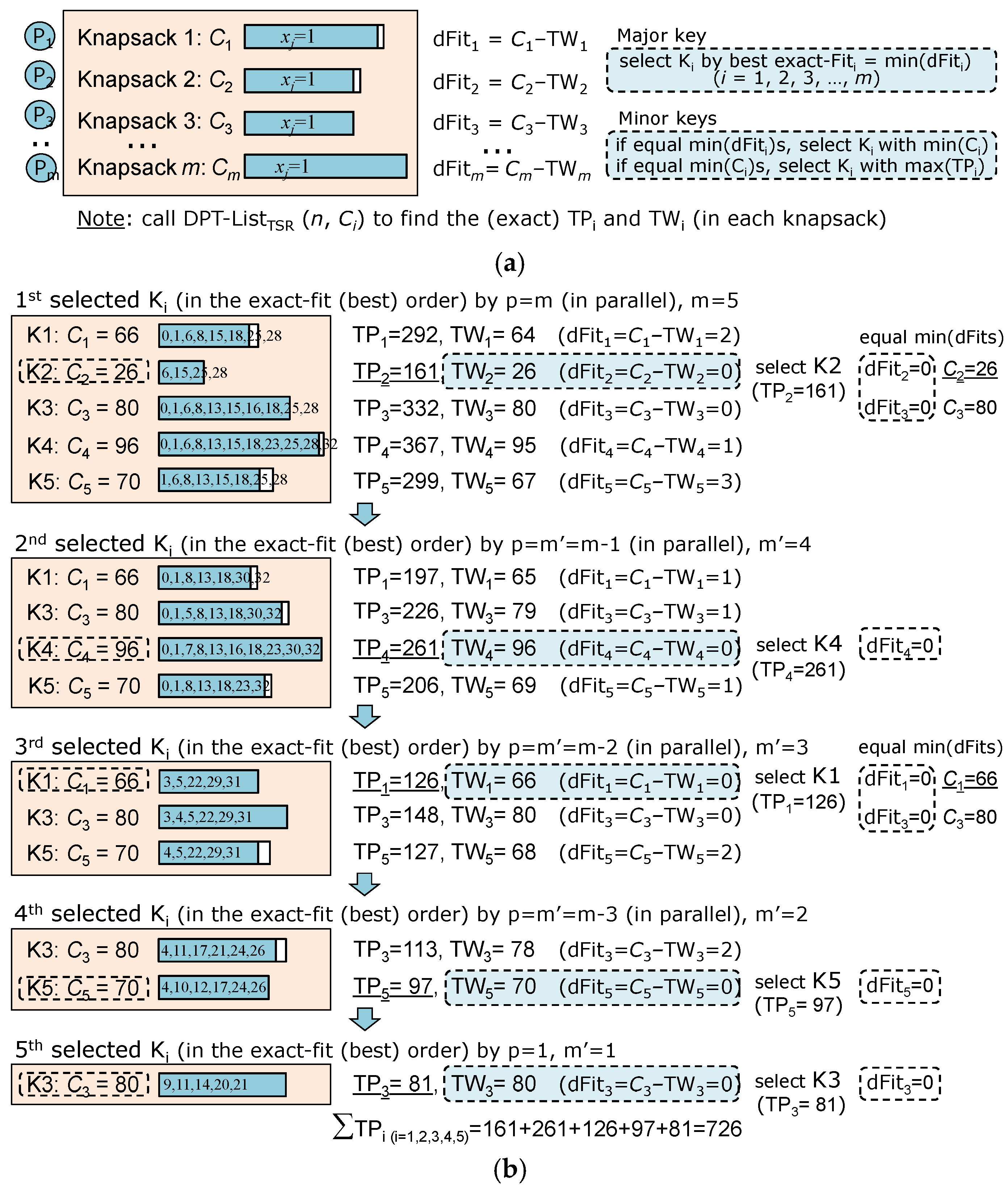
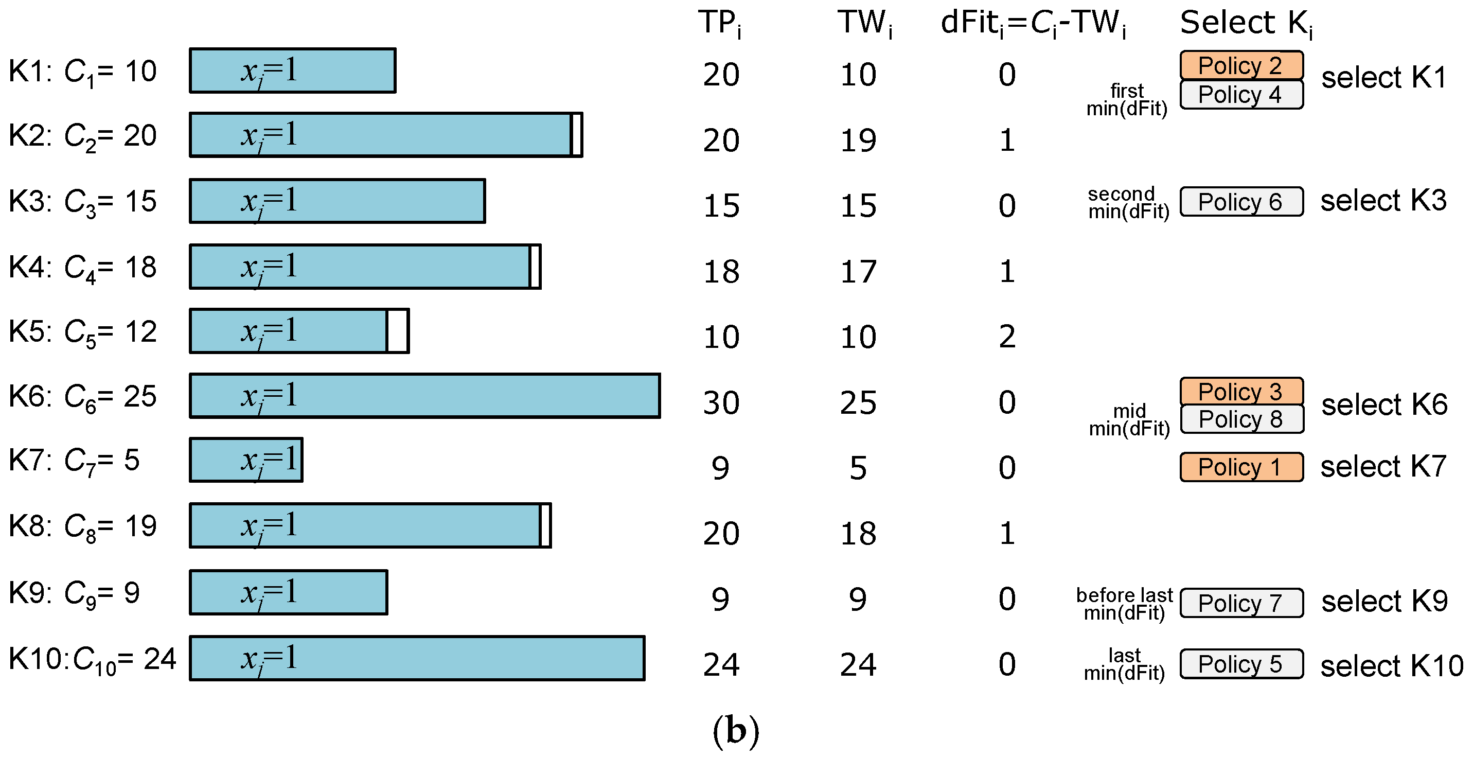
In the first Ki selection, there are m dFiti-results (in m = 5 steps) with two min(dFits) = 0 (in K2, K3) and K2 (min C2) is selected (see conditions in Step 2 of Algorithm 10).
In the second Ki selection, there are 4 dFiti-results and K4 (min(dFit4) = 0) is selected.
In the third Ki selection, there are 3 dFiti-results and K1 (min(dFit1) = 0) is selected.
In the fourth Ki selection, there are 2 dFiti-results and K5 (min(dFit5) = 0) is selected.
In the fifth Ki selection, the last K3 (min(dFit3) = 0) in the last step is selected.
Moreover, for critical decisions in some datasets, there are equal min(dFiti)s in Ki′Ki″. Then, three extra policies (Step 2 in Algorithm 10) are introduced to find the best of the three best results (for the good results as m! orders as much as possible).
Algorithm 10: multi-DPT-ListTSR (the exact-fit (best) knapsack order).
Step 1:
apply DPT-ListTSR for (TPi,TWi) on each of m knapsacks in O(m[n2, nC]) and O([n2, nC]) in parallel (p = m).
Step 2:
select best Ki with min(dFiti); dFiti = Ci -TWi (i = 1, 2, …, m).
In Step 2, for critical min(dFiti), each of the three policies is applied.
   Policy 1: if (there are equal min(dFiti)s), select best Ki with min(Ci);
    if (there are equal min(Ci)s), select best Ki with max(TPi);
  
Policy 2: if (there are equal min(dFiti)s), select best Ki with max(TPi/TWi);
    if (there are equal max(TPi/TWi)s), select best Ki with min(Ci);
    if (there are equal min(Ci)s), select best Ki with max(TPi);
Policy 3: if (there are equal min(dFiti)s), select best Ki with max(TPi);
    if (there are equal max(TPi)s), select best Ki with min(Ci);
Step 3:
update unselected n* = nk and m’ = m − 1.
Step 4:
repeat Step 1–3 on n* and m’ until m’ = 1.
In parallel, the multi-DPT-ListTSR (the exact-fit (best) order) can be processed in O(m[n2, nC]) by p = m. However, O(mnC) in the worst case is not efficient for large m, n, and C. Thus, in Section 4.2, robust unbiased filtering (our key contribution) is presented in efficient O(m2n) by p = 1 and O(mn) by p = m while retaining 99% exact precision.

4.2. Efficient Robust Unbiased Filtering for Polynomial Time Reduction

In our novel research track (Figure 8a), the contribution in polynomial time is achieved by robust unbiased filtering in O(m2(n + C′)) or O(m2n) on C′ (<<C) < large n while retaining 99% optimal solutions. Our (fast and efficient) unbiased filtering can select the outstanding objects (from n objects), and only uncertain objects (n’ < 300) are considered by the DPT-ListTSR algorithm (in each knapsack). For the 0/1-mKP, the parameter (γ, α, β)-setting (in Equations (10)–(14)) was our key contribution to retain 99% optimal precision, as in our previous work (Algorithm 4) [1]. Usually, the critical and uncertain objects (γ, α, and β) could not be easily found. In this study, we performed the experiment on a variety of datasets (including the critical datasets) to classify objects into four groups (see Figure 12) before performing the efficient unbiased filtering. Variables (γ, α) refer to some critical objects (in Groups 1–2), another variable β refers to other critical objects (in Group 4), and most uncertain objects (U) are in Group 3.
n′ = γ + α + U + β < 300
γ = min (10, 0.15 × |Group1|); max γ = 10
α = min (25, 0.85 × |Group2|); max α = 25
β = min (50, 0.70 × |Group4|); max β = 50
U = min (200, |Group3|); max U = 200
From the four groups of object classification (in Figure 12), the dynamic critical region was studied to limit the critical/uncertain objects (n′ < 300) after filtering while retaining 99% optimal precision. For large n, the variable n′ is γ + α + β + U = 10 + 25 + 50 + 200 = 285 since for large C there are a large number of filtering-in objects (xj = 1) and for small C there are a large number of filtering-out objects (xj = 0). Efficient filtering (in Algorithm 11: Line 3) is required (in each Ki) before applying the DPT-ListTSR algorithm to n′ and Ci’. Note: n′ ((temporary) remaining objects after filtering) and n* (remaining objects for next knapsack) are different. For example, Figure 13 shows the result of object classification for filtering (n = 25, m = 2, C = (30, 40), P = {17, 10, 14, 18, 14, 15, 27, 11, 12, 16, 24, 13, 22, 26, 15, 16, 18, 22, 19, 24, 21, 13, 14, 11, 28}, and W = {11, 4, 14, 3, 7, 5, 4, 4, 10, 12, 6, 5, 7, 6, 8, 5, 11, 9, 5, 10, 8, 5, 3, 6, 8}) with four-group classification (P/W-rank in each group). Figure 14 demonstrates the result of filtering-in three objects (6, 13, 3) in knapsack K1 (C = 30) and (temporary) filtering-out four objects (0, 9, 8, 2). For the remaining n′ = 18 and C′ = 17, the DPT-ListTSR selects three objects (22, 10, 24). Then, there are remaining n* = 19, including (0, 9, 8, 2). For knapsack K2 (C = 40), the filtering selects three objects (18, 12, 15), and the DPT-ListTSR selects five objects (5, 7, 11, 21, 1) from n′ = 14, C2 = 18. The result of our multi-DPT-ListTSR + robust filtering is 256 (optimal). In addition, for the irregular datasets, our robust unbiased filtering can select some of n objects before packing the remaining n′ (<300) by the DPT-ListTSR in each knapsack. Figure 15 shows the optimal solution (726) by our efficient filtering, similar to Figure 11 (by our original multi-DPT-ListTSR). See the experimental results of regular and irregular datasets in Section 6.
Algorithm 11: Multi-DPT-ListTSR + robust unbiased filtering.
  • n* = n;
  •  for (i = 1 to m) do
  •   do object classification and unbiased filtering (for Filter-tp) on n*;
  •   apply DPT-ListTSR (n′ < 300) on knapsack i (Ci’);
  •    call Algorithm 7 (preprocessing on remaining n′, Ci’);
  •    if (i < m) start = (max tp,max tw) else start = (max tp,min tw);
  •    call Algorithm 8 (X-tracking on n′ for solx from max tp);
  •    Total profit = Total profit + Filter-tp + max tp;
  •   update n* (exclude ki selected objects of knapsack i);
  •  end for i;
  •  return Total profit.

5. Analysis of Proposed Algorithms

The correctness of the DPT-ListTSR algorithm for solving the 0/1-KP was proven in Section 5.1 and its complexity was analyzed in Section 5.2. For solving the 0/1-mKP, the high (optimal) precision (as m! orders) of the exact-fit (best) knapsack order was presented in Section 5.3. Finally, the 99% optimal precision of the robust unbiased filtering for solving the 0/1-KP and the 0/1-mKP were analyzed in Section 5.4.

5.1. Correctness of the DPT-ListTSR Algorithm

The DPT-ListTSR algorithm (in Section 3) was designed to solve the 0/1-KP in O([n2, nC]) on the efficient lists, which can find the optimal solutions as the best DP (Algorithm 1: O(nC) on a 2D-array (n × C)) before being applied in each of m knapsacks.
Our DPT-ListTSR algorithm can reduce not only the redundant computing time but also the space consumption (of the basic DP: Algorithm 1) while retaining the correctness. Our focus is the DP transformation of the 2D array (nxC) to the efficient lists of e-nodes. Our preprocessing (Algorithm 7) employs two (temporary) F-lists (of objects j − 1 and j) to inherit all worth e-nodes (of objects 0 to j − 1) and compute new e-nodes (improved tp values by the current object j) before saving only the original e-nodes in B-list j.
To clarify our correct transformation, Figure 16 shows the construction of e-nodes (of F-lists j) in Figure 5 (n = 5). For object j = 1 (p1 = 10, w1 = 15), Figure 16a displays the F-list j construction. After the initial copy of two e-nodes (cn = (tp, d) = (0, 0) and (4, 8)) from F-list j − 1 (while cn.tp < p1 and cn.d < w1) to F-list j, the rest of F-list j is fulfilled. For the first e-node en = (0, 0) of F-list j − 1, a new e-node (10, 15) with d = 15 < C and tp = 10 > TP = 4 is added to the end of F-list j. For the next en = (4, 8), compute d = 8 + 15 = 23 > C (no new e-node is added). For object j = 3 (p3 = 9, w3 = 5), Figure 16b shows the F-list j construction in three steps. After the initial copy of two e-nodes (cn = (0, 0) and (6, 4)) from F-list j − 1 (while cn.tp < p3 and cn.d < w3) to F-list j, the rest of F-list j is fulfilled. For en = (0, 0), a new e-node (9, 5) is added to F-list j. Second, for en = (6, 4), a new e-node (6 + 9, 4 + 5) = (15, 9) is added to F-list j. Third, for en = (10, 12), this remaining e-node is not inherited, whereas a new e-node (10 + 9, 12 + 5) = (19, 17) is added to F-list j. Note: Function “inherit remaining e-node” (in Algorithm 7: Line 6) is presented in Figure 16b; see the complex inherited results in Figure 6 (n = 15). Finally, our X-tracking (Algorithm 8) can find solx[n] from the original e-nodes (on the B-lists in Figure 7), similar to the basic DP (on the 2D-array).

5.2. Complexity Analysis of the DPT-ListTSR Algorithm

The time complexity of our DPT-ListTSR algorithm for solving the 0/1-KP is O([n2, nC]), according to the efficient reduction of computing time and using space; see Figure 17 (our efficient time-space reduction). Our time complexity depends on the number of e-nodes of the (temporary) F-list j for all j = 0, 1, 2, 3, …, n − 1, where |F-list j| ≤ 2|F-list j − 1|; see a simple example (n = 5) in Figure 5. The (initial) F-list j contains one e-node (tp, d) = (0, 0). For object j = 0, there are at most two e-nodes (≤2 nodes). For object j = 1 (≤ 4 nodes) and for any j (≤ 2 × 2j−1 nodes), the time complexity of our DPT-ListTSR algorithm can be the best, average, or worst cases, depending on the datasets. Figure 5 displays one of the best cases (n = 5, C = 18, e-nodes = 19, and original e-nodes = 7, reduced from nC = 90 elements). Thus, in this analysis, the best and worst cases can be derived as follows:
-
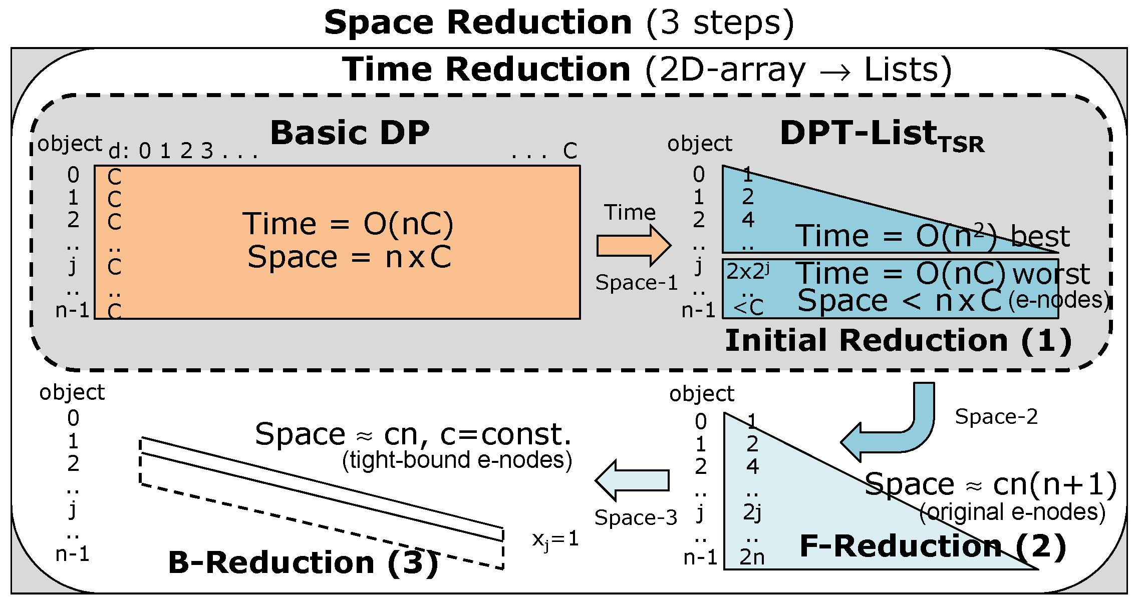
Best case: Total steps (n objects (j = 0 to n − 1)) are approximately 1 + 2 + 4 +…+ 2(j + 1) +…+ 2nn(n + 1) = O(n2).
-
Worst case (rarely occurs): Total steps are approximately 1 + 2 + (≤4) + (≤8) +…+ (≤2 × 2j) +…+ (≈n × C/2) = O(nC).
The worst case (the e-nodes of F-listn−1 = |F-listn−1| ≈ C) hardly occurs due to some remaining e-nodes of F-list j − 1 are not inherited to F-list j (see a clarified example in Figure 16b) and no additional new e-nodes in F-list j when considering some (worst) objects j (such as large wj or tiny profit pj) by two conditions: 1. node.tp + pj < tp[d] (no improved tp) and 2. node.d + wj > C (at d + wj, object j cannot be packed in the knapsack), such as no additional new e-node for object j = 4 (in Figure 5). Figure 6 shows an example of a regular/average case (n = 15, C = 40, nC = 600, e-nodes = 223, and original e-nodes = 103). The time complexity of the average case arises in most datasets (≈(best + worst)/2 < nC/2). Since a weight wj of object j can be 1 ≤ wj < C, the average wj is approximately C/n. For wjC/n, usually no e-node is added (because of the condition node.d + wj > C).
For m knapsacks, the time complexity of our multi-DPT-listTSR algorithm for solving the 0/1-mKP is O(m[n2, nC]) with any effective knapsack order (including top nine orders) and O(m2[n2, nC]) for the exact-fit (best) order in m(m + 1)/2 steps; see Section 5.3.
For space complexity, Figure 17 illustrates our three steps of space reduction: 1. e-nodes (<nC), 2. original e-nodes, and 3. tight bound of e-nodes; see Figure 5 (n = 5, C = 18) and Figure 7b (n = 15, C = 40). In our experiment, Section 6.1, displays the observed results (n ≤ 3000), where after F-reduction the original e-nodes are a function of cn2 (<n3, c = a constant) and hence after B-reduction the original e-nodes are less than n2.

5.3. High (Optimal) Precision (as m! Orders) of the Exact-Fit (Best) Knapsack Order

In our novel research track (Figure 8), we study by starting with the exact DP for the optimal solution in one knapsack to m knapsacks. In Section 3, we propose the DPT-ListTSR algorithm to find the optimal solution in O([n2, nC]) for each knapsack. In Section 4, we propose the efficient order reduction for m knapsacks (over m! orders), which are 1. the top nine effective orders in our multi-DPT-ListTSR algorithm in O(m[n2, nC]) for the regular datasets, and 2. the exact-fit (best) order in our multi-DPT-ListTSR algorithm in O(m2[n2, nC]) for the irregular datasets, where the DPT-ListTSR algorithm is applied in the internal and external effects (in each knapsack and among m knapsacks).
For the regular datasets, an effective order is increasing Ci; see Figure 18 (selecting k candidates (objects), 0 ≤ jn − 1, for m positions (knapsacks with capacity Ci, i = 1, 2, …, m) in a company/organization, the profit pj (knowledge), and the weight wj (negative attitude/greedy weight)). For large m, the (fast) top nine effective orders (in Section 4.1.1) are presented and later improved by the LS of m permutations, where the partial LS (first nine permutations of each order) is concerned in O(m[n2, nC]), see Table 1 (the proposed reduction orders and all possible m! orders (for 5 ≤ m ≤ 100)).
For the irregular datasets, we can use m! orders to achieve at least 99% optimal solutions but in exponential time O(m! [n2, nC]). To reduce the time complexity and retain 99% optimal precision, the exact DPT-ListTSR algorithm is applied for not only the internal effect (for the optimal solution in each knapsack) but also the external effect (for the best order among m knapsacks). For the external effect, the DPT-ListTSR algorithm is used to find all exact-fit knapsacks before selecting the best knapsack and repeating the same process for the remaining objects and knapsacks. The exact-fit (best) order (Algorithm 10) is determined in m(m + 1)/2 steps in O(m2[n2, nC]). In particular, the best knapsack Ki is selected by the best exact-fiti = min(dFiti); dFiti = CiTWi, where the exact TPi and TWi are computed by the DPT-ListTSR algorithm in each of the available knapsacks; see Figure 11 (n = 33, m = 5). Moreover, if there are equal min(dFiti)s in more than one Ki (in the critical decision) in step 2 of Algorithm 10, then three proper policies are used to find the best of three best solutions. See the confirmed results (99% optimal solutions) in Section 6.3.

5.4. High (Optimal) Precision of the Robust Unbiased Filtering

The exact DP + unbiased filtering [1] can solve the 0/1-KP in O(n + C′), C′ << C with at least 95% optimal precision. Thus, we can adopt the process of unbiased filtering for the 0/1-mKP. Initially, all objects are classified (into four groups) by dynamic weighting (dw), integrated from three effective ranks (P/W, P, W); see Figure 19a, where two parameters (α, β)) were defined to handle special objects (called outliers) in unbiased filtering [1] for the 0/1-KP with 95% optimal solutions. In this study, to achieve 99% optimal solutions for the 0/1-mKP, the (γ, α, β) parameters are introduced by studying all datasets (i.e., most datasets are regular (≈90%) and irregular datasets are ≈10%). In our robust unbiased filtering, the (γ, α, β, U) parameters are determined in Equations (10)–(14), where the critical objects are in low rank in Group 1 (γ) and Group 2 (α) and in top rank in Group 4 (β), and most uncertain objects (U) are in Group 3. Figure 19a shows that some objects (around the critical points in the three ranks (P/W, P, or W)) are the critical objects (γ, α, β). All uncertain/critical objects (n′< 300) can be solved by the DPT-ListTSR algorithm in O(n + C′). Figure 19b shows the idea of 99% optimal precision (due to our robust unbiased filtering) in each knapsack of the 0/1-mKP; see in the observed results (in Section 6).

6. Experimental Results

Experiments were conducted to evaluate the DPT-ListTSR algorithm and robust unbiased filtering for the 0/1-KP (Section 6.1) to ensure at least 99% optimal precision (in each knapsack) before applying to the 0/1-mKP (Section 6.2 and Section 6.3) by the multi-DPT-ListTSR algorithm (the best knapsack-order for m knapsacks) and robust unbiased filtering.

6.1. Results of the DPT-ListTSR (One Knapsack) and Robust Unbiased Filtering

For solving the 0/1-KP, we generated a variety of random datasets (dynamic seeds) with a number of uniform distributions to obtain the profits and weights of n objects (n ≤ 10,000). The experiment was conducted to evaluate the performance of robust unbiased filtering. In the experimental results, our DPT-ListTSR + robust unbiased filtering could find the exact solutions in each of the datasets (n ≤ 10,000), while there were 223 (of 10,000) datasets for which the recent TSReduction + unbiased filtering [1] could not find the optimal solutions. Table 2 shows the empirical results of the first 23 of 223 special datasets (or irregular datasets), n = 12, 14, 21, 26, 39, …, 385 (observed on n = 5, 6, 7, …, 9999, 10,000).
Table 3 presents the optimal performance of our DPT-ListTSR + robust unbiased filtering for at least 99% optimal solutions (on n ≤ 10,000) compared to our previous work [1]. In this experiment, there exist irregular datasets ≈10% (from all 10,000 random datasets), where unbiased filtering (in TSReduction) [1] could handle ≈5% and our robust unbiased filtering (in DPT-ListTSR) could handle ≈9.9%. Table 4 displays our space reduction, observed on n ≤ 3000 (with runtime < 1 min per n). Our F-reduction can save space 69–92%, and our B-reduction can save space 84–93%.

6.2. Results of the Multi-DPT-ListTSR (m Knapsacks) and Robust Unbiased Filtering

For solving the 0/1-mKP, the optimal performance of our multi-DPT-ListTSR algorithm with the proper (knapsack) orders (i.e., top nine orders, Latin squares, the exact-fit (best) order) was evaluated by comparison to the optimal solutions. In practice, the fast response time of our multi-DPT-ListTSR with robust unbiased filtering was observed, while retaining the high performance. In this experiment, a number of random datasets were generated for n (≤10,000) objects and m (≤100) knapsacks with a variation of capacities (i.e., Ci ± 10, Ci ± 15, Ci ± 20, etc.). In addition, the benchmark datasets [34] were observed and the empirical results were compared to the optimal solutions.
In performance (total profit) evaluation, we focus on the investigation of 1. the exact-fit best (knapsack) order in our multi-DPT-List algorithm (for 99% optimal solutions in theory) and 2. the robust unbiased filtering (in polynomial time) to confirm 99% optimal solutions. We implemented our multi-DPT-List (the exact-fit best order) and the fast multi-DPT-List + robust filtering compared to the optimal solutions. For the practical polynomial-time evaluation, the fast response time of our multi-DPT-List + robust filtering was compared to the quick multi-GH+ (a well-known heuristic algorithm).
For the performance comparison, the (known) optimal solutions of the 0/1-mKP (in Column 2 of Table 5, Table 6, Table 7, Table 8, Table 9 and Table 10) can be computed by using a large knapsack (Cs = i = 1   m C i ) by the exact DP or our DPT-List in the (regular and irregular) datasets.
The implemented programs of three main approaches (in this experiment) are
Exact1.1 Multi-DPT-List (exact-fit best order) O(m2[n2,nC])
Exact + Filtering2.1 Fast multi-DPT-List + filtering (exact-fit best order)
2.2 Fast multi-DPT-List + filtering (top 9 orders + partial LSs)
2.3 Fast multi-DPT-List + filtering (top 9 orders)
O(m2n)
O(mn)
O(mn)
Heuristic3.1 Quick multi-GH (P/W rank) (top 9 orders)
3.2 Improved multi-GH+ (P/W rank) (top 9 orders)
3.3 Improved multi-GH+ (P/W rank) (top 9 + full LS orders)
O(mn)
O(mn)
O(m2n)
First, we evaluated the performance of our mDPT-List and fast mDPT-List + filtering with m! orders (for small m = 2, 3, 4), compared to the optimal solutions. For m ≤ 4, our approach can find the optimal solutions in most datasets; see Columns 3 and 4 in Table 5, Table 6 and Table 7. For m > 4, we investigated the effect of robust filtering plus the top nine effective orders and partial Latin squares (Columns 4 and 5 in Table 8 and Table 9). For the regular datasets (n ≤ 10,000, m ≤ 100), our mDPT-List + filtering (top nine orders) yielded 99% optimal solutions.
Second, we aimed to compare among the fast polynomial-time algorithms (O(mn) − O(m2n)) by observing the effect of the top nine effective orders; see Columns 4–7 in Table 8 and Table 9. For m ≤ 100 and n ≤ 10,000, the results (total profits) of our mDPT-List + filtering (in Column 5) were compared to those of the quick mGH+ (P/W rank) in Columns 6–7 (response time < 1 s). For the regular datasets, our fast mDPT-List + filtering (in Column 5) yielded most optimal solutions, while the results of the quick mGH+ (in Column 6) and its improvement with LS of 9 m orders (in Column 7) were far from the optimal solutions, especially when using many knapsacks (m > 10). Note: GH (P/W rank) is frequently used in many meta-heuristic algorithms (i.e., GA, swarm, etc.) for the good initial solutions to solve the 0/1-KP and GH+ is used in unbiased filtering [1] (p. 199) and in robust unbiased filtering (in this study). In the comparison, we use the improved mGH+ with the Latin squares of top nine orders (for 9 m orders/iterations to emulate the evolution process of GA/swarm optimization). For most datasets, the mGH+ (9m orders) could not find the optimal solutions in each knapsack since it included uncertain object(s) in the solution. However, it is not the problem in our robust unbiased filtering since all uncertain objects (n′ < 300) were considered by the exact DPT-List with 99% optimal precision.
In our initial observation and analysis, for m = 2 (n ≤ 10,000), the mDPT-List + filtering (m! orders) in Table 5 yielded 100% optimal solutions. For m = 3, 4 (n ≤ 10,000), our approach (m! orders) in Table 6 and Table 7 yielded 99.9% optimal solutions. Next, we found that (for the irregular datasets) the top nine orders were not sufficient to find the optimal solutions ≥99%, especially m ≥ 5. Then, we investigated the effect of the LS of the top nine orders (see Column 4 in Table 8, Table 9 and Table 10). Moreover, Table 10 and Table 11 report the irregular datasets found during the execution of each dataset (n ≤ 10,000), where any dataset is called “irregular” when the top nine orders could not find the optimal solution. For m ≥ 5, we performed an intensive study and experiment to observe each of n ≤ 10,000 (m ≤ 100) and found that a number of irregular datasets increased when m increased (see Column 6 in Table 11). Hence, the exact-fit (best) knapsack order is applied to solve this problem.
After performing the intensive study and comparison (on large n ≤ 10,000), we found that for the irregular datasets, our mDPT-List + robust unbiased filtering (the exact-fit (best) order in O(m2n)) could find at least 99% optimal solutions as those of the original mDPT-List (O(m2[n2,nC])); see a report of observed frequency of nonoptimal solutions (0%) of our approach in Table 11 (Column 4).
Finally, we performed an extra experiment to evaluate the performance of our mDPT-List on the benchmark datasets [34] available at http://or.dei.unibo.it/library (accessed on 13 June 2020). Table 12 and Table 13 show the empirical results of our mDPT-List (the best knapsack order in O(m2[n2, nC])) and our fast mDPT-List + robust filtering (the best knapsack order in O(m2n)), compared to the regular mDP (O(m2nC)) and the optimal solutions.
For (n:m = 100:10) 10 datasets [34], the results (in Table 12) showed that our mDPT-List (without/with filtering (the best order, LS orders, top nine orders)) could find the optimal solutions (Columns 4–7), while the results (Column 8) of the quick mGH+ (9 m orders in 9 m iterations) were not optimal.
For (n:m = 200:20, 300:30, 500:50) 20 datasets [34], most optimal solutions of these critical datasets were unknown (see Table 13) since the DP-packing in one large knapsack (Cs = i = 1   m C i ) may be overpacking. Figure 20a shows an example of overpacking, when some objects in the critical datasets (such as some valuable objects j (high pj/wj) but large wj) cannot be packed in any knapsack i with capacity Ci, except in the extra space of one knapsack of large capacity Cs. In these critical datasets, our mDPT-List with the best order (in Columns 5 and 6) yielded good results, which were close to or equal to the optimal solutions and outperformed those of LSs (9m) of top nine orders (in Columns 7–8).
In our contribution, we focus on large n. The fast mDPT-List + filtering (top nine orders) in O(mn) is good for the regular datasets with 99% optimal solutions (Table 5, Table 6, Table 7, Table 8, Table 9 and Table 12). For the irregular datasets (Table 11), our fast mDPT-List (the best order) + filtering in O(m2n) can find 99% optimal solutions similar to our original mDPT-List (the best order). Thus, for the regular and irregular datasets, our fast mDPT-List + filtering (the best order) is sufficient to achieve 99% optimal solutions in polynomial time O(m2n). Moreover, for the critical/special benchmark datasets, we have intensively studied by the experiment (in Section 6.3) to improve the solutions (Column 4 in Table 13).

6.3. Extra Experiment and Additional Improvement on Critical Datasets

To improve the results of the critical datasets (benchmark datasets [34]), we have to find all possible critical decisions, such as 1. nonunique Xs (in X-tracking (see an example in Figure 10) in Section 4.1.1) and 2. equal min(dFits) in more than one knapsacks (in the exact-fit (best) order (see an example in Figure 11) in Section 4.1.2) and provide the right policies to handle them. Clearly, if there is only one min(dFiti), dFiti = CiTWi, we can select the best knapsack Ki directly for the best order. By the DP-packing, there may be many equal min(dFiti)s in Ki′Ki″ but only one Ki is selected (at a time), and this decision may cause the local optimal problem. To handle this problem, the top three effective policies are introduced in Algorithm 10, and the best of three best results is our final solution. However, to achieve the better results of these critical/special datasets, we add the other effective policies 4–8 in Algorithm 10 (step 2) to cover the other critical decisions; see an example in Figure 20b, i.e., select Ki with min(dFiti) at the first, last, second, before last, and mid policies (in policies 4–8). Figure 20b shows the detail of selecting the best Ki (m = 10 knapsacks, Ci = (10, 20, 15, 18, 12, 25, 5, 19, 9, 24)) with eight critical decisions (i.e., assume there are six min(dFiti)s = 0 in Ki, i = 1, 3, 6, 7, 9, 10) for selecting the best Ki (in the best order) with one policy for one result (solTP). In this experiment, the improved results (max (solTPi=1–8)) in Column 4 (Table 13) were stable under these eight policies. In each critical dataset, the results (Column 4) were improved due to the exact DPT-List packing plus the proper critical handling (by our eight policies for the best knapsack order).
In the regular comparison of our mDPT-List + robust unbiased filtering (the best knapsack order) on 20 critical datasets (in Table 13), our robust unbiased filtering (using top three policies) yielded (9 of 20) best results (Column 6), which outperformed the results (Column 7) of using LSs of top nine orders (9 m). In the superior improvement of our eight effective policies (in the extra experiment), the extra mDPT-List yielded (16 of 20) best results (Column 4), while the other 4 of 20 best results (Column 3) were fulfilled by robust filtering due to the (unbiased) preselecting and the less problem of nonunique Xs in the X-tracking by DPT-List (on small n′ < 300) in each knapsack. Obviously, for the unique X, our mDPT-List (with/without filtering) yields the same result.
In addition, the response times of three mDP algorithms (basic mDP, mDPT-List, and mDPT-List + filtering) were compared in this experiment (under the same 99% optimal precision). In theory, three different time complexities of these mDP algorithms are 1. O(m!nC) in the basic mDP (m! orders), 2. O(m2[n2, nC]) in the mDPT-List (the best order), and 3. O(m2n) in the fast mDPT-List + filtering (the best order). Due to our efficient unbiased filtering, the response time of our fast mDPT-List + filtering for n = 20,000 and m = 20 was less than one second, that of the best mDPT-List for n = 20,000 was 10 min, that of the basic mDP for n = 20,000 was more than one hour and so on for other large n.
Next to simplify the comparison and discussion (for the 0/1-mKP solving with the critical datasets), we employ the triple-right rule (right man, right place, and right time). Figure 21 displays the improvement of our multi-DPT-ListTSR algorithm (our novel research track in Figure 8) to reach 99% optimal solutions in efficient time.
In theory, the exact BnB algorithm can find the exact solution of the 0/1-mKP but in O((m + 1)n) with the right man and right place but not the right time. In practice, the multi-GH+ (with 9 m LS-orders) can find the good solutions in polynomial time but those solutions may not be optimal because it only confirms the right time rule. In this study (Figure 21), we study and apply the exact DPT (in theory) and the efficient unbiased filtering (in practice) to achieve triple-right packing (right man (object), right place (knapsack), and right time (O(m2n))). Our contribution is the m!-to-m2 reduction; see the highlight space of our improvement in Figure 21. This tight-bound reduction starts with the exact DPT for one knapsack (selecting the right object), uses the exact-fit (best) order for m knapsacks (putting the right object in the right knapsack), and ends with robust unbiased filtering (putting the right object in the right knapsack at the right time).
The comparison of our multi-DPT-List + robust filtering and the recent HyMKP [34] is demonstrated in Table 14. In practice (with large n (≤10,000 in this experiment)), our multi-DPT-List + robust filtering yielded 99% optimal results in O(m2n); see results in Table 5, Table 6, Table 7, Table 8, Table 9, Table 10, Table 11 and Table 12, while the results of quick multi-GH+ in O(m2n) were not optimal. For the HyMKP study [34], there is no available result for n > 500 since for large n the partial BnB (MULKNAP program) in the HyMKP (Algorithm 5) may not find the optimal solution in τ secs. Then, the reflect multi-graph MKP (with increasing n-weights (wj) in Algorithm 6 (O(mnC)) can provide the comparable results to our multi-DPT-List (with top nine orders) in the regular datasets, according to the looping on weights and C, similar to the DP (Algorithm 1) for each of m knapsacks. For the irregular datasets, v-rounds of decompositions of HyMKP are used to improve the initial solution. However, (for large n) the process of Algorithm 6 may take a long time to reach the 99% optimal solutions due to its complexity O(mnC), while our exact-fit best (knapsack) order of multi-DPT-List + efficient filtering in O(m2n) can find 99% optimal solutions as m! orders.
For n ≤ 500 (in the critical datasets), the HyMKP model yielded 99.9% optimal solutions by the partial BnB (MULKNAP) program in τ secs. Thus, for n ≤ 500 we can adopt that MULKNAP program in our approach for achieving 99.9% optimal solutions.
Finally, after achieving the good performance (99% optimal solutions) of our multi-DPT-ListTSR + robust filtering in the efficient time O(m2n), we can improve the time complexity to O(mn) in parallel (by using p = m processors).
Moreover, to handle the critical datasets in parallel, we can achieve the global best result in parallel (by p = m processors), such as Column 3 (in Table 13), by combining the local best result of the parallel multi-DPT-ListTSR in O(m[n2, nC])) in Column 4 and the local best result of the parallel multi-DPT-ListTSR + robust filtering in O(mn) in Column 6 for the best of the best results (in Column 3) in O(m[n2, nC])), which is efficient, especially in average ≈ O(mn3) if C = max(Ci) ≤ n2.
In practical 0/1-mKP applications (for large n), if the fast computing time is the most important factor (in the regular and irregular datasets), our multi-DPT-List + robust filtering in O(m2n) or O(mn) in parallel (p = m) with 99% optimal solutions is good enough. However, if the high optimal performance is the most important factor (in the critical datasets and in the critical 0/1-mKP applications), the integration (of the original multi-DPT-ListTSR and the fast multi-DPT-ListTSR + robust filtering) provides higher precision (i.e., 99.9% optimal solutions) in efficient O(m[n2, nC]) in parallel (p = m) or O(mn2) in the best case and O(mn3) in average if Cn2.

7. Conclusions

In this study, to solve the complex 0/1-mKP (m knapsacks) in polynomial time we introduced a novel research track with hybrid integration of DP transformation (for the optimal solution in each knapsack) and robust unbiased filtering (for polynomial time). First, the efficient DPT-ListTSR algorithm was proposed to find the optimal solutions of the 0/1-KP in O([n2, nC]) over O(nC) before being applied in the 0/1-mKP. Second, for solving the 0/1-mKP we proposed the multi-DPT-ListTSR with the exact-fit (best) knapsack order (m!-to-m2 reduction) with 99% optimal solutions in O(m2[n2, nC]) over O(m![n2, nC]). Third (for large n, massive C), robust unbiased filtering was incorporated into our multi-DPT-ListTSR to solve the 0/1-mKP in efficient O(m2n) over O(mnC) of the recent HyMKP, while retaining 99% optimal solutions. The experiment was conducted to evaluate the performance of our multi-DPT-List + robust unbiased filtering (with 99% optimal solutions) on random and benchmark datasets (n ≤ 10,000, m ≤ 100). Practically (for large m, n, and C), our multi-DPT-ListTSR + robust unbiased filtering (O(m2n)) could find 99% optimal solutions (as the original multi-DPT-ListTSR (O(m2[n2, nC])) in polynomial time.
In our current research, we apply our multi-DPT-ListTSR + robust unbiased filtering to solve the multi-container packing. In the future study, we will modify our unbiased filtering idea to solve another popular NP-hard problem (i.e., traveling salesman and logistic transportation, etc.) in efficient time with expected high optimal performance.

Author Contributions

Conceptualization, P.B. and J.W.; methodology, P.B.; software, P.B.; validation, P.B. and J.W.; formal analysis, J.W.; investigation, P.B.; writing—original draft preparation, P.B.; writing—review and editing, J.W.; visualization, P.B.; supervision, J.W. All authors have read and agreed to the published version of the manuscript.

Funding

This research was funded by the School of Science, King Mongkut’s Institute of Technology Ladkrabang (KMITL), Bangkok, Thailand, grant number [CW-011-2/2562].

Institutional Review Board Statement

Not applicable.

Informed Consent Statement

Not applicable.

Data Availability Statement

Not applicable.

Acknowledgments

The authors would like to deeply thank the School of Science, King Mongkut’s Institute of Technology Ladkrabang (KMITL), Bangkok, Thailand for the Ph.D. research grant (CW-011-2/2562) to Patcharin Buayen. In addition, they would like to gratefully thank Phra-phrom Kunaporn (P.A. Pa-yut-tao) with his “Put-ta-tum” Buddhism-handbook for fulfilling their exact understanding and good decision-making. Last, they would like to gloriously honor their beloved King Bhumibol Adulyadej for the great inspiration in the optimistic study through positive thinking plus critical rethinking.

Conflicts of Interest

The authors declare no conflict of interest. The funders had no role in the design of the study; in the collection, analyses, or interpretation of data; in the writing of the manuscript; or in the decision to publish the results.

References

  1. Buayen, P.; Werapun, J. Parallel time-space reduction by unbiased filtering for solving the 0/1-knapsack problem. J. Parallel Distrib. Comput. 2018, 122, 195–208. [Google Scholar] [CrossRef]
  2. Aisopos, F.; Tserpes, K.; Varvarigou, T. Resource management in software as a service using the knapsack problem model. Int. J. Prod. Econ. 2013, 141, 465–477. [Google Scholar] [CrossRef]
  3. Vanderster, D.C.; Dimopoulos, N.J.; Parra-Hernandez, R.; Sobie, R.J. Resource allocation on computational grids using a utility model and the knapsack problem. Future Gener. Comput. Syst. 2009, 25, 35–50. [Google Scholar] [CrossRef]
  4. Bas, E. A capital budgeting problem for preventing workplace mobbing by using analytic hierarchy process and fuzzy 0-1 bidimensional knapsack model. Expert Syst. Appl. 2011, 38, 12415–12422. [Google Scholar] [CrossRef]
  5. Camargo, V.C.B.; Mattiolli, L.; Toledo, F.M.B. A knapsack problem as a tool to solve the production planning problem in small foundries. Comput. Oper. Res. 2012, 39, 86–92. [Google Scholar] [CrossRef]
  6. Fukunaga, A.S.; Korf, R.E. Bin completion algorithms for multicontainer packing, knapsack, and covering problems. J. Artif. Intell. Res. 2007, 28, 393–429. [Google Scholar] [CrossRef]
  7. Rooderkerk, R.P.; van Herrde, H.J. Robust optimization of the 0-1 knapsack problem: Balancing risk and return in assortment optimization. Eur. J. Oper. Res. 2016, 250, 842–854. [Google Scholar] [CrossRef]
  8. Ahmad, S.J.; Reddy, V.S.K.; Damodaram, A.; Krishna, P.R. Delay optimization using Knapsack algorithm for multimedia traffic over MANETs. Expert Syst. Appl. 2015, 42, 6819–6827. [Google Scholar] [CrossRef]
  9. Wang, E.; Yang, Y.; Wu, J. A Knapsack-based buffer management strategy for delay-tolerant networks. J. Parallel Distrib. Comput. 2015, 86, 1–15. [Google Scholar] [CrossRef]
  10. Wedashwara, W.; Mabu, S.; Obayashi, M.; Kuremoto, T. Combination of genetic network programming and knapsack problem to support record clustering on distributed databases. Expert Syst. Appl. 2016, 46, 15–23. [Google Scholar] [CrossRef]
  11. Kellerer, H.; Pferschy, U.; Pisinger, D. Dynamic Programming. In Knapsack Problem; Springer: Berlin, Germany; New York, NY, USA, 2004; pp. 20–26. [Google Scholar]
  12. Monaci, M.; Pferschy, U.; Serafini, P. Exact solution of the robust knapsack problem. Comput. Oper. Res. 2013, 40, 2625–2631. [Google Scholar] [CrossRef] [PubMed]
  13. Rong, A.; Figueira, J.R.; Klamroth, K. Dynamic programming based algorithms for the discounted {0-1} knapsack problem. Appl. Math. Comput. 2012, 218, 6921–6933. [Google Scholar] [CrossRef]
  14. Rong, A.; Figueira, J.R.; Pato, M.V. A two state reduction based dynamic programming algorithm for the bi-objective 0-1 knapsack problem. Comput. Math. Appl. 2011, 62, 2913–2930. [Google Scholar] [CrossRef]
  15. Rong, A.; Figueira, J.R. Dynamic programming algorithms for the bi-objective integer knapsack problem. Eur. J. Oper. Res. 2014, 236, 85–99. [Google Scholar] [CrossRef]
  16. Cunha, A.S.; Bahiense, L.; Lucena, A.; Souza, C.C. A new lagrangian based branch and bound algorithm for the 0-1 knapsack problem. Electron. Notes Discret. Math. 2010, 36, 623–630. [Google Scholar] [CrossRef]
  17. Li, X.; Liu, T. On exponential time lower bound of knapsack under backtracking. Theor. Comput. Sci. 2010, 411, 1883–1888. [Google Scholar] [CrossRef]
  18. Calvin, J.M.; Leung, J.Y.-T. Average-case analysis of a greedy algorithm for the 0/1 knapsack problem. Oper. Res. Lett. 2003, 31, 202–210. [Google Scholar] [CrossRef]
  19. Truong, T.K.; Li, K.; Xu, Y. Chemical reaction optimization with greedy strategy for the 0-1 knapsack problem. Appl. Soft Comput. 2013, 13, 1774–1780. [Google Scholar] [CrossRef]
  20. Balas, E.; Zemel, E. An algorithm for large zero-one knapsack problems. Oper. Res. 1980, 28, 1130–1154. [Google Scholar] [CrossRef]
  21. Guastaroba, G.; Savelsbergh, M.; Speranza, M.G. Adaptive kernal search: A heuristic for solving mixed integer linear programs. Eur. J. Oper. Res. 2017, 263, 789–804. [Google Scholar] [CrossRef]
  22. Lim, T.Y.; Al-Betar, M.A.; Khader, A.T. Taming the 0/1 knapsack problem with monogamous pairs genetic algorithm. Expert Syst. Appl. 2016, 54, 241–250. [Google Scholar] [CrossRef]
  23. Sachdeva, C.; Goel, S. An improved approach for solving 0/1 knapsack problem in polynomial time using genetic algorithms. In Proceedings of the IEEE International Conference on Recent Advances and Innovations in Engineering, Jaipur, India, 9–11 May 2014. [Google Scholar]
  24. Bansal, J.C.; Deep, K. A modified binary particle swarm optimization for knapsack problems. Appl. Math. Comput. 2012, 218, 11042–11061. [Google Scholar] [CrossRef]
  25. Bhattacharjee, K.K.; Sarmah, S.P. Shuffled frog leaping algorithm and its application to 0/1 knapsack problem. Appl. Soft Comput. 2014, 19, 252–263. [Google Scholar] [CrossRef]
  26. Moosavian, N. Soccer league competition algorithm for solving knapsack problem. Swarm Evol. Comput. 2015, 20, 14–22. [Google Scholar] [CrossRef]
  27. Zhang, J. Comparative study of several intelligent algorithms for knapsack problem. Procedia Environ. Sci. 2011, 11, 163–168. [Google Scholar] [CrossRef]
  28. Zou, D.; Gao, L.; Li, S.; Wu, J. Solving 0-1 knapsack problem by novel global harmony search algorithm. Appl. Soft Comput. 2011, 11, 1556–1564. [Google Scholar] [CrossRef]
  29. Lv, J.; Wang, X.; Huang, M.; Cheng, H.; Li, F. Solving 0-1 knapsack problem by greedy degree and expectation efficiency. Appl. Soft Comput. 2016, 41, 94–103. [Google Scholar] [CrossRef]
  30. Pavithr, R.S. Gursaran, Quantum inspired social evolution (QSE) algorithm for 0-1 knapsack problem. Swarm Evol. Comput. 2016, 29, 33–46. [Google Scholar] [CrossRef]
  31. Zhao, J.; Huang, T.; Pang, F.; Liu, Y. Genetic algorithm based on greedy strategy in the 0-1 knapsack problem. In Proceedings of the 2009 Third International Conference on Genetic and Evolutionary Computing, Guilin, China, 14–17 October 2009. [Google Scholar]
  32. Zhou, Y.; Chen, X.; Zhou, G. An improved monkey algorithm for 0-1 knapsack problem. Appl. Soft Comput. 2016, 38, 817–830. [Google Scholar] [CrossRef]
  33. Sanchez-Diaz, X.; Ortiz-Bayliss, J.C.; Amaya, I.; Cruz-Duarte, J.M.; Conant-Pablos, S.E.; Terashima-Marin, H. A feature-independent hyper-heuristic approach for solving the knapsack problem. Appl. Sci. 2021, 11, 10209. [Google Scholar] [CrossRef]
  34. Dell’Amico, M.; Delorme, M.; Iori, M.; Martello, S. Mathematical models and decomposition methods for the multiple knapsack problem. Eur. J. Oper. Res. 2019, 274, 886–899. [Google Scholar] [CrossRef]
  35. Fukunaga, A.S. A branch-and-bound algorithm for hard multiple knapsack problems. Ann. Oper. Res. 2011, 184, 97–119. [Google Scholar] [CrossRef]
  36. Martello, S.; Monaci, M. Algorithmic approaches to the multiple knapsack assignment problem. Omega 2020, 90, 102004. [Google Scholar] [CrossRef]
  37. Angelelli, E.; Mansini, R.; Speranza, M.G. Kernal search: A general heuristic for the multi-dimensional knapsack problem. Comput. Oper. Res. 2010, 37, 2017–2026. [Google Scholar] [CrossRef]
  38. Haddar, B.; Khemakhem, M.; Hanafi, S.; Wilbaut, C. A hybrid quantum particle swarm optimization for the multidimensional knapsack problem. Eng. Appl. Artif. Intell. 2016, 55, 1–13. [Google Scholar] [CrossRef]
  39. Meng, T.; Pan, Q.-K. An improved fruit fly optimization algorithm for solving the multidimensional knapsack problem. Appl. Soft Comput. 2017, 50, 79–93. [Google Scholar] [CrossRef]
  40. Wang, L.; Yang, R.; Ni, H.; Ye, W.; Fei, M.; Pardalos, P.M. A human learning optimization algorithm and its application to multi-dimensional knapsack problems. Appl. Soft Comput. 2015, 34, 736–743. [Google Scholar] [CrossRef]
  41. Zhang, X.; Wu, C.; Li, J.; Wang, X.; Yang, Z.; Lee, J.-M.; Jung, K.-H. Binary artificial algae algorithm for multidimensional knapsack problems. Appl. Soft Comput. 2016, 43, 583–595. [Google Scholar] [CrossRef]
  42. Gao, C.; Lu, G.; Yao, X.; Li, J. An iterative pseudo-gap enumeration approach for the multidimensional multiple-choice knapsack problem. Eur. J. Oper. Res. 2017, 260, 1–11. [Google Scholar] [CrossRef]
  43. Wang, Y.; Wang, W. Quantum-inspired differential evolution with gray wolf optimizer for 0-1 knapsack problem. Mathematics 2021, 9, 1233. [Google Scholar] [CrossRef]
Figure 1. Two different 0/1-knapsack problems (n objects): (a) the popular 0/1-KP (one knapsack with capacity C) and (b) the complex 0/1-mKP (m knapsacks with capacity Ci, i = 1, 2, …, m).
Algorithms 15 00366 g001
Figure 2. An example of 0/1-KP solving (n = 6, C = 18) of the basic DP (Algorithm 1): tp-results and soltp = 79 (optimal) in an nxC-matrix and X-tracking for solx = {1, 4}.
Algorithms 15 00366 g002
Figure 3. An example of 0/1-KP solving (n = 20, C = 100) by TSReduction (Algorithm 4), soltp = 656 (optimal).
Algorithms 15 00366 g003
Figure 4. Framework of QDGWO (Quantum-inspired Differential (QD) evolution with adaptive Grey Wolf Optimizer (GWO)).
Algorithms 15 00366 g004
Figure 5. An example of preprocessing (n = 5, C = 18): (a) nxC array (tp) by the basic DP and (b) two F-lists and n B-lists by DPT-ListTSR for objects j = 0–4.
Algorithms 15 00366 g005aAlgorithms 15 00366 g005b
Figure 6. An example (n = 15, C = 40) of initial reduction (15 × 40-array (=600) to e-nodes (=223)) and original e-nodes (=103) after F-reduction.
Algorithms 15 00366 g006
Figure 7. X-tracking and B-reduction: (a) an example (n = 5) of X-tracking for selecting j = 3, 2, 0 and (b) an example(n = 15) of X-tracking and B-reduction for selecting j = 13, 11, 10, 8, 6, 3.
Algorithms 15 00366 g007aAlgorithms 15 00366 g007b
Figure 8. (a) Our novel research track for solving 0/1-mKP in polynomial time with 99% optimal solutions and (b) our multi-DPT-ListTSR algorithm and efficient parallel models.
Algorithms 15 00366 g008aAlgorithms 15 00366 g008b
Figure 9. An example of the top nine (knapsack) orders and their Latin squares (of m permutations) for m = 5 knapsacks and C = (66, 26, 80, 96, 70).
Algorithms 15 00366 g009
Figure 10. An example (n = 25, m = 4, C = (20, 30, 40, 50)) of two X-tracking with nonunique solution Xs in K3: (a) start tracking from (soltp, min soltw) and (b) start tracking from (soltp, max soltw).
Algorithms 15 00366 g010aAlgorithms 15 00366 g010b
Figure 11. (a) The exact-fit policy for the best knapsack order and (b) an example of n = 33, m = 5, C = (66,26,80,96,70) to find the best order (2,4,1,5,3) in m(m + 1)/2 = 15 steps and the optimal result (726).
Algorithms 15 00366 g011
Figure 12. Four groups of object classification and efficient filtering for remaining n′ < 300.
Algorithms 15 00366 g012
Figure 13. An example (n = 25, m = 2, C = (30, 40)) and object classification for knapsack1 (K1).
Algorithms 15 00366 g013
Figure 14. An example of robust unbiased filtering before applying DPT-ListTSR on n′ in K1 and K2.
Algorithms 15 00366 g014
Figure 15. (a) The exact-fit policy plus efficient filtering for the best knapsack order and (b) an example of n = 33, m = 5, C = (66, 26, 80, 96, 70) to find the best order (2, 4, 1, 5, 3) in m(m + 1)/2 = 15 steps and the optimal result (726) by the multi-DPT-ListTSR + robust unbiased filtering.
Algorithms 15 00366 g015
Figure 16. An example of the correct F-list j construction (n = 5 in Figure 5): (a) F-list j = 1 (add a new e-node to tail of F-list j) and (b) F-list j = 3 (add each of three new e-nodes to tail of F-list j).
Algorithms 15 00366 g016
Figure 17. Time and space reduction of DPT-ListTSR for the 0/1-KP.
Algorithms 15 00366 g017
Figure 18. An example of increasing Ci (an effective knapsack order) for the 0/1-mKP.
Algorithms 15 00366 g018
Figure 19. High (optimal) precision of robust unbiased filtering for each Ki of 0/1-mKP: (a) object classification and (b) robust unbiased filtering and DPT-ListTSR for remaining n′ < 300.
Algorithms 15 00366 g019
Figure 20. (a) Overpacking (in the extra space of one knapsack with large total-capacity Cs) in critical datasets and (b) an example of eight effective policies (to handle the critical decisions).
Algorithms 15 00366 g020aAlgorithms 15 00366 g020b
Figure 21. The improvement of our multi-DPTTSR algorithm for solving the 0/1-mKP (m knapsacks) when dealing with the critical datasets.
Algorithms 15 00366 g021
Table 1. All possible (m!) knapsack orders and the proposed effective orders for the 0/1-mKP.
m KnapsacksAll Orders (m!)Exact-Fit/Best (m(m + 1)/2)Top (9) OrdersPartial LS
Min (9 m, 9 × 9)
Full LS
(9 m)
51201594545
67202195454
750402896363
840,3203697272
9326,8804598181
103,268,8005598190
2020!210981180
5050!1275981450
100100!5050981900
Table 2. Experimental results of irregular datasets (23 of 223), observed from n = 5, 6, 7, …, 10,000.
Total Weight (soltw)Total Profit (soltp)
nCDPT-List (Opt.)DPT + rFilterTSR + uFilter
[1]
DPT-List (Opt.)DPT + rFilterTSR + uFilter
[1]
1296969692282282280
14112111111109365365362
21168168168167500500498
26208208208203637637636
39312312312312868868866
45360360360360117711771172
73510510510509164016401639
80559559559558171217121711
81566566566566188818881886
1431000100010001000308430843082
1471028102810281028325032503239
1551084108410841083344034403437
1661161116111611161361736173616
1821273127312731273396739673966
1971378137813781378453445344533
1991392139213921391456145614560
2471481148114811480482248224821
2761655165516551655544654465445
2861715171517151715588958895888
3161895189518951895626662666257
3291973197319731973648464846469
3602159215921592159698569856984
3852309230923092309771077107709
Table 3. Optimal precision of the DPT-ListTSR + robust filtering (n ≤ 10,000).
DPT-List + Robust FilteringTSR + Unbiased Filtering [1]
n: Datasetsnot Opt.OptimalPrecisionnot Opt.OptimalPrecision
5 ≤ n ≤ 10009599.9%98690.0%
5 ≤ n ≤ 200019599.9%1617992.0%
5 ≤ n ≤ 500049599.9%2347295.4%
5 ≤ n ≤ 20000199599.9%28196798.6%
5 ≤ n ≤ 50000499599.9%109488697.8%
5 ≤ n ≤ 10,0000999599.9%223977297.8%
Note: 99% optimal solutions refer to “For 100 observed datasets, we could find 99 optimal solutions”.
Table 4. Performance (percentage) of space reduction by the DPT-ListTSR (n ≤ 3000).
nn × C
(Full Space)
e-Nodes
(1. Initial Reduction)
Original e-Nodes
(2. F-reduction)
Tight-Bound e-Nodes
(3. B-Reduction)
5901386%792%693%
1560022363%10383%5092%
5017,450655962%246586%191789%
10069,90035,85249%15,26378%10,84984%
200239,800150,51837%66,88372%35,93285%
5001,250,000915,30327%374,72970%173,78686%
10005,000,0003,832,82723%1,566,41469%692,69186%
150011,250,0008,669,93223%3,364,52570%1,581,13386%
200011,998,00010,322,64314%3,293,64173%1,115,04091%
250018,747,50016,071,76814%5,338,43572%1,752,05291%
300026,997,00023,225,46014%7,497,62772%2,620,55290%
Table 5. Results (total profits) of datasets with capacities C ± 10 (m = 2).
m = 2OptimalmDPT-L
m! O(m[n2, nC])
mDPT-L + Filter
m! O(mn)
mGH
m! O(mn)
mGH+
m! O(mn)
n m! = 2m! = 2m! = 2m! = 2
15315315315308310
20420420420393420
30800800800790796
4010501050105010221047
5010191019101910061013
10023592359235923132357
20038783878387838603870
30062026202620261716196
40076867686768676547683
50090749074907490459072
100018,03818,03818,03818,00218,031
Table 6. Results (total profits) of datasets with capacities C ± 15 (m = 3).
m = 3OptimalmDPT-L
m! O(m[n2, nC])
mDPT-L + Filter
m! O(mn)
mGH
m! O(mn)
mGH+
m! O(mn)
n m! = 6m! = 6m! = 6m! = 6
15327327327320322
20466466466454466
30840840840829839
4011031103110310901099
5010671067106710311062
10024272427242723902426
20039493949394939083943
50091509150915091339148
100018,11218,11218,11218,08818,110
200025,54725,54725,54725,52425,544
Table 7. Results (total profits) of datasets with capacities C ± 20 (m = 4).
m = 4OptimalmDPT-L
m! O(m[n2, nC])
mDPT-L + Filter
m! O(mn)
mGH
m! O(mn)
mGH+
m! O(mn)
n m! = 24m! = 24m! = 24m! = 24
20495495495490490
30884884884884884
4012001200120011871192
5011371137113611211136
6015041504150414721499
10025482548254825342546
20040984098409840714088
50093189318931892979314
100018,28418,28418,28418,24918,280
200025,76025,76025,76025,73525,752
300038,94138,94138,94138,89938,930
Table 8. Results (total profits) of datasets (C ± 20), n = 1000–5000 (m = 6–50).
mOptimalmDPT-L
O(m2[n2, nC])
mDPT-L + LS
Filter O(m2n)
mDPT-L +
Filter O(mn)
mGH+
O(mn)
mGH+ + LS
O(m2n)
n = 1000 Best9 m999 m
618,54118,54118,54118,54118,53518,535
718,70318,70318,70318,70318,68418,693
818,88918,88918,88918,88918,87918,884
919,07919,07919,07919,07919,06819,071
n = 2000 Best9 × 9999 m
1227,76927,76927,76927,76927,74227,753
1328,15428,15428,15428,15428,12728,127
1428,54728,54728,54728,54728,49828,517
1528,94828,94828,94828,94828,90028,935
n = 5000 Best9 × 9999 m
2054,73654,73654,73654,73654,68054,695
3062,49662,49662,49662,49662,41062,450
4072,41772,41772,41772,41772,32372,331
5084,05184,05184,05184,05183,94383,963
Table 9. Results (total profits) of datasets (C ± 10, 20), n = 9000 (m = 40–90).
mOptimalmDPT-L
O(m2[n2, nC])
mDPT-L + LS
Filter O(m2n)
mDPT-L +
Filter O(mn)
mGH+
O(mn)
mGH+ + LS
O(m2n)
Ci ± 10 Best9 × 9999 m
4053,66953,66953,66953,66953,49453,520
5054,80354,80354,80354,80354,53854,655
6058,61458,61458,61458,61458,42558,450
7064,01864,01864,01864,01863,68963,784
Ci ± 20 Best9 × 9999 m
4085,38085,38085,38085,38085,20385,286
50100,859100,859100,859100,859100,683100,724
60118,729118,729118,729118,729118,525118,616
70138,195138,195138,195138,195137,963138,038
80158,983158,983158,983158,983158,722158,857
90180,054180,054180,054180,054179,873179,981
Table 10. Results (total profits) of irregular datasets (m = 3–7, n ≤ 10,000).
n ≤ 10,000OptimalmDPT-L
O(m2[n2, nC])
mDPT-L + LS
Filter O(m2n)
mDPT-L +
Filter O(mn)
mGH+
O(mn)
mGH+ + LS
O(m2n)
m:n m!m!m!m!m!
3:51131813181317131713151315
3:73172717271725172517251725
4:33752752747747747747
4:49126412641263126312541254
4:50113711371136113611361136
4:65156515651563156315631563
m:n Best9 m999 m
5:89236623662365236523592359
7:77183418341833183318291830
7:138326332633262326232563256
7:148378037803799379937733777
Table 11. Observed frequency of nonoptimal solutions (in n ≤ 10,000 per m), m = 5, 6, 7, …, 53, 54.
n ≤ 10,000mDPT-L: O(m2[n2, nC])mDPT-L + Filtering: O(m2n)
mBest9 m (LS)Best9 m (LS)Top 9
500012
600013
701036
8–1400021.6 (ave. per m)
15–1900001.6 (ave. per m)
20–2400002.6 (ave. per m)
25–2900004.8 (ave. per m)
30–3400005.4 (ave. per m)
35–39000013.8 (ave. per m)
40–44000031.4 (ave. per m)
45–49000034.8 (ave. per m)
50–54000069.2 (ave. per m)
Note: When observing the irregular datasets, using top 9 orders (Column 6) in our mDPT-List + filtering could not find the optimal solutions in approximate 69 datasets (in average) of n ≤ 10,000, m = 54 in the (random) regular and irregular datasets, while using the best order (Column 4) could find all optimal solutions.
Table 12. Results (total profits) of 10 benchmark datasets (n = 100, m = 10).
Research ApproachExactExact + FilteringHeuristic
mDPmDPT-LmDPT-L + Filter: O(m2n)mGH+
n:mOptimalBestBestBest9 m99 m
100:10-126,79726,79726,79726,79726,79726,79726,763
100:10-224,11624,11624,11624,11624,11624,11624,093
100:10-325,82825,82825,82825,82825,82825,82825,812
100:10-424,00424,00424,00424,00424,00424,00423,977
100:10-523,95823,95823,95823,95823,95823,95823,933
100:10-624,65024,65024,65024,65024,65024,65024,614
100:10-723,91123,91123,91123,91123,91123,91123,886
100:10-826,61226,61226,61226,61226,61226,61226,579
100:10-924,58824,58824,58824,58824,58824,58824,565
100:10-1024,61724,61724,61724,61724,61724,61724,591
Table 13. Results (total profits) of 20 benchmark datasets (200 ≤ n ≤ 500, 20 ≤ m ≤ 50).
Research ApproachExactExact + FilteringHeuristic
Over
Packing *
mDPT-L
O(m2[n2, nC])
mDPT-L + Filter
O(m2n)
mGH+
O(m2n)
n:mOptimalBest of this studyBest
+extra
BestBest9 m9 m
200:20-180,260 *80,20580,20580,16380,19680,12179,606
200:20-280,171 *80,12280,12280,12280,12180,06979,488
200:20-379,101 *79,08379,08379,06179,08379,04178,561
200:20-476,264 *76,20876,20876,17476,17476,14975,823
200:20-579,61979,61979,61979,58179,58179,51578,886
200:20-676,749 *76,71176,71176,71176,71176,61276,203
200:20-776,543 *76,47476,47476,42976,47476,40275,959
300:30-1121,806 *121,756121,742121,742121,756121,654120,842
300:30-2119,877 *119,828119,828119,795119,828119,743118,938
300:30-3119,806 *119,762119,762119,756119,749119,684118,937
300:30-4115,567 *115,556115,529115,516115,556115,434114,767
300:30-5117,204 *117,175117,175117,160117,168117,065116,350
300:30-6118,516 *118,493118,493118,493118,450118,386117,737
300:30-7115,793 *115,752115,752115,706115,693115,641115,093
300:30-8123,664 *123,624123,624123,620123,620123,552122,570
500:50-1205,672 *205,645205,645205,645205,645205,488204,132
500:50-2199,868 *199,781199,775199,775199,781199,681198,462
500:50-3202,321 *202,286202,286202,277202,277202,164201,102
500:50-4136,669 *136,657136,657136,653136,652136,595135,409
500:50-5135,806 *135,796135,795135,795135,796135,736134,793
Note: The symbol * (in Column 2) means that the (extra) solution may be overpacking.
Table 14. Comparison of our multi-DPT-List + robust filtering and the mathematical HyMKP.
For Regular and Irregular Datasets (n ≤ 10,000, m ≤ 100)
Exact + FilteringOur multi-DPT-List + robust filtering (the exact-fit best order) could find most optimal solutions (≥99%) in efficient response time (<1 s per n); see confirmed results in Table 5, Table 6, Table 7, Table 8, Table 9, Table 10, Table 11 and Table 12.O(m2n)
ExactMathematical HyMKP [34] can execute in τ secs. with Algorithm 6 (reflect multi-graph MKP with decreasing n weights (wj)) like the basic DP for each of m knapsacks. That initial solution can be improved by the knapsack decomposition in v iterations to find the optimal solution (n ≤ 500) in τ secs. However, no available results for n > 500 in that study. O(mnC)
HeuristicMulti-GH+ (Latin squares of top nine orders) could find good solutions in efficient time (< 1 s) but they are not optimal (see the last column results in Table 5, Table 6, Table 7, Table 8, Table 9 and Table 10 and Table 12). Note: LSs of top 9 orders could emulate 9 m iterations/evolutions in the GA/swarm optimization with good results (near optimal in each knapsack for small m).O(m2n)
For critical and special benchmark datasets (n ≤ 500) [34]
ExactPartial BnB (in HyMKP) [34]: The existing BnB (MULKNAP program) could find most optimal solutions (≥99.9%) in τ secs for n ≤ 500. O((m + 1)n)
Exact + FilteringOur multi-DPT-List + robust filtering (the best order): For critical datasets in 0/1-mKP applications, we can adopt the MULKNAP program [34] for n ≤ 500 in our approach to achieve 99.9% optimal solutions. For n > 500 we can apply our efficient multi-DPT-List + filtering in efficient time.O(m2n)
Publisher’s Note: MDPI stays neutral with regard to jurisdictional claims in published maps and institutional affiliations.

