Modeling of the 5G-Band Patch Antennas Using ANNs under the Uncertainty of the Geometrical Design Parameters Associated with the Manufacturing Process

Abstract

In the paper, the author deals with modeling the stochastic behavior of ordinary patch antennas in terms of the mean and standard deviation of their reflection coefficient |S₁₁| under the geometrical uncertainty associated with their manufacturing process. The Artificial Neural Network is used to model the stochastic reflection coefficient of the antennas. The Polynomial Chaos Expansion and FDTD computations are used to obtain the training and testing data for the Artificial Neural Network. For the first time, the author uses his analytical transformations to reduce the required number of highly time-consuming FDTD simulations for a given set of nominal values of the design parameters of the ordinary patch antenna. An analysis is performed for n257 and n258 frequency bands (24.5–28.7 GHz). The probability distributions of the design parameters are extracted from the measurement results obtained for a series of manufactured patch antenna arrays for three different frequencies in the C, X, and Ka bands. Patch antennas are chosen as the subject of the scientific analysis in this paper because of the popularity of the patch antennas in the scientific literature concerning antennas, as well as because of a simple form of these antennas that is reflected in the time required for computation of training and testing data for the Artificial Neural Network.

1. Introduction

The paper deals with modeling the stochastic behavior of the reflection coefficient of ordinary patch antennas for n257 and n258 frequency bands (24.5–28.7 GHz). The patch antennas are among the main candidates for application in the area of 5G wireless services. Their fractional bandwidth is about 1–3%; however, in the K, Ka, and higher bands, this small fractional bandwidth translates into a wide absolute bandwidth, which is about 600 MHz for the case of the patch antennas considered in this paper. Many scientific publications have been devoted to designing and optimizing the patch antennas, e.g., [1,2], both for the case of ordinary patch antennas, as well as their modifications (e.g., [3,4,5,6,7]).

The above literature deals with the design and optimization of antenna output parameters such as the antenna bandwidth and gain; however, the uncertainty associated with the manufacturing process of the antennas is not taken into consideration. According to the best knowledge of the author, there is a lack of such work in the present literature. This subject is considered only in special cases of antenna applications, as in [8], where the sensitivity of antenna parameters to the bending of the antenna is analyzed.

This paper presents the first part of the author’s work, which deals with modeling the stochastic behavior of manufactured antennas. The ordinary patch antenna design [1,2] is the object of analysis in the paper. The work focuses on the reflection coefficient (|S₁₁|) of the antenna. A simple form of ordinary patch antennas reflects the time required for the computation of the mean and standard deviation of these antennas.

The analysis of the stochastic behavior of |S₁₁| requires the estimation of the probability density function (PDF) of the antenna’s design parameters. Hence, the author performed the measurements of two series of patch antenna arrays to extract the probability density function of design random variables. The measurements were performed in the C, X, and Ka bands. The author extracts the uncertainty of geometrical design parameters. It has a chief impact on the mean and standard deviation of the reflection coefficient of the manufactured antennas. This impact increases with growing frequency since geometrical uncertainty becomes a bigger fraction of the wavelength.

The author derives an Artificial Neural Network (ANN) to model the mean and standard deviation of the reflection coefficient of ordinary patch antennas for the 24.5–28.7 GHz frequency band, which covers almost the entire n257 and n258 bands of the 5G spectrum. The data for training and testing the ANN are obtained by performing Finite-Difference Time-Domain simulations and a Polynomial Chaos Expansion (PCE) analysis of the antenna reflection coefficient for a predefined set of nominal values of random design parameters of the antenna.

The PCE is an alternative to the Monte Carlo analysis and has been described and reviewed in detail in the present literature, e.g., [9,10,11]. The author implements a non-intrusive PCE analysis, as in [12], which deals with making multiple FDTD simulation runs for a set of realizations of design random variables. The author uses a free openEMS Matlab-based package [13] for the FDTD computations. The FDTD simulation results are applied to the spectral projection process to derive PCE meta-models whose coefficients are applied directly to calculate the mean and standard deviation of |S₁₁|. The author performs PCE computations using a free Matlab-based package called UQLab [14].

Each FDTD simulation is a very time-consuming process, e.g., computing the mean and standard deviation of |S₁₁| may require 10 or more FDTD simulation runs for each set of nominal values of design random variables, depending on the size of the support of these random variables. The author uses a method for a substantial reduction of the number of FDTD simulation runs required to compute PCE meta-models associated with the predefined nominal values of geometrical antenna design parameters. It is based on the author’s analytical transformations and proper segmentation of the support of those design random variables. The aforementioned method was introduced in [15] where it was used with the uniform theory of diffraction (UTD) for worst-case analysis in a wireless telecommunication channel. In this paper, the method is applied and adjusted for the first time to FDTD-PCE computations. The novel application of the method enables a large reduction of the absolute FDTD-PCE computations time. This time reduction can be counted in days.

Each PCE meta-model is formed by its coefficients, as well as by corresponding polynomials, which are orthogonal with respect to the probability density function of random design variables [9]; however, only the coefficients are required to compute the mean and standard deviation associated with the PCE meta-model. The author reduces the required number of these coefficients for each PCE meta-model by performing the sensitivity analysis using the Sobol Indices up to the second-order, as in [16].

The application of ANNs for coding the results of FDTD simulations in the area of electromagnetic (EM) fields was the subject of the literature in the past, e.g., in [17,18,19], where ANN is used to derive surrogate models that conform to the FDTD simulation results. In [17,18], two-stage ANN coding is presented for a case of high dimensionality input data, while in [19], the authors use the ANN to model the scattering parameters of microstrip radio-frequency devices by taking into account deterministic design variables.

As was mentioned at the beginning of this section, the author derives the ANN to code a stochastic reflection coefficient of ordinary patch antennas concerning random design variables under uncertainty associated with the manufacturing process. Separate ANNs are derived to model the mean and the standard deviation of the random reflection coefficient of the ordinary patch antenna. The Stochastic Gradient Descent (SGD) is used to optimize the values of the weights and biases of each ANN. The author implements the algorithm of SGD with Replacement [20]. This approach lets him obtain a better quality ANN model than the approach with the Random Reshuffling, [20,21], for the type of data variation associated with the analyzed antennas. The learning rate of the ANN is controlled using the ADAM algorithm [22]. It was observed that about 11–20 neurons in the ANN layer are required to keep the average relative approximation error for the training and testing data at about or under 5%. The activation function for each neuron is the ReLu function.

The paper is organized as follows. In the second section, the author presents the measurement results of two series of patch antenna arrays and gives the extracted uncertainty of the geometrical design random variables. The third section of the paper presents a novel application of the method from [15] to FDTD-PCE computations, which enables a reduction of the number of required FDTD simulation runs for the computation of the mean and standard deviation of |S₁₁| for a predefined set of nominal values of design parameters. The novel results of modeling the stochastic behavior of |S₁₁| of ordinary patch antennas by ANNs for the 24.5–28.7 GHz frequency band are presented in Section 4 of the paper. In the last section of the paper, the author gives conclusions and points to future work.

2. The Extraction of Manufacturing Process Uncertainty for the Case of Patch Antennas

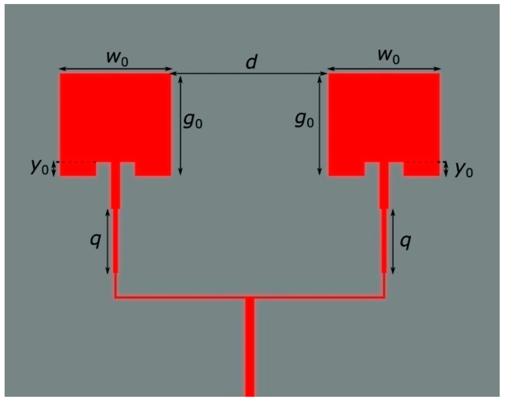
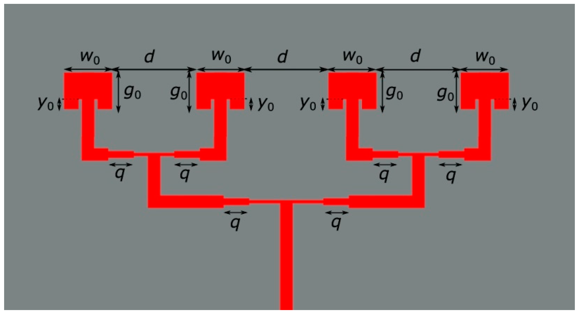
One of the main tasks on the way to derive the stochastic ANN model of a manufactured ordinary patch antenna was to estimate the geometrical uncertainty of the manufacturing process. Hence, two patch antenna arrays were designed and manufactured in a series—the first one for the C-band, and the second for the X-band and Ka-band. They are presented in Figure 1, Figure 2 and Figure 3.

The designs contain copper ground and antenna layers and an FR4 substrate layer between the copper layers. The substrate has a relative permittivity equal to 4.4 and a nominal height equal to 1.5 mm. The main geometrical design parameters are g₀, w₀, y₀, d, and q. The number of the manufactured antenna arrays for each design is 85. The antenna arrays were made by more than 10 different manufacturers.

The nominal values of design parameters for the case of the antenna arrays from Figure 1 and Figure 2 are y₀ = 2.5 mm, g₀ = 20.0 mm, w₀ = 21.6 mm, d = 30.0 mm, and q = 12.0 mm, and y₀ = 1.4 mm, g₀ = 5.1 mm, w₀ = 6.7 mm, d = 5.5 mm, and q = 3.6 mm, respectively. The author performed a comprehensive sensitivity analysis of the variation of the design parameters on the reflection coefficient for the above-presented antenna arrays. In particular, the Sobol indices analysis [16] was conducted. 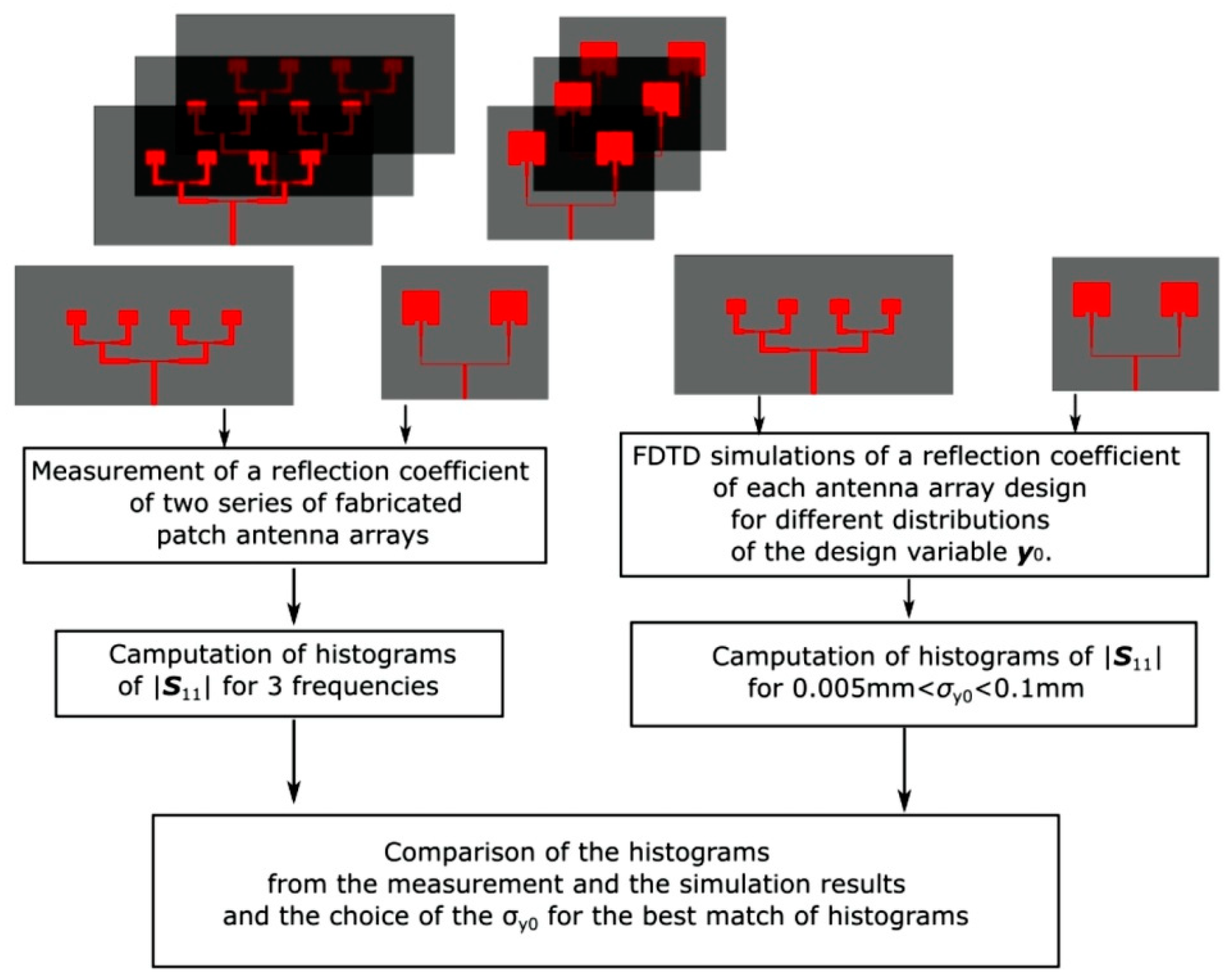The analysis concluded that the only parameter whose uncertainty had a meaningful impact on the variance of the reflection coefficient of the designed antenna arrays was y₀. Hence, the procedure for the extraction of geometrical uncertainty of the manufacturing process can be illustrated, as in Figure 4.

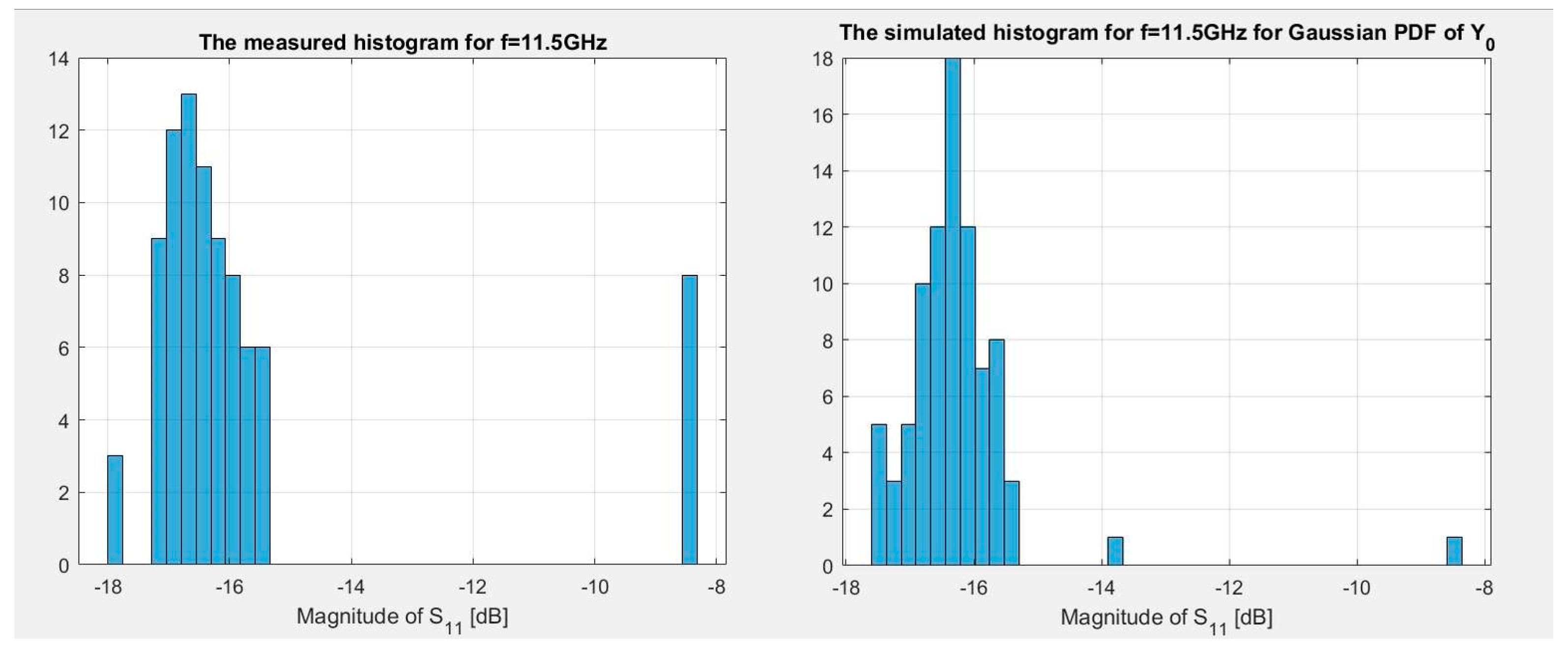
In this procedure, a histogram of measurement results is compared with histograms of the |S₁₁| simulation results obtained for different PDFs of y₀. The histogram-matching analysis was performed for y₀ having Gaussian, Beta, as well as Uniform distribution. For the case of the Gaussian distribution, the value of ${\sigma }_{y0}$ —the standard deviation of y₀ was the subject of the analysis. To make a reliable comparison of histograms for the three aforementioned PDFs, the support of Beta and Uniform distributions were $-3.5{\sigma }_{y0}\le y_0\le 3.5{\sigma }_{y0}$. 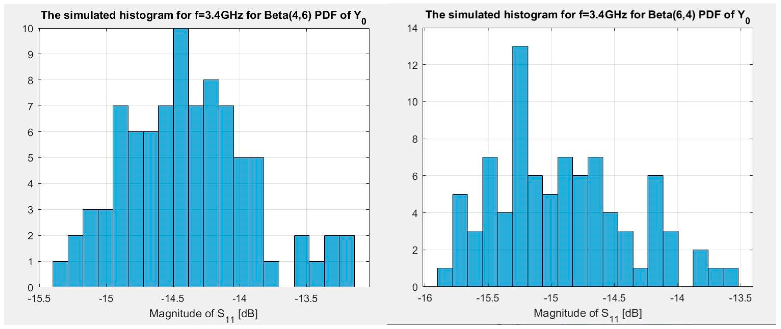Three shapes of Beta PDF were considered, one symmetrical and two asymmetrical. The symmetrical one had shape parameters α = 6, β = 6. This PDF is close in shape to the Gaussian PDF. The shape parameters α = 4, β = 6 and α = 6, β = 4 were applied to the asymmetrical Beta PDFs. Unknown σ_y0 was searched with a step equal to 0.001 mm in the range $0.005 \mathrm{mm}\le {\sigma }_{y0}\le 0.1 \mathrm{mm}$. 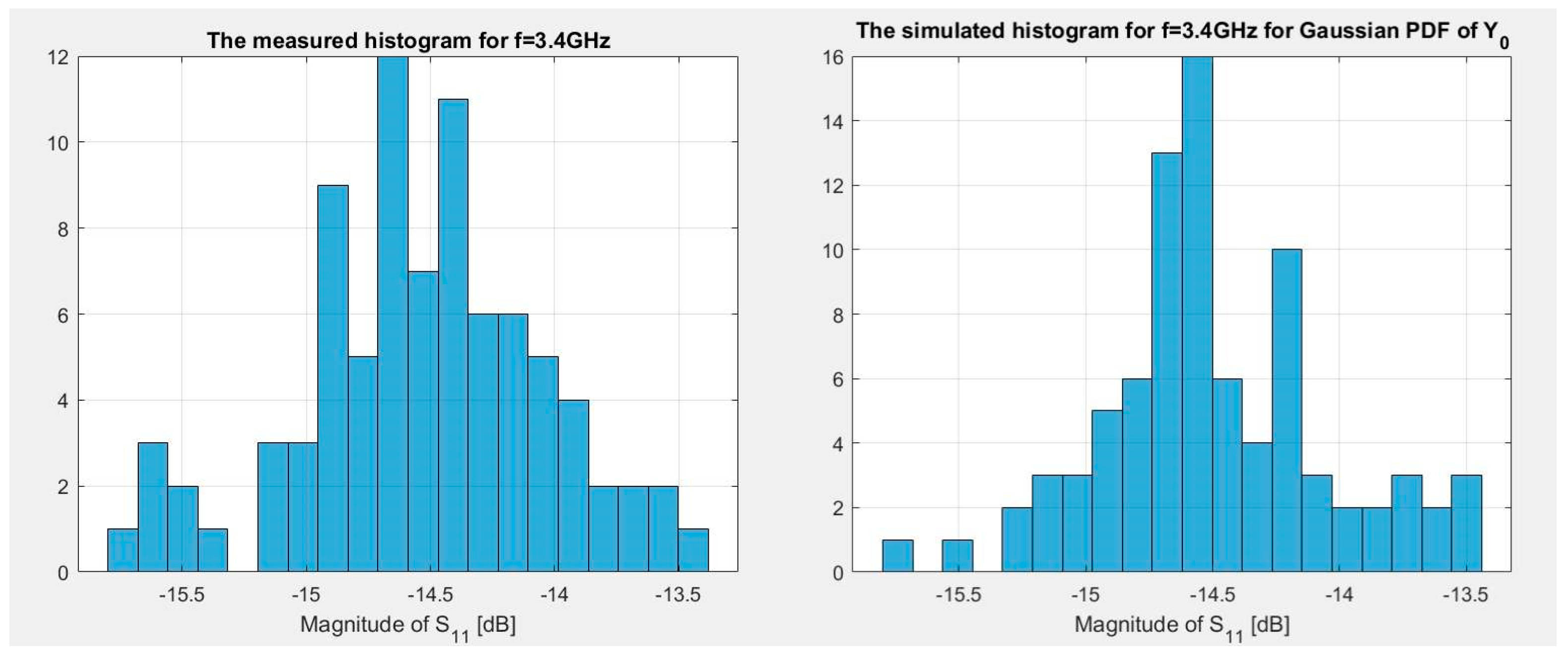This procedure was repeated for frequencies 3.4, 11.5, and 34.5 GHz. The comparison was made using an “eye-view” analysis. The author compared the shape and spread of the histograms. It turned out that the best match of the measurement with simulation results for three considered frequencies occurs when PDF of y₀ is assumed to be Gaussian, while $0.023 \mathrm{mm}\le {\sigma }_{y0}\le 0.025 \mathrm{mm}$. 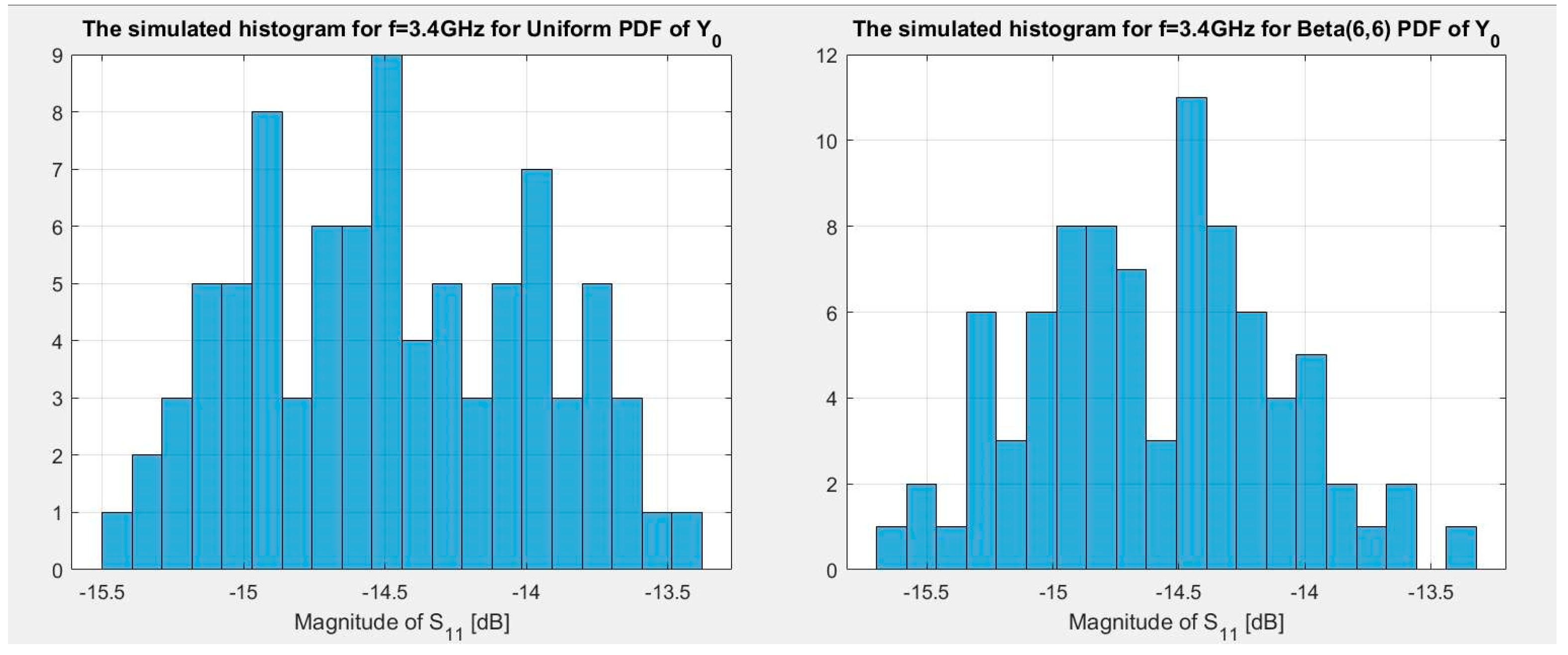A comparison of the histograms for the best match case for frequencies 3.4, 11.5, and 34.5 GHz is presented in Figure 5, Figure 6 and Figure 7. The exemplary simulation results for the case of y₀ having Uniform and Beta distribution are presented in Figure 8 and Figure 9. It can be observed that Beta distribution with shape parameters α = β = 6 can be a second choice PDF of y₀; however, the first choice is the Gaussian PDF. It should be noted that the method of comparison of histograms can be applied to antenna designs other than those from Figure 1 and Figure 2.

The estimated geometrical uncertainty of the manufacturing process is used in the next section of the paper.

3. Computation of Data for ANN Training and Testing

This section presents an application of the author’s method from [15] to the FDTD-PCE computations of data for training and testing of ANNs that are used to model the stochastic behavior of |S₁₁| of an ordinary patch antenna. The following notation is used in the paper. Random variables are denoted with bold font, vectors with capital letters, the values of variables or constants with a regular font, and variables with an italic font. An exception from this rule is the S₁₁ parameter, which is denoted in the literature by a capital letter.

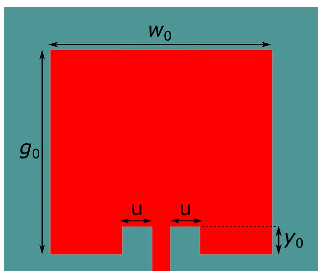
Before the presentation of the novel application of the method from [15] to the FDTD-PCE computations of training and testing data for the ANNs, let us remind the design parameters of an ordinary patch antenna, whose arrays are shown in Figure 1 and Figure 2. These parameters are denoted by g₀, w₀, and y₀ and recalled in Figure 10. The width of each inset, denoted by u, is not considered as a design variable. Its variation has a marginal effect on the |S₁₁| changes. It is considered as a constant equal to 0.5 mm. The author uses the technical data of the RT/Duroid 5880LZ with substrate thickness equal to 0.254 mm and relative permittivity equal to 2. The width of the microstrip is 0.58 mm to obtain the 50 Ω characteristic impedance of the feeding line. The three aforementioned parameters are also not treated as design variables. They remain constants for all the considered designs.

Hence, the input data for training and testing of ANNs include three variables. The author conducted a sensitivity analysis of |S₁₁| on the variations of these three aforementioned design variables in the limits corresponding to the geometrical uncertainty associated with the manufacturing process given in the previous section. The Sobol indices up to the second order were applied to quantify these impacts, as in [16]. The conclusion of the analysis is as follows. Within the considered uncertainty, variable g₀ has a marginal impact on |S₁₁|. A little higher impact is associated with variable w₀. However, the variations of them both have an overall influence on |S₁₁|, which corresponds to less than 3% of the whole variance of |S₁₁|. This observation is reflected in the details of the presentation of the novel application of the method from [15] to the FDTD-PCE computations in the following paragraphs. The author takes advantage of the fact that each nominal value of g₀ corresponds to a nominal resonance frequency (f₀) of the antenna. Hence, the author uses vector P = {f₀, y₀, w₀} of random design variables as an input of the ANNs.

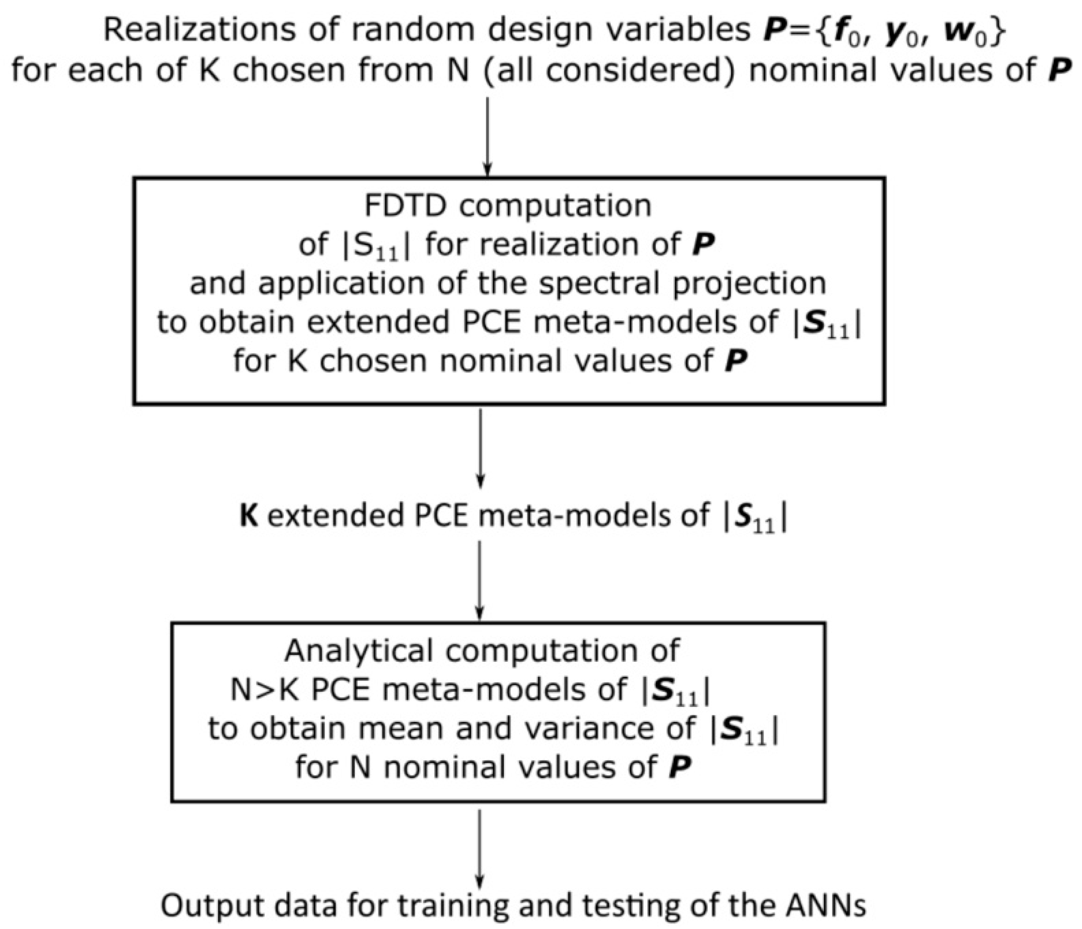
Let us assume that N nominal values of the vector of random design variables P are planned to be used as input data for the ANNs. Then, the method for the FDTD-PCE computations of the moments of |S₁₁| for training and testing of the ANNs can be presented using a diagram shown in Figure 11. By analogy to the work presented in [15], the method can be divided into two steps.

In the first step, the extended PCE meta-models of |S₁₁| for K nominal values of P are computed. The term “extended PCE meta-model” is used because this PCE meta-model is valid for the support of random design variables Ω_e, which is higher than the normal support related to the uncertainty of the manufacturing process, which can be denoted by Ω_n. In the case of this paper, the support of the extended PCE meta-model is about two times higher than Ω_n. The coefficients of the extended PCE meta-model (Equation (8) in [15]) are calculated using Beta probability distribution with the shape parameters α = β = 2.5. These values of the shape parameters of the Beta distribution were found to be optimal in terms of the quality and size of the extended PCE meta-model. It should be noted that the corresponding values of these parameters for the case of the work presented in [15] are smaller.

In the second step of the method, the author uses the extended PCE meta-models and the analytical Formulas (18), (19), (24), (25), (31), and (32) from [15] to calculate the PCE meta-models for each of N supports Ω_n associated with corresponding nominal values of design variables.

Each extended PCE meta-model is derived with FDTD-PCE computation using the openEMS Matlab-Based FDTD simulation tool [13] and the Matlab-based package called UQLab [14].

The idea of the implementation of the extended PCE meta-model is to reduce the number of required FDTD-PCE computations. Each such computation contains 11 and 16 FDTD simulation runs for supports Ω_e and Ω_n considered in this paper, respectively. The main advantage of computing the extended PCE meta-model is that all of the PCE meta-models, whose supports are included in Ω_e, can be calculated analytically. 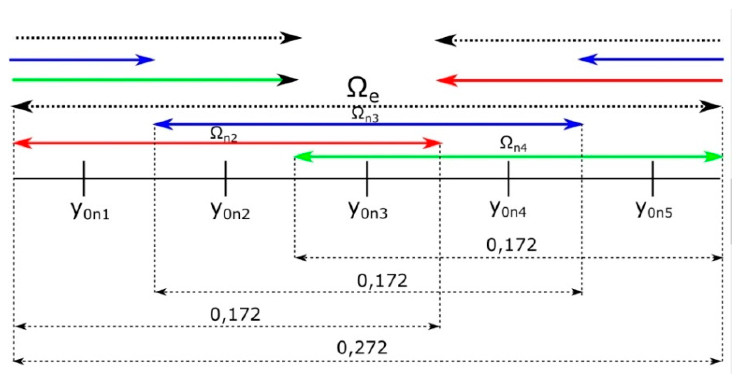Consequently, the computation of one extended PCE meta-model lets us calculate the mean and variance of |S₁₁| for more than one set of nominal design variables. Let us note that there is only one design variable whose variation has a significant impact on the change of |S₁₁|. It is the design random variable y₀. Having this in mind, the relationship between support Ω_e and support Ω_n can be presented as in Figure 12.

For the best quality of the PCE meta-models, it is assumed that the size of Ω_n is 0.172 mm, while the size of Ω_e is 0.272 mm. The nominal values of the random design variable y₀ are sampled with the step of 0.05 mm. Consequently, each FDTD-PCE computation of the extended PCE meta-model enables the calculation of three PCE meta-models for support Ω_n. Each FDTD-PCE computation takes about 45 min (16 FDTD simulation runs) using a four-core Intel platform. The corresponding computation time of the PCE meta-model with support Ω_n is about 30 min. Computations of K extended PCE meta-models require about half of the time needed to compute N PCE meta-models for support Ω_n. For example, when N equals 500 and computations are performed using one computer, then about 5 days of computation time are saved.

In the next section, the author presents ANNs that model the mean and standard deviation of |S₁₁| of an ordinary patch antenna shown in Figure 10. The data for the training of ANNs are as follows. The minimum and maximum nominal values of y₀ are 0.3 and 1.2 mm, respectively. They are sampled with a 0.05 mm step, as mentioned in the previous paragraph. The minimum and maximum nominal resonance frequencies are 24.8 GHz and 28.4 GHz, respectively. They are sampled with a 600 MHz step, which is also the approximate bandwidth of the antenna. The nominal values of g₀ are 4, 3.9, 3.81, 3.72, 3.64, 3.54, and 3.46 mm, and they correspond to the nominal values of f₀: 24.8, 25.4, 26.0, 26.6, 27.2, 27.8, and 28.4 GHz, respectively. Finally, the nominal values of w₀ are defined as the nominal values of g₀ increased by 0.1, 0.2, 0.4, and 0.5 mm. In total, 7 × 19 × 4 = 532 samples of the input and output data for training of ANNs are used. Then, the ANNs are tested using the data corresponding to the nominal values of w₀ equal to the nominal values of g₀ increased by 0.3 mm. These values are omitted in the process of training of ANNs. Furthermore, the ANNS are tested using the input and output data for the nominal values of f₀ and w₀ equal to 28.0 GHz and 3.71 mm, respectively, and 19 nominal values of y₀ with a 0.05 mm step, from which the minimum value is 0.325 mm and the maximum value is 1.225 mm. In total, 665 PCE meta-models are calculated using the algorithm presented in this section. Consequently, the time required for computation of data for training and testing of ANNs is reduced by about 6.8 days for the case of the computation on one Intel four-core platform.

4. ANNs Modeling the Random Reflection Coefficient of an Ordinary Patch Antenna

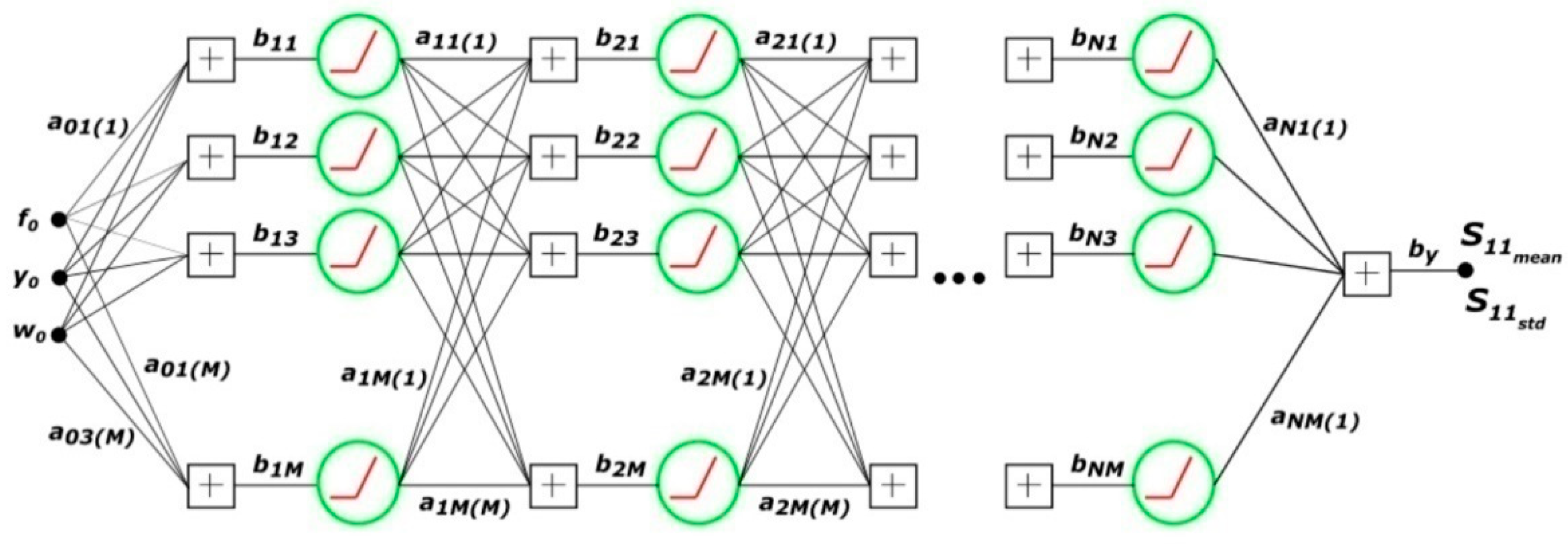
In this section, the author presents the experiments and their results corresponding to the derivation of ANNs that model the mean and standard deviation of |S₁₁| of an ordinary patch antenna shown in Figure 10. He conducted numerical experiments with the structure of ANN_S shown in Figure 13.

As a result, two separate ANNs were derived. The first one models the mean of |S₁₁|. The standard deviation of |S₁₁| is modeled by the second ANN. Each ANN contains fully connected layers of neurons. The number of ANN layers is denoted by N, while the number of neurons in each ANN layer is denoted by M. Each neuron is associated with the ReLu activation function. The bias is used before each of the neurons and directly before ANN output.

The initial values of weights are chosen using uniform random distribution in the range from 0 to 1. Input data are not normalized. The nominal values of f₀, y₀, and w₀ are put at the input of ANN using the number of GHz, mm, and mm, respectively. In the case of the training data described in the last paragraph of the previous section, the order of the input data can be illustrated as follows:

$$X_{train}=\left[\begin{array}{ccc}24.8& \dots & 24.8\\ 4.1& \dots & 4.1\\ 1.2& \dots & 0.3\end{array} \begin{array}{ccc}24.8& \dots & 24.8\\ 4.2& \dots & 4.2\\ 1.2& \dots & 0.3\end{array} \begin{array}{ccc}\dots & 24.8& 25.4\\ \dots & 4.5& 4.0\\ \dots & 0.3& 1.2\end{array}\dots \right]$$

(1)

The learning rate of the values of weights and biases of ANNs is controlled using the ADAM algorithm [22], in which values of weights and biases (denoted by θ in the ADAM algorithm) are updated in each time step t according to the formula:

$${\mathit{\theta }}_t={\mathit{\theta }}_{t-1}-\mathsf{\alpha }·\widehat{{\mathit{m}}_t}/\left(\sqrt{\widehat{{\mathit{\vartheta }}_t}}+\mathsf{ϵ}\right),$$

(2)

where:

$$\widehat{{\mathit{\vartheta }}_t}={\mathit{\vartheta }}_t/\left(1-{\mathsf{\beta }}_2{}^t\right),$$

(3)

$$\widehat{{\mathit{m}}_t}={\mathit{m}}_t/\left(1-{\mathsf{\beta }}_1{}^t\right),$$

(4)

$${\mathit{\vartheta }}_t={\mathsf{\beta }}_2·{\mathit{\vartheta }}_{t-1}+\left(1-{\mathsf{\beta }}_2\right)·{\mathit{g}}_t{}^2,$$

(5)

$${\mathit{m}}_t={\mathsf{\beta }}_1·{\mathit{m}}_{t-1}+\left(1-{\mathsf{\beta }}_1\right)·{\mathit{g}}_t,$$

(6)

$${\mathit{g}}_t={\nabla }_{\mathit{\theta }}{\mathit{f}}_{\mathrm{t}}\left({\mathit{\theta }}_{\mathrm{t}-1}\right),$$

(7)

where ${\mathit{g}}_t$ is the random nature gradient of the cost function at time step t, while α, β₁, and β₂ are the parameters whose values should be adjusted. The following cost function is used:

$$MS{E}_{\left(\mathrm{y},y^{\prime }\right)}=\frac{{{\displaystyle \sum }}_{\mathrm{i}=1}^{\mathrm{W}}{\left({\mathrm{y}}_i-{y_i}^{\prime }\right)}^2}{\mathrm{W}},$$

(8)

where y_i is the expected (training or testing data) value, while y_i′ is the estimation given by ANN.

The function of the reflection coefficient of an ordinary patch antenna is characterized by deep local minima. These minima are deeper than those experienced, e.g., in [19]. The author performed many numerical experiments to find the best ANN candidates for modeling the mean and standard deviation of |S₁₁|. Consequently, the following conclusions were made. The best results of the approximation of the mean of |S₁₁| are obtained for the values of β₁, β₂, and α equal to approximately 0.99, 0.999, and 0.001, respectively. The optimal batch size is 20–40. For the case of the approximation of the standard deviation of |S₁₁|, α = 0.005 is a better choice. The optimal number of the ANN layers for the mean of |S₁₁| is 9. The corresponding number for the standard deviation of |S₁₁| is 7. In both cases, the optimal number of neurons in each of ANN layers is about 20; however, for the case of the standard deviation of |S₁₁|, it should be slightly less, e.g., 18. The value of parameter ϵ in (2) equals 10⁻⁸. 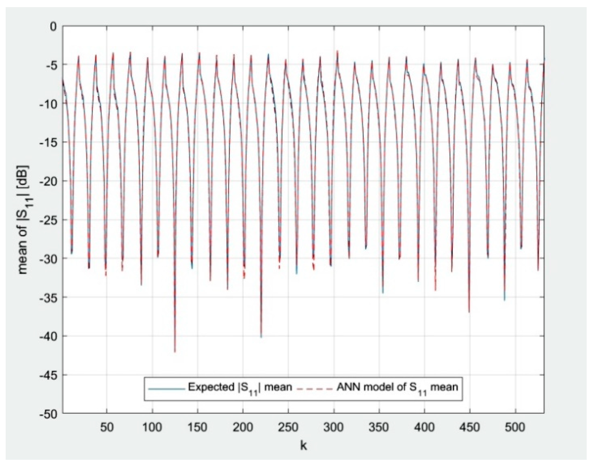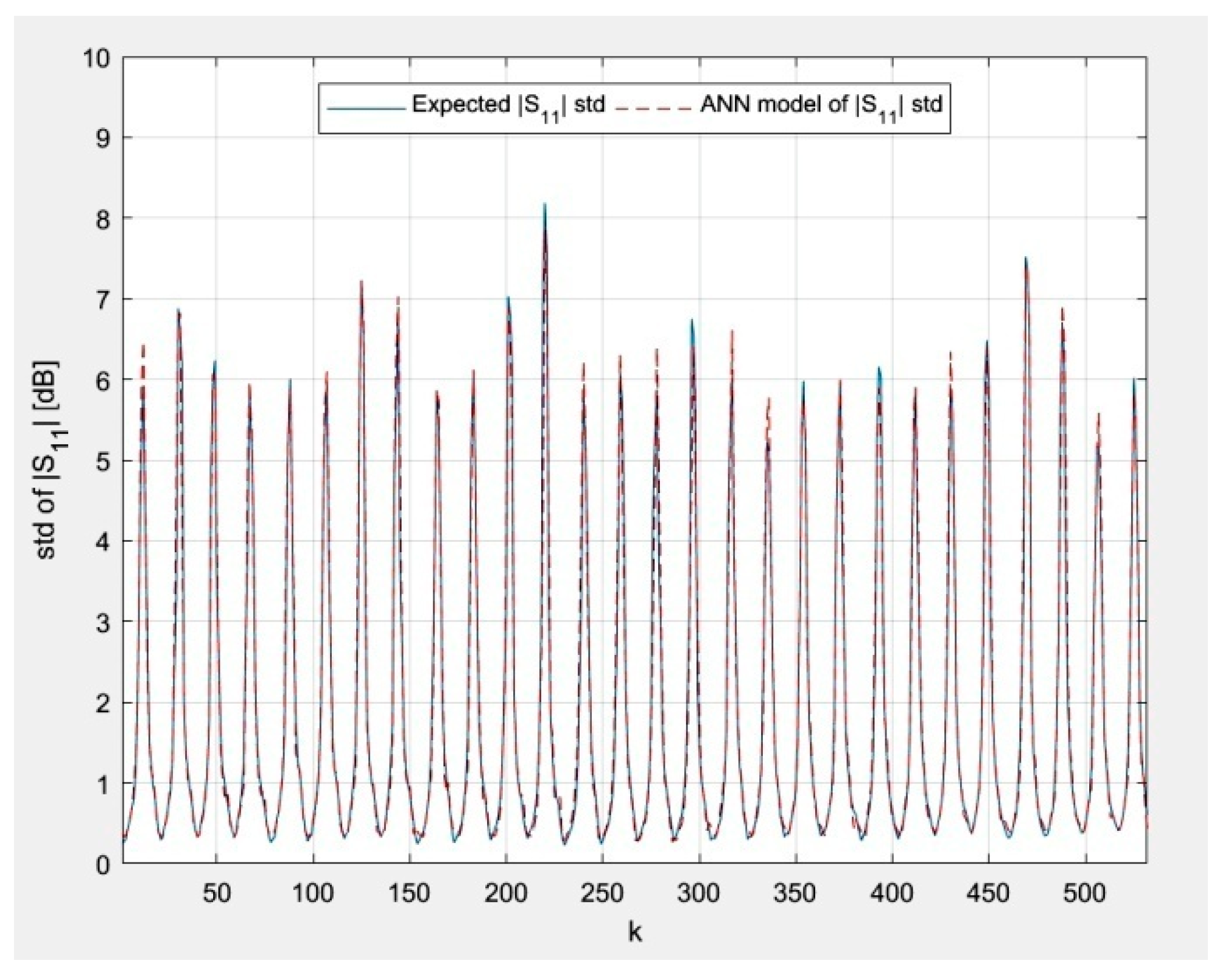It was also observed that the algorithm of SGD with Replacement [20] enables us to obtain much better approximation results than the approach with Random Reshuffling [20,21]. The experiments were performed in the Matlab environment. In the Matlab script, the author controls the average relative error of approximation and saves the optimal weights and biases in the time step when a relative error of approximation is smaller than the current smallest one. Finally, the following results for modeling the mean and standard deviation of the random reflection coefficient of an ordinary patch antenna are obtained. The results of the modeled mean and standard deviation of |S₁₁| for the training data described in the last paragraph of the previous section are shown in Figure 14 and Figure 15, respectively. The corresponding results for the testing data using nominal values of P associated with nominal values of w₀ equal the nominal value of g₀ increased by 0.3 mm are presented in Figure 16 and Figure 17. The results corresponding to the nominal value of f₀ equal to 25.4 GHz are not shown in Figure 16 and Figure 17 due to corruption of the file in which the data was saved. The order of data samples follows the rule indicated in (1).

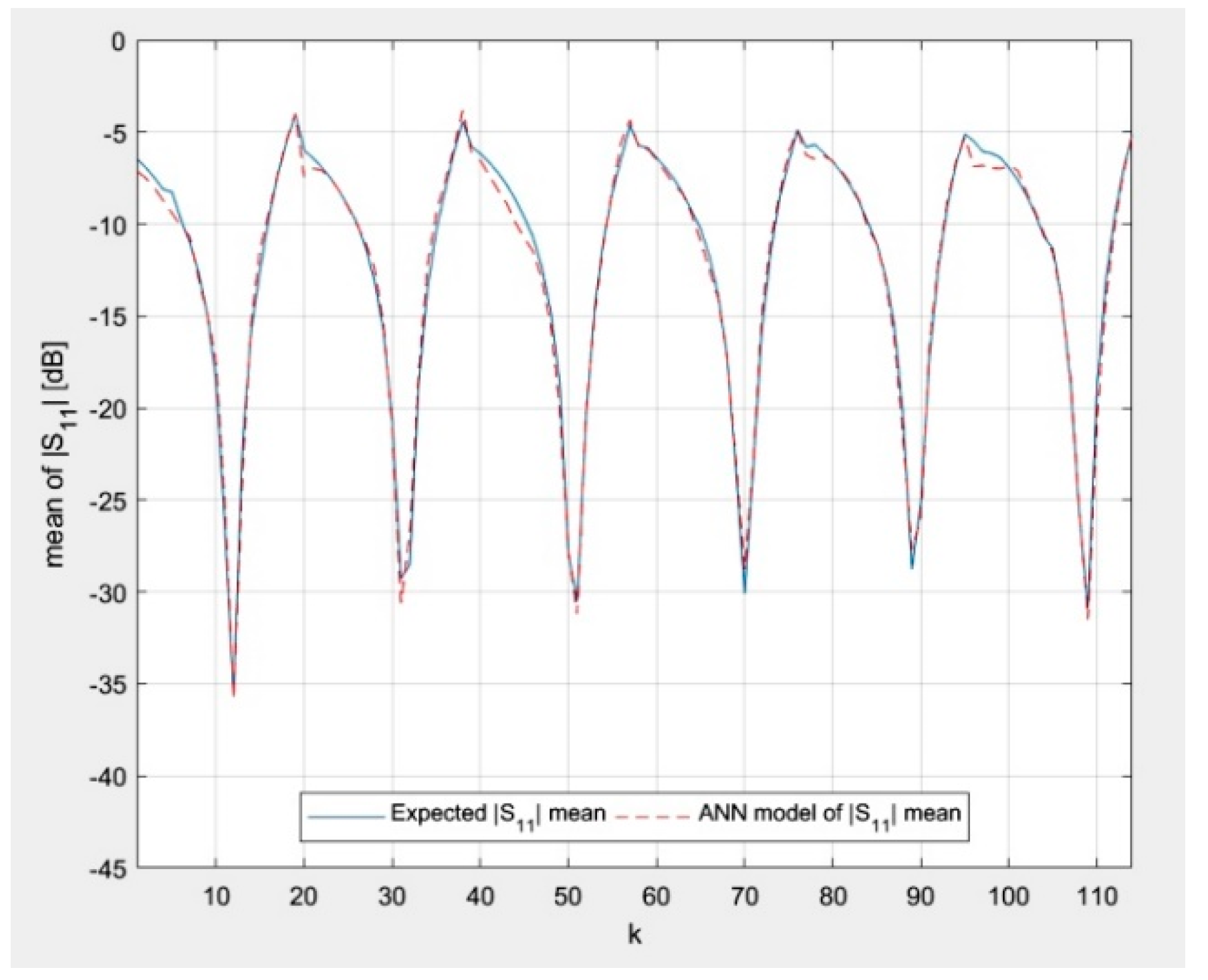
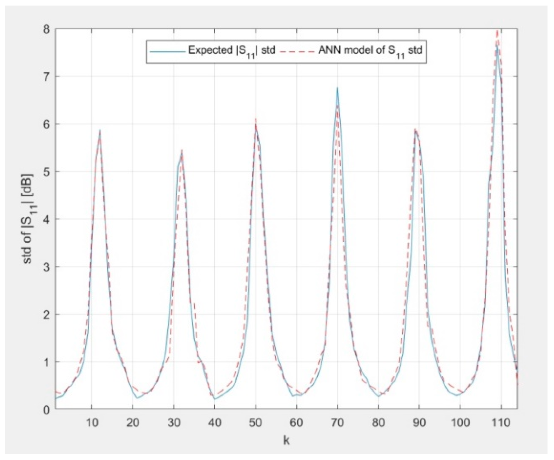
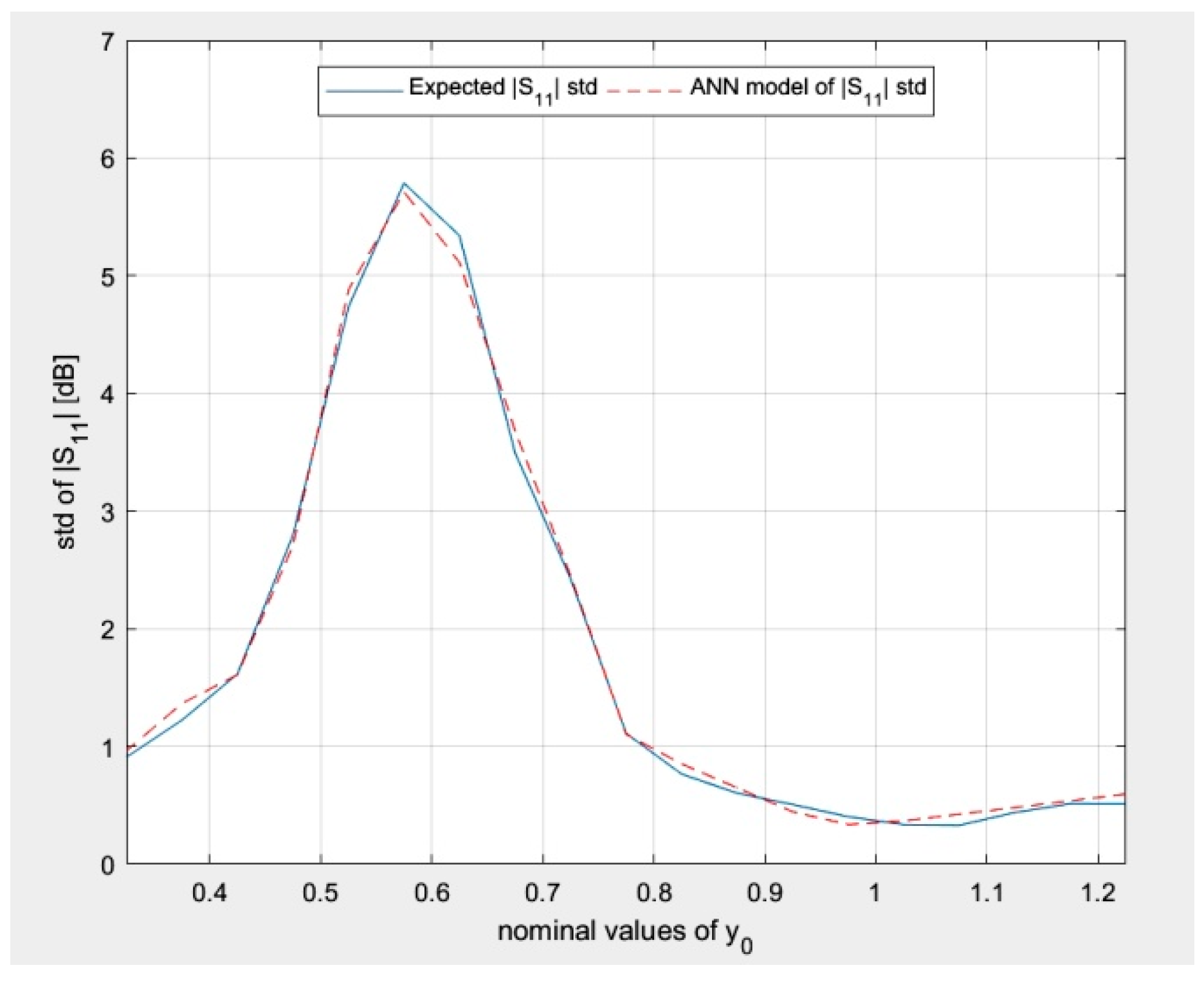
Finally, the expected and modeled mean and standard deviation of |S₁₁| for the testing data corresponding to nominal values f₀ and w₀ equal 28.0 GHz and 3.71 mm, respectively, and 19 nominal values of y₀ with a 0.05 mm step are presented in Figure 18 and Figure 19.

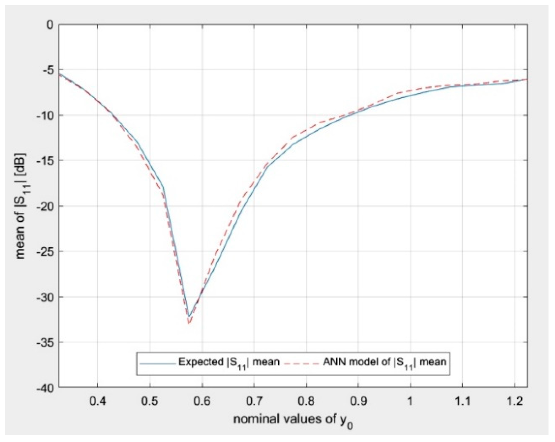
In Figure 14, Figure 15, Figure 16, Figure 17, Figure 18 and Figure 19, the author presents the novel results of modeling the random reflection coefficient of an ordinary patch antenna under geometrical uncertainty associated with the manufacturing process. It can be seen that the results of ANN modeling agree with the expected results. The model can be used for rapid optimization of ordinary patch antenna designs in terms of the geometrical uncertainties associated with the manufacturing process. The model is valid for training data and the values of parameters within the training data range. The work that is the closest to the content presented in this paper can be found in [19], where ANN modeling of deterministic S parameters is the subject of the study. It can be observed that the authors of [19] found the same optimal number of neurons in the ANN layer as in this work; however, the variation of input data is much stronger in the case of this paper. The Matlab format data containing the weights and biases of the derived ANNs can be downloaded from [23].

5. Conclusions

In the paper, the following novel results are given. Firstly, the author presents a novel method of FDTD-PCE computations for the case when the ANN is trained using stochastic input data. The novel method of FDTD-PCE computations enables saving a great amount of time. The absolute time reduction of FDTD-PCE computations can be counted in days. Secondly, the novel results of modeling the random reflection coefficient of an ordinary patch antenna under geometrical uncertainty of the manufacturing process using ANNs are presented and provided online in a Matlab format. The ANNs are derived for a wide range of resonance frequencies from n257 and n258 bands. The simple form of an ordinary patch antenna reflects the time required for computations of the PCE meta-models. This time is expected to be longer for the case of more complex antennas. The author plans to continue his work with ANN modeling in the area of antenna design and electromagnetic wave propagation.