1. Introduction
With the development of big data, cloud computing, artificial intelligence, and other technologies, the data size of networks has witnessed fast growth, and as a result, it has been more common to solve optimization problems that are similar to traffic networks, such as vehicle route planning, spacecraft design, and wireless sensor layouts [
1]. Usually, these optimization problems can be expressed with mathematical programming forms. For general simple optimization problems, mathematical programming and iterative algorithms may be used for complex large optimization problems, however, it is quite difficult to seek a global or approximate optimal solution within a reasonable time with these traditional methods. Therefore, to smoothly solve complex large optimization problems, the heuristic algorithm was proposed and has received increasing attention in recent decades [
2].
In computer science and mathematical optimization, a metaheuristic is a higher-level procedure or heuristic designed to find, generate, or select a heuristic that may provide a sufficiently good solution to an optimization problem, especially with incomplete or imperfect information or limited computation capacity [
3,
4]. The common meta-heuristic algorithms include a genetic algorithm, simulated annealing algorithm, and particle swarm optimization algorithm [
5,
6]. Unlike meta heuristics, which are independent of the problem, heuristic algorithms depend on a specific problem. Heuristic algorithms are essentially methods by trial and error [
7]. In the process of seeking the optimal solution, it can change its search path according to individual or global experience. When it becomes impossible or difficult to find the optimal solution of the problem, a heuristic algorithm is an efficient method to obtain the feasible solution [
8]. Harmony search is a heuristic global search algorithm introduced in 2001 by Zong Woo Geem, Joong Hoon Kim, and G. V. Loganathan [
9]. Inspired by the improvisation of musicians, it simulates musicians’ improvisation process to achieve subtle harmonies. The HS algorithm is characterized by merits such as a simple structure, less demand for parameters, a high convergence rate, and strong robustness, which facilitates its application in optimizing a system’s continuous and discrete variables [
10]. We hope that the HS algorithm can effectively solve some optimization problems. In recent years, scholars have constantly improved the algorithm and made some progress [
11,
12,
13,
14].
Mahdavi et al. used a new method for generating new solution vectors and set the pitch adjustment rate and distance bandwidth as dynamic changes, improving the accuracy and convergence rate of the HS algorithm [
15]. Khalili et al. changed all key parameters of the HS algorithm into a dynamic mode without predefining any parameters. This algorithm is referred to as the global dynamic harmony search, and such modification imbued the algorithm with outstanding performance on unimodal functions and multimodal functions [
16]. In view of the drawbacks of HS such as a low convergence rate and solving accuracy in solving complex problems, Ouyang et al. proposed an adaptive global modified harmony search (MHS) that fuses local searches [
17]. Pan et al. proposed the concepts of the maximum harmony memory consideration rate, the minimum harmony memory consideration rate, the maximum regulation bandwidth, the minimum regulation bandwidth, etc. on the basis of the standard HS algorithm, and they achieved an automatic regulation mechanism for the relevant parameters of the harmony search algorithm by improving the current harmony memory consideration rate for each iteration and changing the bandwidth with the number of iterations [
18]. To improve the efficiency of the HS algorithm and make up for its drawback of easily getting into local search, Zhang Kangli et al. improved the generation of the initial solution vector’s harmony memory and proposed an improved harmony algorithm, ALHS [
19]. Given the low evolution efficiency of single populations and fewer studies on multi-population improvement, S. Z. Zhao combined dynamic multi-swarm particle swarm optimization (DMS-PSO) with the HS algorithm and simplified it into the dynamic multi-swarm particle swarm optimization harmony search (DMS-PSO-HS). These sub-populations are frequently re-combined, and there is information exchange among particles in the entire population. Compared with DMS-PSD and HS, DMS-PSO-HS is improved from the aspect of multi-mode and combinatorial testing [
20]. As to the problems with the HS algorithm in solving high-dimensional multi-objective optimization problems, Zhang proposed an improved differential evolved harmony search algorithm. In this algorithm, mutation and crossover are adopted to substitute the original pitch adjustment in the HS optimization algorithm, thus improving the global search ability of the algorithm [
21]. To effectively solve integrated process planning and scheduling (IPPS) problems, Wu et al. proposed a nested method for single-objective IPPS problems. On the external layer of the method, the HS algorithm was used to determine the manufacturing feature processing sub-path, and static and dynamic scoring methods were proposed for the sub-path to guide the search on the external layer. Meanwhile, a genetic algorithm was adopted on the internal layer to determine machine allocation and operation series. Upon combining the two algorithms, the validity of the proposed method was proved through a test of benchmark instances [
22].
Inspired by the above, the improvement of the HS algorithm mainly focuses on the improvement of parameters and infusion with other algorithms. In this paper, to solve the main problems with the algorithm, such as its poor global search ability and poor solution accuracy, a reward population-based differential harmony search algorithm is proposed. The highlight of the proposed algorithm is as follows. (a) We hope that by using the multiple population reward mechanisms, the population diversity can be increased and the algorithm can avoid falling into local optimization as much as possible. (b) In the step of generating a new harmony, excellent individuals in existing populations are utilized for optimization, thus improving the convergence rate of the algorithm; at the same time, on the basis of differential evolution and genetic operations, the difference among individuals is utilized flexibly for search guidance, thus improving the search ability of the algorithm. Finally, in a numerical experiment, the validity of the algorithm is verified through comparison.
2. Harmony Search Algorithm
The harmony search algorithm is a novel intelligent optimization algorithm. Like the genetic algorithm, which simulates biological evolution, the simulated annealing algorithm, which simulates physical annealing, and the particle swarm optimization algorithm, which simulates flocks of birds, the harmony algorithm simulates the principle of concert performances [
23].
Let us assume that a band consists of n people, and everyone plays a specific musical instrument. Then, all sounds being played correspond to a group of harmonies after combination, which is: . As the tone of the initial harmony is not necessarily the best, they need to get the best harmony through continuous cooperation and rehearsal. For convenience of comparison, a mathematical function can be used to measure whether a harmony sounds good in the whole process. The serves as a general director, as well as a general judgment criteria. If the requirements are not met, the performance should be constantly adjusted until a set of satisfactory harmonies is achieved. This is the optimization process of the harmony search algorithm.
2.1. Parameters Involved in Harmony Search Algorithm
In short, for the harmony search algorithm (HS), all solution vectors (decision variable sets) are stored in harmony memory (HM). The main parameters of the HS algorithm are the harmony memory size (HMS), harmony memory consideration rate (HMCR), pitch adjusting rate (PAR), distance bandwidth (BW), and number of improvisations or stopping criterion (NI).
Harmony memory size (HMS): As the music of each musical instrument has a specific range, a solution space may be constructed on the basis of such a performance range. Then, the solution space is used to generate a harmony memory randomly. Therefore, the size of the harmony memory should be designated first.
Harmony memory consideration rate (HMCR): In each iteration, a set of harmonies should be extracted from the harmony memory at a specific rate. Upon micro tuning the set, a set of new harmonies is obtained. Then, a judgment is made on whether the new harmonies are better than the worst harmony in the harmony memory. The process of this judgment involves a comparison done on the basis of the function mentioned above. Therefore, a random harmony memory consideration rate should be generated.
Pitch adjusting rate (PAR): A set of harmonies should be selected from the harmony memory at a specific consideration rate for pitch adjustment.
Tone pitch adjusting bandwidth (BW): As mentioned above, a set of harmonies will be selected from the memory for pitch adjustment at a specific consideration rate. Bandwidth (BW) refers to the adjustment amplitude.
Maximum times of creation (): This refers to the times of creation by concert performers, or namely, the number of times the whole harmony adjustment process needs to be repeated.
2.2. Flow of Harmony Search Algorithm
(1) Initialize the problem and algorithm parameters
In general, the global optimization problem can be summarized as follows. Minimize
subject to
where,
is the objective function,
x is the set of the decision variables
,
N is the number of decision variables,
is the set of possible ranges of values for each decision variable, the upper bound for each decision variable is
, and the lower bound is
; then
.
In
Section 2.1, it was introduced that five parameters are involved in harmony research. At the very beginning of the algorithm, these values should be set properly.
(2) Initialize harmony memory
A harmony memory with a size of HMS is generated on the basis of the solution space, as follows.
Each decision variable is generated as follows: for and , where r is a random number between 0 and 1.
(3) Generation of new harmony
A new harmony vector is generated by three rules: (a) memory consideration, (b) pitch adjustment, and (c) random selection [
24]. First, randomly generate a random number
in the range [0,1] and compare
with the initialized HMCR. If
, take a variable randomly from the initialized HM, which is called memory consideration. Otherwise, it can be obtained by random selection (i.e., randomly generated between the search boundaries). In the last step, take a new harmony variable. If it is updated by the memory consideration, it needs to be adjusted, and a variable
between [0,1] is randomly generated. If
, adjust the variable on the basis of the initialized BW and get a new variable, which is called pitch adjustment. The pitch adjustment rule is given as:
where
r is a random number between 0 and 1.
(4) Update of harmony memory
The newly obtained harmony is calculated with . If the new harmony has a better objective function solution than the poorest solution in the above initialized harmony memory (HM), the new harmony will substitute the poorest harmony in the harmony memory.
(5) Judgment on termination
Check whether current times of creation have reached the above initialized maximum times of creation. If no, Steps 3–4 should be repeated until the maximum times of creation are reached.
The complete steps of the harmony search algorithm are shown in Algorithm 1.
| Algorithm 1: HS Algorithm |
| 1: | Initialize the algorithm parameters HMS, HMCR, PAR, BW, |
| 2: | Initialize the harmony memory. |
| 3: | Repeat |
| 4: | Improvise a new harmony as: |
| 5: | for all i, do |
| 6: | |
| 7: | HM, then |
| 8: | |
| 9: | end if |
| 10: | end for |
| 11: | if the new harmony vector is better than the worst |
| 12: | one in the original HM, then |
| 13: | update harmony memory |
| 14: | end if |
| 15: | Until is fulfilled |
| 16: | Return best harmony |
3. Improved Harmony Search Algorithm
Although the harmony search algorithm has the merits of satisfactory realizability, there are still some drawbacks to be overcome, such as a poor global search ability, inadequate accuracy in dealing with high dimensional optimization problems, and difficulties in pitch adjustment [
25]. In this paper, a reward population-based differential genetic harmony search algorithm (RDEGA-HS) is proposed. Furthermore, the reward population harmony search algorithm (RHS) and differential genetic harmony search algorithm (DEGA-HS) are designed to facilitate comparison of the results in the experiment.
3.1. Reward Population Harmony Search Algorithm (RHS)
In this paper, we propose a multi-population model based on reward population. First, the initialized harmony memory is divided into multiple sub-memories, including several common sub-memories and one reward memory. The size of each memory is subject to the parameter
. Namely,
where,
and
refer to the total harmony memories and sub-harmony memories, respectively,
and
refer to the number of the total harmony memories and sub-harmony memories, respectively,
refers to the proportion of each sub-harmony memory, and
i refers to the number of sub-harmony memories.
Each harmony memory evolves separately. Furthermore, after each evolution, the sub-harmony memory with the optimal average fitness is combined with the reward harmony memory to form a new reward harmony memory. At the same time, poor harmony factors are eliminated to guarantee stability in the number of newly generated harmony memories. In this paper, four sub-harmony memories and one reward memory are set.
3.2. Differential Genetic Harmony Search Algorithm (DEGA-HS)
3.2.1. Mutation of Differential Evolution
The differential evolution algorithm (DE) is a population-based heuristic search algorithm [
26]. The flows of evolution are quite similar to those of the genetic algorithm. The operators of both are selection, crossover, and mutation. For the genetic algorithm, crossover goes before mutation. For the DE algorithm, however, mutation goes before crossover. Furthermore, with regard to the specific definition of these operations, there is a difference between the two algorithms.
Let us assume that a population consists of NP N-dimensional vector individuals. Then, each population can be expressed as: . Generally, after the initialization of a population, the differential mutation operation will generate mutation vectors. The mutation strategy of the DE algorithm is advantageous in overcoming premature convergence. Therefore, it was considered that the mutation operation of the DE algorithm be introduced into the harmony search algorithm to overcome the premature convergence of the harmony search algorithm, thus improving the convergence rate.
There are many forms of mutation operations, where the common forms are DE/rand/ 1/bin, DE/best/1/bin, DE/rand to best/1/bin, DE/best/2/bin and so on. As to the representative methods, they are “selection of DE algorithm”, “basic vector selection method”, “number of differential vectors”, and “crossover methods”. Generally, they are expressed in the form of DE/base/num/cross. If “best” is selected for the base part, it means the optimal individual from the population is selected as the basic vector; if “rand” is selected, it means random selection. If “bin” is selected for the cross part, it means binomial crossover is adopted. The results show that if “rand” is selected in the base part, it is favorable for maintaining diversity in populations; if “best” is selected, it stresses the convergence rate [
27].
For each individual
in a population, a mutation vector of the differential evolution algorithm is generated as per the following formula.
,and are selected randomly and differ from each other. is referred to as a basic vector, ( ) is referred to as a differential vector, and F is a scaling factor, . F is used to control the size of the differential vector. It is worth noting that an excessively great value of F will cause difficulties in the convergence of populations, and an excessively small value will reduce the convergence speed.
In this paper, two mutation strategies of DE are fused to improve the proposed algorithm. “DE/rand/bin” is selected randomly during iteration, without using the current optimal solution. Therefore, the convergence rate is relatively low, but the global search ability is strong. During iteration, as “DE/best/1/bin” utilizes the current optimal solution, the algorithm is able to better improve the convergence rate. On this basis, “DE/best/1/bin” is flexibly used in the memory consideration of the HS algorithm, while “DE/rand/1/bin” is used for substituting pitch adjustment in the HS algorithm. The two mutation generation strategies are as follows.
3.2.2. Partheno-Genetic Algorithm
To increase the diversity of harmony factors, the Partheno-genetic algorithm (PGA) was considered to increase the means of generating new harmonies. For individuals with high randomness, they are subject to a shift operation, inversion operation, and permutation operation, and thus, three new harmonies are obtained. Then, the harmony with the optimal fitness is selected as the new individual introduced by the genetic operation.
The PGA is an improved GA that was put forward by Li and Tong in 1999 [
28]. PGA is a genetic method for reproduction through gene shift, gene permutation, and gene inversion. Next, we will introduce genetic operators, namely, the permutation operator, shift operator, and inversion operator, which are characterized by a simple genetic operation, decreasing the requirement for diversity in the initial population and avoiding “premature convergence” [
29].
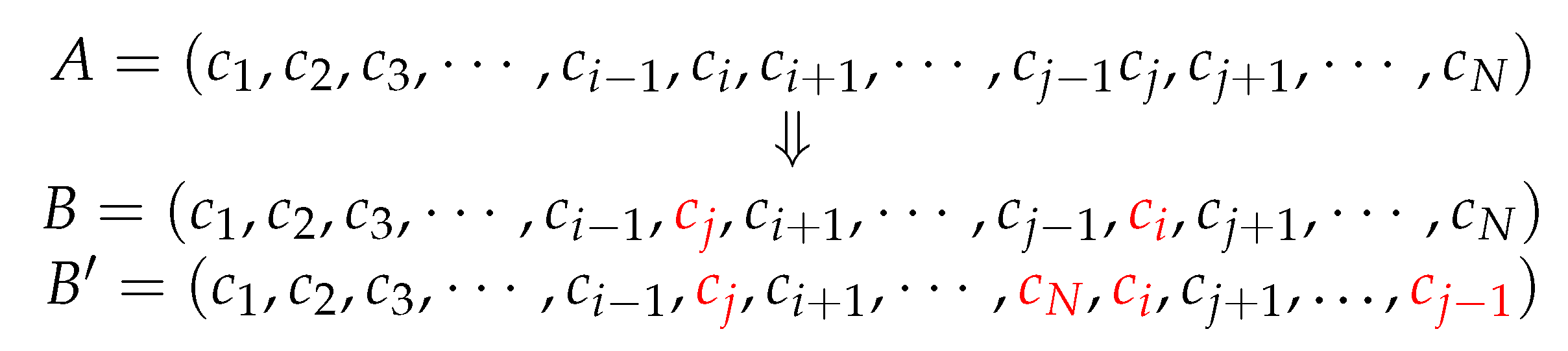
(1) Permutation Operator.
The permutation operator is a process where genes at specific locations of a chromosome are exchanged at a certain probability and the locations of the exchanged genes are random. Permutation operators may be divided into single-point permutation and multi-point permutation. As to single-point permutation, two genes on a chromosome are exchanged, and in multi-point permutation, multiple genes on a chromosome are exchanged. The process of the two permutation operators is shown in
Figure 1, where
B and
are the single-point permutation and multi-point permutation result for Chromosome
A, respectively.
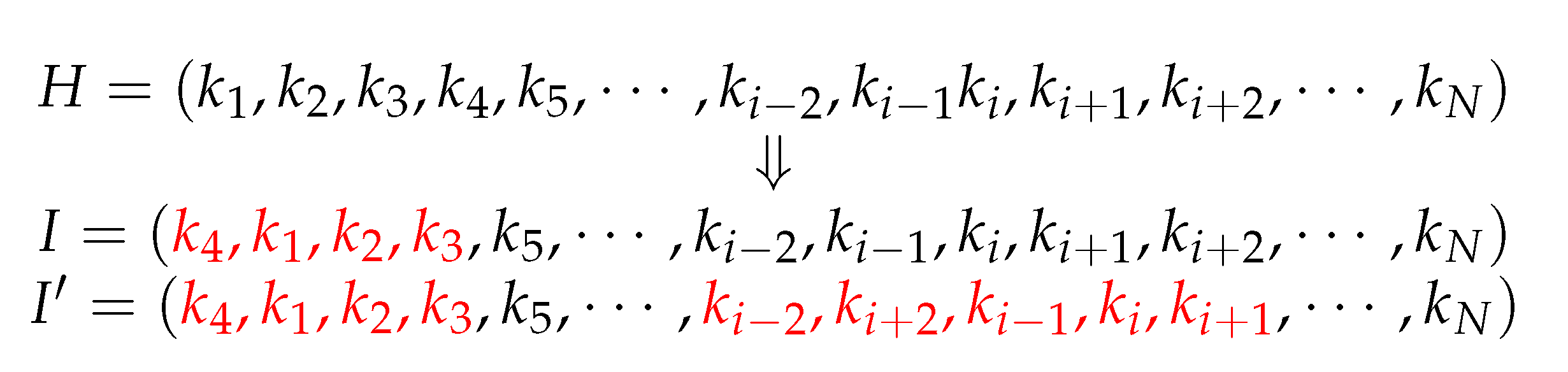
(2) Shift Operator.
The shift operator is a process in which genes in some substrings of a chromosome are shifted backward successively, while the last gene in the substring is shifted to the foremost location. The substrings whose genes are shifted in a chromosome and their length are selected randomly. The gene shift can be divided into single-point shift and multi-point shift. As to single-point shift, only one substring of a chromosome is selected for gene shift, and in multi-point shift, multiple substrings of a chromosome are selected for gene shift. The process of the shift operation is shown in
Figure 2.
H is a chromosome including multiple genes
.
I and
are chromosomes obtained by implementing single-point shift and multi-point shift operations for
H, respectively.
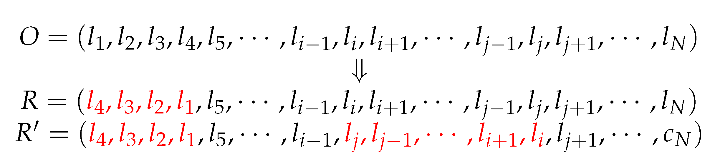
(3) Inversion Operator.
The inversion operation is a process where the genes in some substrings of a chromosome are inversed successively at a specific probability. The substrings for gene inversion in a chromosome and their length are selected randomly. The gene inversion can also be divided into single-point inversion and multi-point inversion. As to single-point inversion, only one substring of a chromosome is selected for gene inversion, and for multi-point inversion, multiple substrings of a chromosome are selected for gene inversion. The operation is shown in
Figure 3. We assume
O is a chromosome including multiple genes
. On the basis of the operations of single-point and multi-point inversions for chromosome
O, we can obtain the chromosomes
R and
.
The multi-point genetic operator is usually used when the chromosome length is large, while the single-point genetic operator is used when the chromosome length is small. Therefore, the genetic algorithms of single-point permutation, single-point shift, and single-point inversion for reproduction are used for genetic operator operations and applied to random selection in the general harmony search algorithm.
3.2.3. Flow of DEGA-HS Algorithm
As stated above, the mutation strategy of the differential mutation algorithm has the advantage of overcoming premature convergence and degeneration. Therefore, we considered introducing the mutation strategy of DE into the HS algorithm to overcome the premature convergence of HS, thus improving the convergence rate. At the same time, there is excessively high randomness in the generation of a new harmony in the general harmony search algorithm. High randomness brings both advantages and disadvantages. To balance this contradiction, the Partheno-genetic algorithm is also introduced.
The flow of the improved DEGA algorithm is as follows.
Step 1. Initialization of parameters.
In the new algorithm, the original tone pitch adjusting bandwidth (BW) will be canceled. Therefore, only the harmony memory size (HMS), harmony memory consideration rate (HMCR), pitch adjusting rate (PAR), and maximum times of creation () will be initialized.
Step 2. Random initialization of harmony memory.
Step 3. Generation of a new harmony.
For the general harmony search algorithm, there are mainly three operations to generate a new harmony at this step: memory consideration, pitch adjustment, and random selection. However, the operations of the proposed algorithm differ from them. The flow is as follows.
First, a random number is generated between (0,1). If is smaller than or equal to HMCR, the mutation strategy of “DE/best/1/bin” is used to generate a new harmony. Namely, . Then, a second random number is generated between (0,1). If is smaller than or equal to PAR, the mutation strategy of “DE/rand/1/bin” is used. Namely, . Otherwise, no adjustment is made.
If is greater than HMCR, a new harmony is generated within the search boundary. Next, a third random number is generated between (0,1). If is smaller than or equal to PAR, a new harmony is generated according to the operation of the Partheno-genetic operation. Otherwise, no adjustment is made.
Step 4. Update of harmony memory.
The newly generated harmony is assessed. If it is better than the poorest harmony in the harmony memory, substitution is made.
Step 5. Judgment on termination.
Check whether current times of creation have reached the set maximum times of creation. If no, Steps 3–4 should be repeated until the maximum times of creation are reached.
3.3. Reward Population-Based Differential Genetic Harmony Search Algorithm (RDEGA-HS)
We hope the combination of the multi-population reward mechanism with a differential genetic harmony algorithm will increase the diversity of harmony and improve the convergence rate.
The specific flow of the algorithm is as follows.
Step 1. Initialization of algorithm parameters.
Step 2. Random initialization of harmony memory.
Step 3. The total harmony memory is divided into (Q is an integer greater than 0) sub-harmony memories, including Q common sub-harmony memories and one reward sub-memory.
Step 4. As to all sub-harmony memories including the reward sub-memory, new harmonies are generated on the basis of differential genetic operations.
Step 5. Update of each sub-harmony memory.
Step 6. Judge whether the maximum number of iterations has been reached. If no, Steps 4 and 5 are repeated. Otherwise, move on to Step 7.
Step 7. Find the common sub-harmony memory with the best evolution effect at present, and combine it with the original reward harmony memory. Then, sort them from good to bad according to the fitness. On the premise of keeping the number of harmonies in the newly generated harmony memory unchanged, eliminate bad harmonies, and form a new reward harmony memory to replace the original reward harmony memory.
Step 8. Judge whether the upper limit of iteration has been reached. If yes, then exit the loop and output the optimal solution. Otherwise, return to Step 4.
The pseudo-codes of the algorithm are shown in Algorithm 2.
| Algorithm 2: RDEGA-HS Algorithm |
| 1: | Initialize the algorithm parameters |
| 2: | Initialize the total harmony memory |
| 3: | For |
| 4: | Repeat |
| 5: | While time(2) , do |
| 6: | Improvise each new harmony as follows: |
| 7: | While time(1) |
| 8: | For all j, do |
| 9: | |
| 10: | If with probability HMCR, then |
| 11: | |
| 12: | Else, do |
| 13: | |
| 14: | End If |
| 15: | End For |
| 16: | If the new harmony vector is better than the worst one in the |
| 17: | original HM, then |
| 18: | update the harmony memory |
| 19: | End If |
| 20: | End while |
| 21: | Update the reward harmony memory |
| 22: | End While |
| 23: | End For |
| 24: | Return best harmony |
4. Experiments
To carry out an in-depth study on the performance of RDEGA-HS, two experiments were carried out to determine the influence of the values of HMS and HMCR on the performance of the algorithm and to perform a comparative study between the HS algorithm and the three proposed HS algorithm variants. The function name, formulation, and search range are listed in
Table 1. In this paper, we used six benchmark functions to verify the ability of the RDEGA-HS algorithm in finding the optimal solution, so as to judge the advantages and disadvantages of the improved algorithm. Then, a comparison was made among the results of HS, RHS, and DEGA-HS.
The Ackley function is a widely used multi-mode test function. The Griewank function has many widely distributed local minimum values and is considered to be a convex function. The Rastrigin function is a high-dimensional multi-mode function; in this function, a frequent local minimum value is generated by increasing cosine modulation, and the locations of minimum values are generally scattered. In addition, benchmark functions such as Rosenbrock, Sphere, and Schwefel function are also used in the experimental steps.
4.1. Effects of HMS and HMCR on Performance of RDEGA-HS
In this section, the six benchmark functions in
Table 1 are used for studying the influence of HMS and HMCR on the performance of the algorithm. The dimensions of the six functions were set to 40. Each case was independently run 50 times.
Table 2 and
Table 3 report the average value and standard deviation obtained with different values of HMS and HMCR, respectively. In this experiment, we set the termination based on the maximum number of iterations.
is set to 10 and
is set to 100, so the maximum number of iterations is 1000.
It can be seen from
Table 2 that HMS influenced the result of the algorithm. When HMS was 80, the algorithm achieved the best optimization accuracy and stability. Therefore, HMS was set to 80 in all test experiments herein.
It can be seen from
Table 3 that the value of HMCR obviously influenced the optimization result of the proposed algorithm. A greater HMCR will obviously improve the local search ability, thus improving the performance of the algorithm. A smaller HMCR will influence the performance of the algorithm. When HMCR was 0.9, the proposed algorithm demonstrated a higher convergence rate. Therefore, in this paper, the HMCR value was chosen to be 0.9.
4.2. Comparative Study on RDEGA-HS and HS Variants
To study the expandability of the algorithm, six different variable dimensions were used in each function test: 30, 40, 50, 60, 70, and 80. In a simulation experiment, the common parameters were set as follows: HMS = 80, HMCR = 0.9, PAR = 0.6, and BW = 0.05. As in the previous experiment, we set the maximum number of iterations as the termination. Since the algorithm we proposed has two loops, in order to show fairness when compared with other algorithms, we set to 10 and to 100, so the maximum number of iterations is 1000. As a correspondence, the maximum number of iterations of the other three algorithms is also set to 1000. All optimization algorithms were achieved in Matlab R2021a.
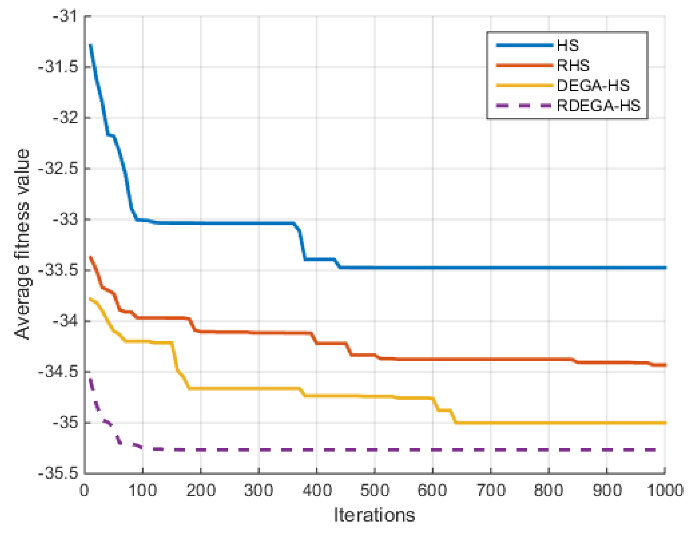
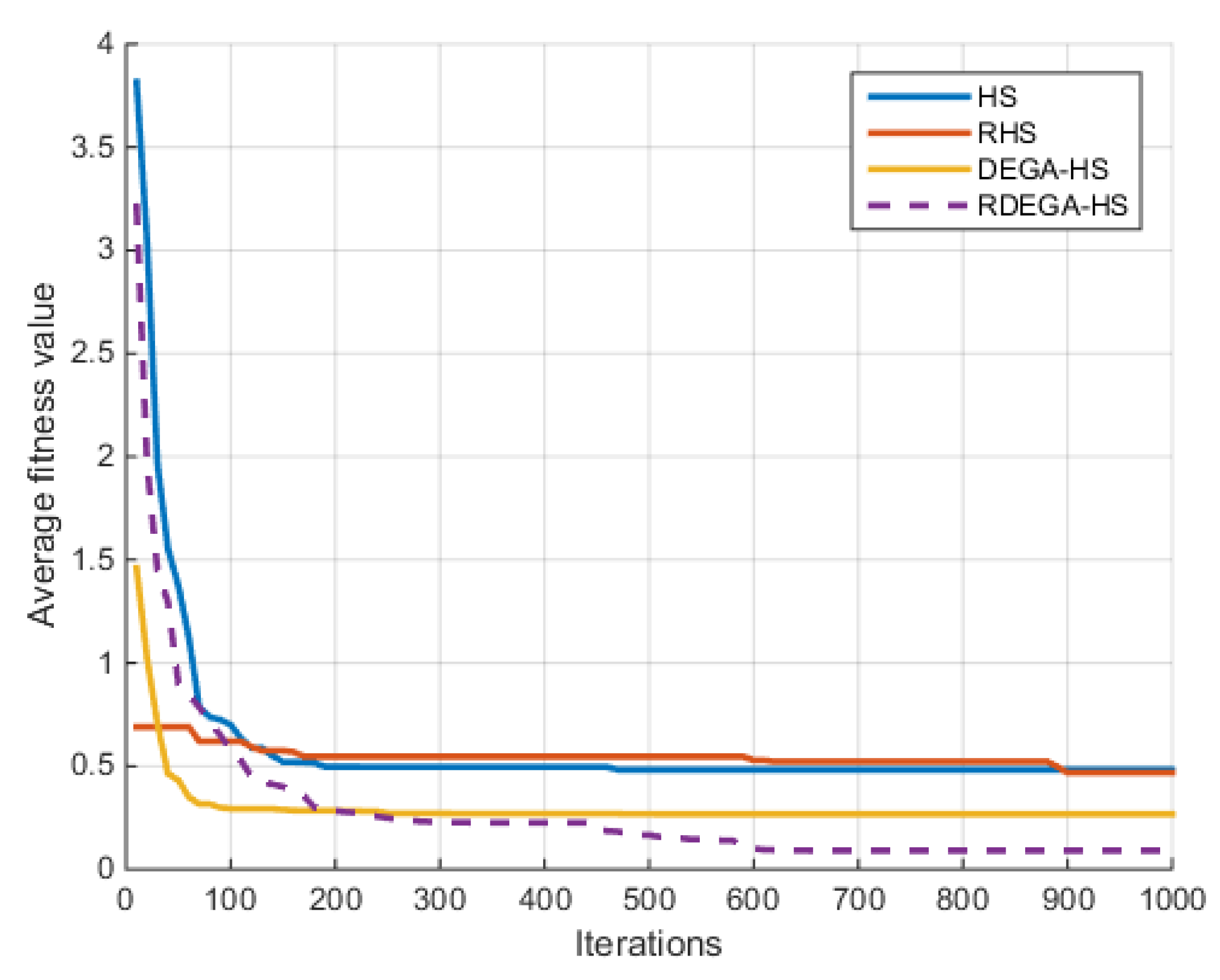
To measure the convergence accuracy, robustness, convergence rate, and other performances of the different optimization algorithms, each function was run independently for 100 times. Then, the average optimal value and standard deviation were taken to serve as the final evaluation indexes. The curve of the average optimal fitness was given.
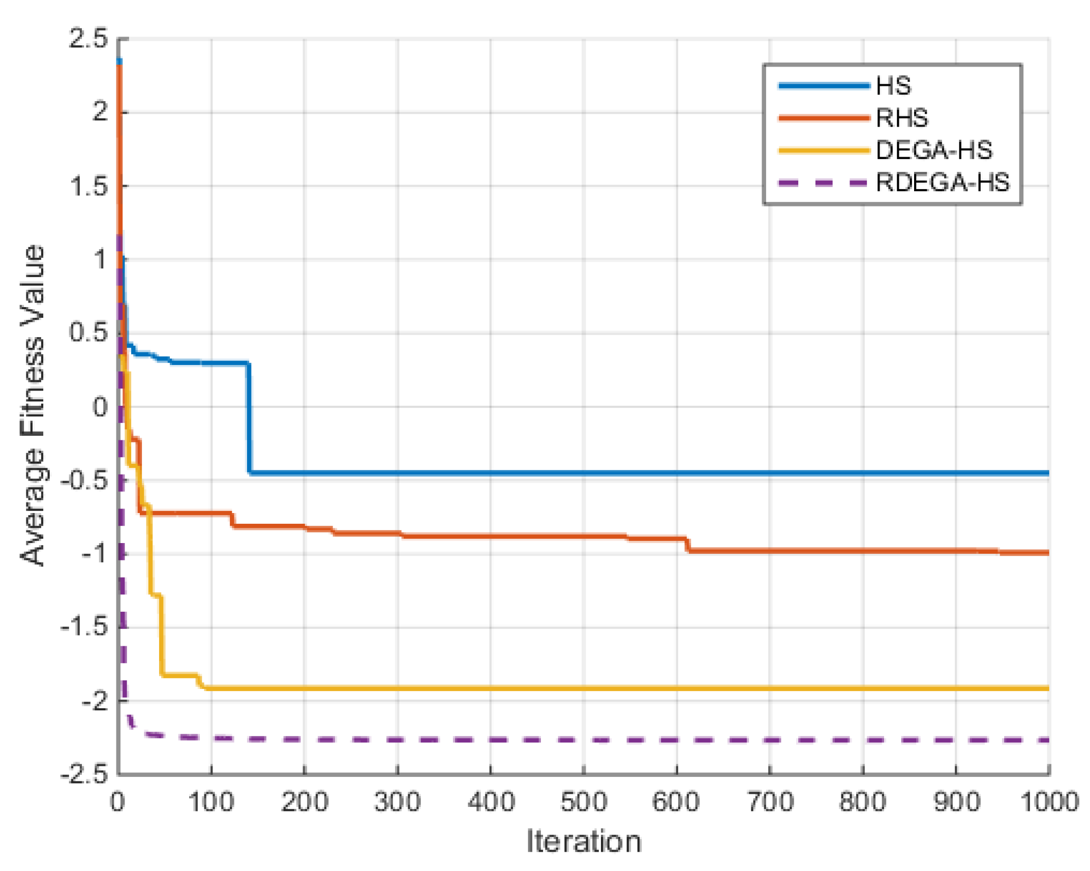
(1) Ackley Function
For the case where n = 40, the change in the average optimal fitness of the Ackley function with the number of iterations is shown in
Figure 4.
(2) Griewank Function
For the case where n = 40, the change in the average optimal fitness value of the Griewank function with the number of iterations in shown in
Figure 5.
(3) Rastrigin Function
For the case where n = 40, the change in the average optimal fitness value of the Rastrigin function with the number of iterations in shown in
Figure 6.
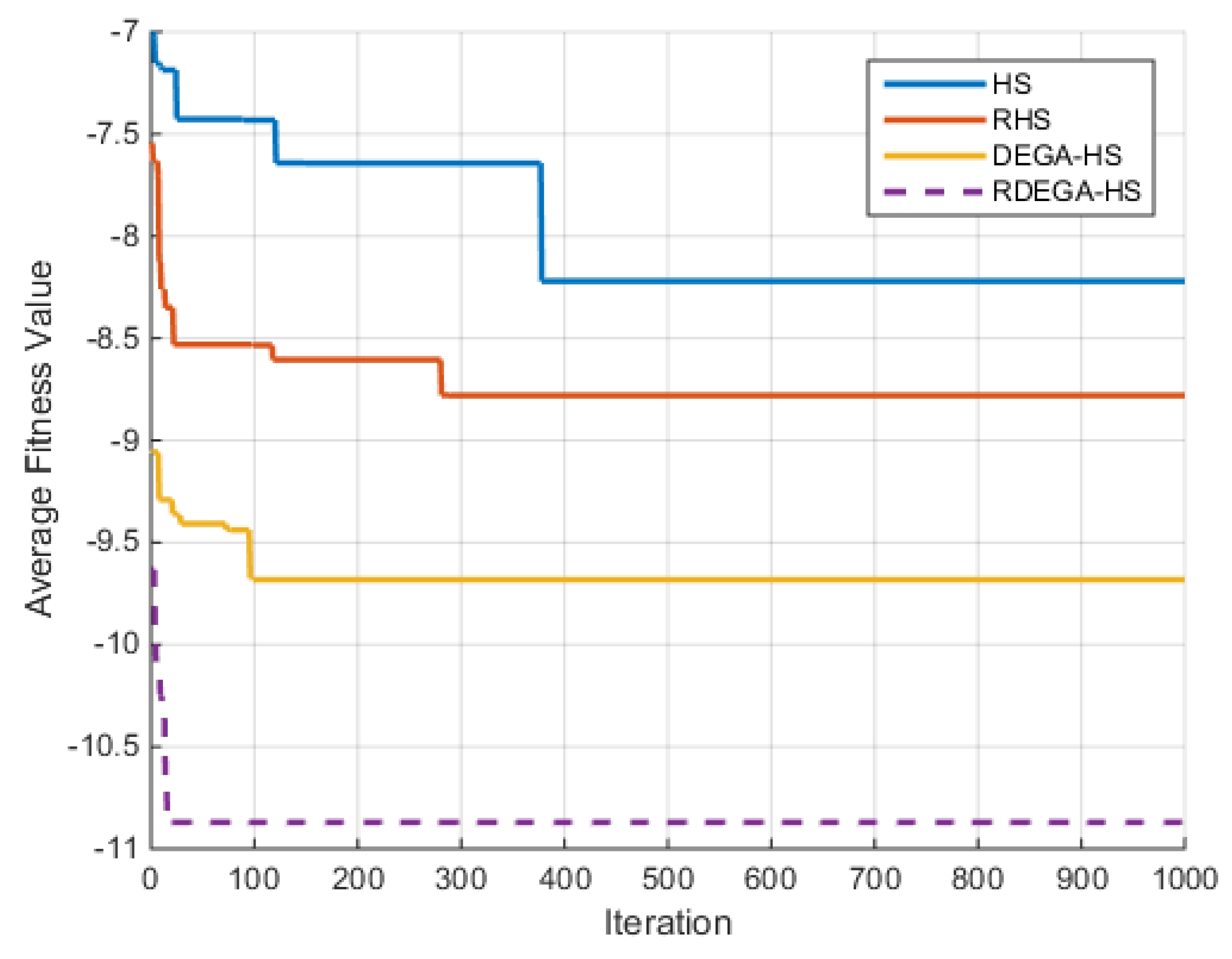
(4) Rosenbrock Function
For the case where
, the change in the average optimal fitness value of the Rosenbrock function with the number of iterations in shown in
Figure 7.
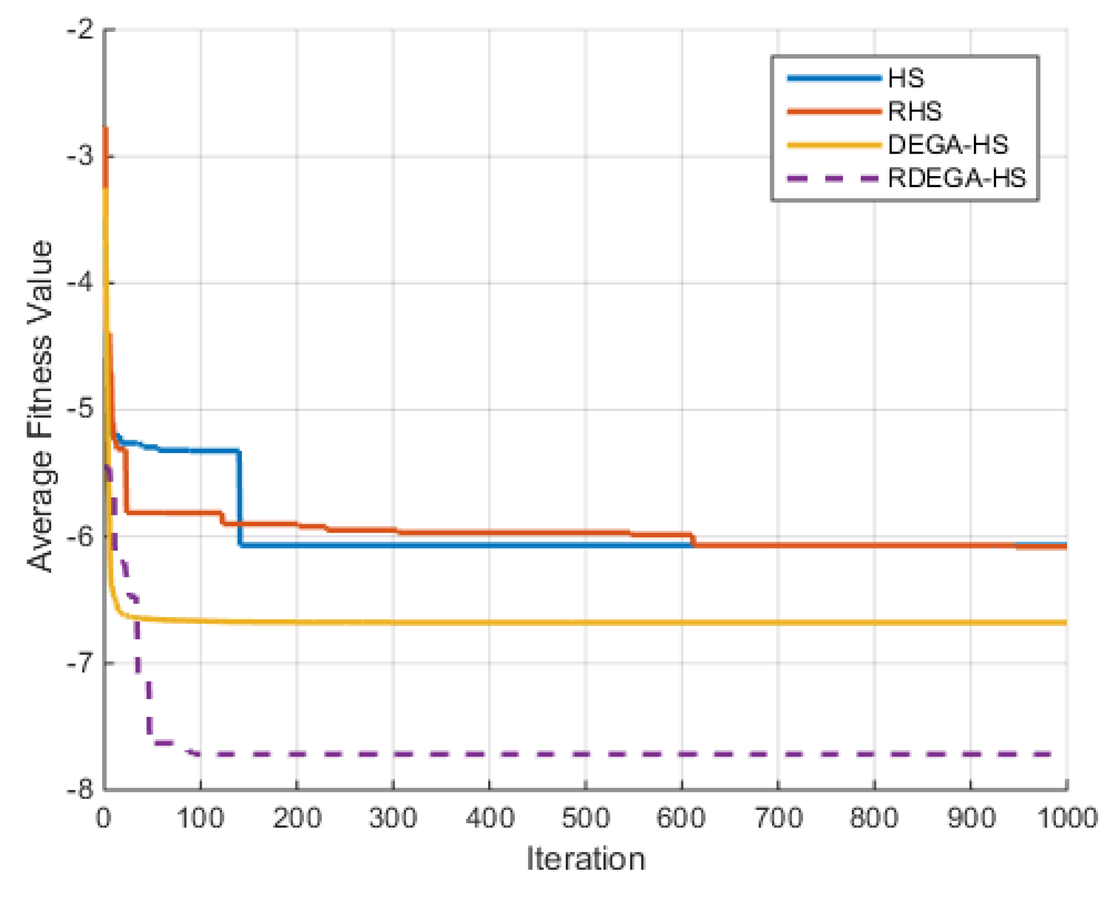
(5) Sphere Function
For the case where n = 40, the change in the average optimal fitness value of the Sphere function with the number of iterations in shown in
Figure 8.
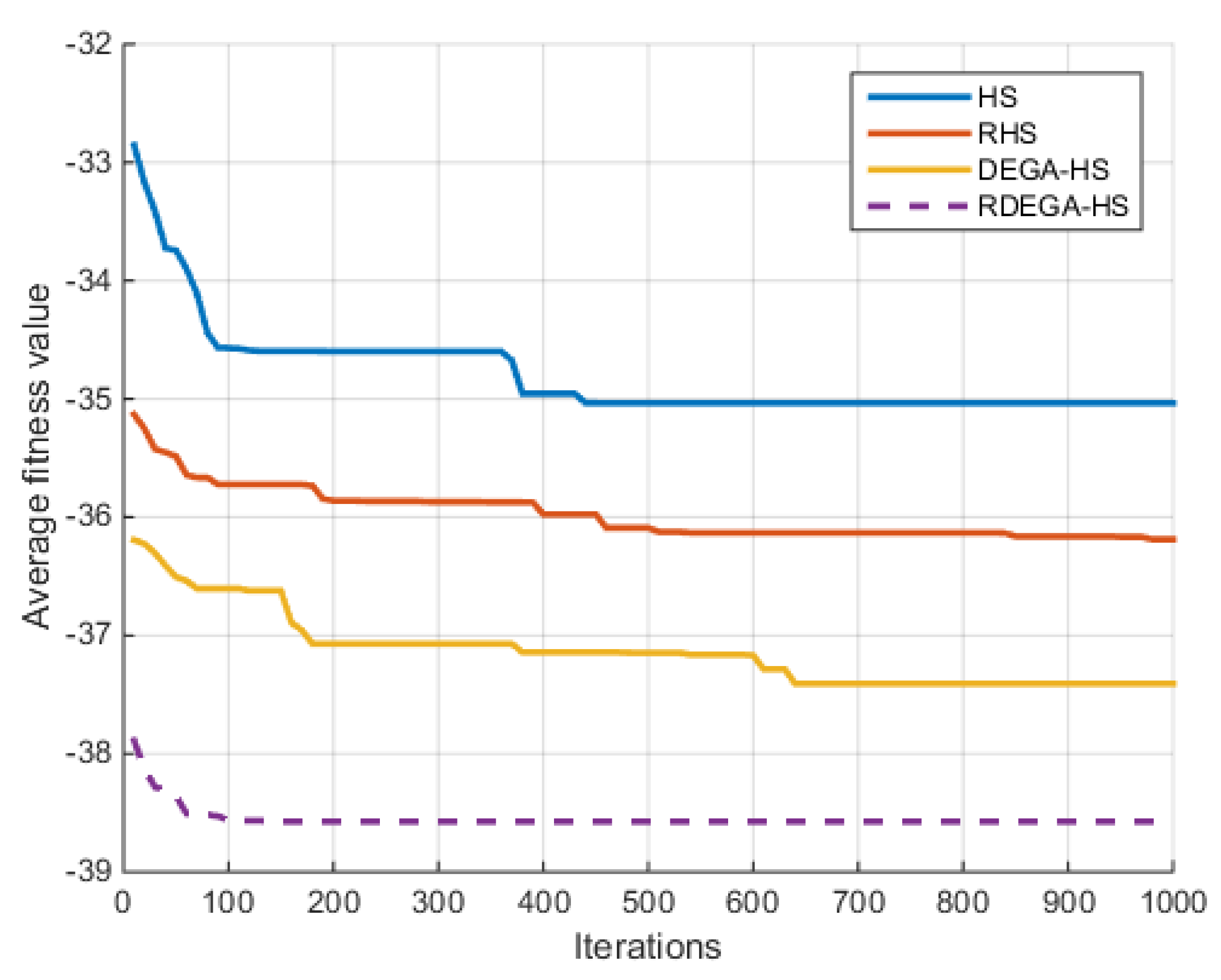
(6) Schwefel Function
For the case where n = 40, the change in the average optimal fitness value of the Schwefel function with the number of iterations in shown in
Figure 9.
It can be seen from the comparison of the optimization results of the test functions in
Table 4,
Table 5,
Table 6,
Table 7,
Table 8 and
Table 9 and the changes in average fitness in
Figure 4,
Figure 5,
Figure 6,
Figure 7,
Figure 8 and
Figure 9 that the proposed algorithm has a strong optimization ability. Upon a general review of each algorithm’s optimization process for the above six functions, the dimensions of the functions had a significant influence on the optimal value. As the dimensions increased, the optimal value of each algorithm also changed. For example, for the Ackley function, the variable dimensions had a significant influence on each algorithm. In terms of a low-dimensional function, RDEGA-HS and the other algorithms were all able to achieve the global optimum; however, in terms of a high-dimensional function, the RDEGA-HS algorithm still achieved a satisfactory result.
As to a comparison of the algorithms’ stability, the experiments were repeated 100 times. In addition to the optimization ability, which has received a lot of attention, the algorithms’ stability is also an index worth paying attention to when evaluating the performance of algorithms. After 100 repetitions, the variance in the experimental results was solved to check the fluctuation in the algorithms’ optimal value. For the six functions, the RDEGA-HS algorithm still maintained satisfactory stability, while the rest of the algorithms were quite unstable.
Since five sub-harmony memories have been designed and calculated for RDEGA-HS, the running duration is longer than an algorithm where a single-harmony memory is set. However, as the diversity of harmony memories is increased, the local optimal solutions are avoided, thus improving the solving accuracy.
5. Conclusions
In this paper, on the basis of the standard harmony search (HS) algorithm, a reward population mechanism, differential mutation, and Partheno-genetic operation were used to improve the basic harmony search algorithm, whereby the harmony vector diversity and accuracy were improved. With the introduction of the reward population mechanism, the harmony memory was divided into four common sub-harmony memories and one reward harmony memory, each of which adopts the evolution strategy of the differential genetic harmony search. After each iteration, the sub-harmony memory with the best optimal average fitness was combined with the reward harmony memory. The mutation strategy of the differential evolution (DE) algorithm is able to overcome premature convergence. By introducing the mutation strategy of DE into the HS algorithm, it was able to overcome premature convergence and improve the convergence rate. Meanwhile, the Partheno-genetic algorithm was introduced the generation of new harmony vectors. Finally, the six frequently used test functions of Ackley, Griewank, Rastrigin, Rosenbrock, Sphere, and Schwefel were introduced to verify the validity and convergence of the algorithms. Then, a comparison was made on the calculation results of the standard harmony search algorithm, reward population-based harmony search algorithm, differential genetic harmony search algorithm, and reward population-based differential genetic harmony search algorithm. The result suggests that the reward population-based differential genetic harmony search algorithm has advantages such as a strong global search ability, high solving accuracy, and satisfactory stability.


