Article

Parameter Optimization of Active Disturbance Rejection Controller Using Adaptive Differential Ant-Lion Optimizer

College of Information Science and Technology, Beijing University of Chemical Technology, Beijing 100020, China
*
Author to whom correspondence should be addressed.
Algorithms 2022, 15(1), 19; https://doi.org/10.3390/a15010019
Submission received: 27 November 2021 / Revised: 1 January 2022 / Accepted: 3 January 2022 / Published: 5 January 2022
(This article belongs to the Special Issue Bio-Inspired Algorithms)

Abstract

:
Parameter optimization in the field of control engineering has always been a research topic. This paper studies the parameter optimization of an active disturbance rejection controller. The parameter optimization problem in controller design can be summarized as a nonlinear optimization problem with constraints. It is often difficult and complicated to solve the problem directly, and meta-heuristic algorithms are suitable for this problem. As a relatively new method, the ant-lion optimization algorithm has attracted much attention and study. The contribution of this work is proposing an adaptive ant-lion algorithm, namely differential step-scaling ant-lion algorithm, to optimize parameters of the active disturbance rejection controller. Firstly, a differential evolution strategy is introduced to increase the diversity of the population and improve the global search ability of the algorithm. Then the step scaling method is adopted to ensure that the algorithm can obtain higher accuracy in a local search. Comparison with existing optimizers is conducted for different test functions with different qualities, the results show that the proposed algorithm has advantages in both accuracy and convergence speed. Simulations with different algorithms and different indexes are also carried out, the results show that the improved algorithm can search better parameters for the controllers.

1. Introduction

Active disturbance rejection control (ADRC) is a promising and relatively new control technology, which was formally proposed by Han in 2009 [1], while the origin of ADRC could date back to the year of 1995 [2]. Its core idea is to treat both internal uncertainty and external disturbance as “generalized interference”, estimate the generalized interference through a mechanism called “extended state observer (ESO)” in real time, and then compensate the generalized interference by a nonlinear feedback controller using the estimation of ESO. The greatest advantage of ADRC is that it only needs the relative order of the controlled object; thus, it is independent of a precise model of the controlled object. So far ADRC has been widely applied in many fields such as motion control [3], energy [4], chemical industry [5], power parafoil control [6], paper tension adjustment [7], and so on. ADRC has also shown broad commercial application value, one of the examples is InstaSPIN-MOTION motor control solution produced by Texas Instruments, which integrates ADRC inside to achieve high control performance.
Generally speaking, in the field of control engineering, how to obtain a set of controller parameters which can meet the specific performance index has always been a research topic. A set of optimized parameters can achieve better control performance, and this means a lot in industrial manufacturing, such as economic effects and even environment benefits. A properly designed and well-tuned ADRC can make the control system achieve good performance and robustness. However, in the design framework of origin ADRC, there are too many parameters that need to be adjusted, and the number of parameters will increase as the relative order of the controlled object increases. The number of parameters is one thing, the other complex thing is that these parameters interact with each other. Gao [8] proposed linear ADRC (LADRC) with scaling and a bandwidth parameterization method. The number of parameters of LADRC is successfully reduced to two, but the coupling effect between parameters still remains, and even becomes more obvious. Thus, it is rather difficult to analytically find the optimal parameters that can achieve good control performance. What’s more, if LADRC is applied on industrial processes with time delay, due to the existence of time delay, the characteristic function of system is a pseudo polynomial, which makes it even impossible to have an analytical solution. Although it is easy to find a set of parameters that make the control system stable, how to find the optimal system performance parameters has always been a problem demanding prompt study.
On the other hand, the process of finding optimal parameters of a control system can be regarded as an optimization problem with system performance index as the objective function [9]. Usually, the optimization problem designed by this method is a non-convex optimization problem, and it is difficult to solve by conventional optimization methods, which urges researchers to find a new way to solve this kind of optimization problem. In recent years, with the development of digital computers, more and more researchers turned their attention to meta-heuristic algorithms to solve engineering and practical problems. Türk, Deveci, et al. [10] used a simulated annealing algorithm to improve an interval type-2 fuzzy sets and achieved an outstanding result for an electric charging station location problem. Demirel and Deveci [11] successfully optimized medium-scale airline crew pairing problems by a modified genetic algorithm. Meta-heuristic algorithms benefit from the use of random operators [12]. Random operators make these algorithms exhibit completely different behaviors from deterministic algorithms and that is the reason why meta-heuristic algorithms usually have stronger global search ability.
The ant-lion optimization (ALO) algorithm is a relatively new meta-heuristic algorithm developed by Mirjalili in 2015 [13], which is also a kind of bionics algorithm. The ant-lion algorithm simulates the unique behavior of antlion in the process of hunting, which is to build a funnel-shaped trap and throw sand at the prey after the prey enters the trap to accelerate its slide to the bottom of the pit, as shown in Figure 1. The significance of imitating this behavior is to accelerate the convergence rate of the algorithm. In addition, the idea of elitism is also introduced into ant-lion algorithm. By setting an elite antlion to affect all ants, the convergence speed of the algorithm is accelerated.
In recent years, ALO has attracted the attention of researchers and proved its success in many applications including feature selection [14,15], multi-layer perceptron optimization [16], optimal reactive power distribution power system [17], optimal reactive dispatch problem [18], system identification [19], distributed generation planning [20], networking [21] etc. The references mentioned here all indicate that ALO has impressive characteristics including fast convergence speed, good solution quality, easy implementation and small quantity of parameters. Motivated by these facts, we propose a modified ALO, known as differential step-scaling ant-lion algorithm (DSALO), to optimize the parameters of LADRC. This algorithm can explore the search space efficiently and has a promising accuracy by global and local exploration. To our knowledge, ALO has not been adopted to solve the parameter optimization problem of ADRC, so this literature can be a worthwhile exploration.
The main contributions of this literature are as follows:
  • Differential evolution strategy is introduced into ALO to enhance the diversification of population in each iteration, which ensures the global exploration of the algorithm.
  • A step-scaling method is integrated into ALO, which changes the step size according to the number of iterations. The step-scaling method can achieve a good balance of exploration and exploitation.
  • DSALO algorithm is conducted on four representative test functions, compared with other algorithms to demonstrate its efficiency.
  • DSALO is applied in the parameter optimization problem of ADRC. The results indicate that DSALO can search for better parameters.
The remainder of this work is organized as follows. Section 2 presents the original ALO briefly and proposes DSALO. Section 3 evaluates the proposed algorithm by using 4 test functions. In Section 4, DSALO algorithm is used to solve the parameter optimization problem of the active disturbance rejection controller. Finally, some conclusions and future directions are drawn in Section 5.

2. Differential Step-Scaling Antlion Algorithm

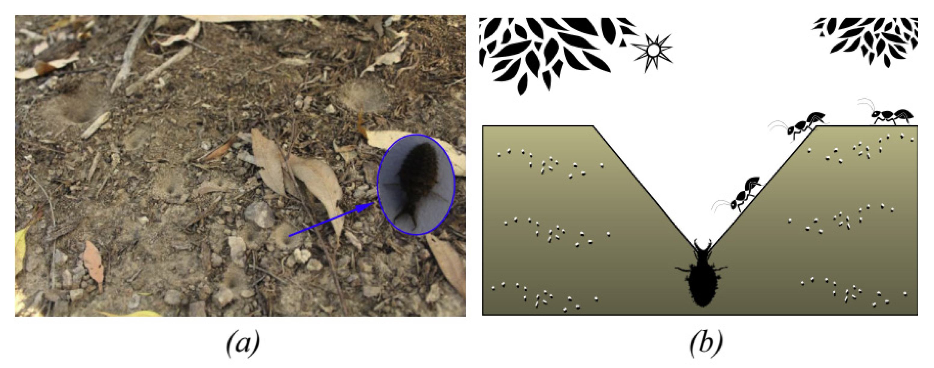
2.1. Antlion Algorithm

Ant-lion algorithm is a kind of meta-heuristic algorithm, which is inspired by the unique predation behavior of antlion, and it belongs to bionics algorithms. Antlions typically spend their larval years hunting and saving up energy, only reproducing as adults. As larvae, antlions use their jaws to dig a funnel-shaped sand pit and lie in wait for prey to appear. The edge of the pit is sharp enough to make it easy for the prey to fall into the pit. And when there’s prey, the antlion will try to catch it. But the prey will do anything to get out of the pit, and that’s where the antlion’s unique hunting behavior comes in: it moves towards the prey and throws sand at the prey, stopping it from escaping and speeding it down to the bottom of the pit. When they get close enough to capture their prey, the antlion drags it underground to digest it, then returns to the surface, where it dumps the residue while repairing its sandpit and waiting for the next victim to arrive. The probability of an antlion catching prey is related to the size of the pit, and studies have shown that the size of the pit is positively correlated with the degree of hunger of the antlion [22]. The hungrier the antlion is, the larger the pit it digs, then the greater the chance of catching prey it has, which is what antlions have evolved to ensure the survival of the colony.
The ant-lion optimization algorithm is inspired by the interaction between predator antlion and prey ant in the sand pit. In order to describe this interaction, we need to first model the ant’s walking route and the antlion’s predation and reconstruction behavior respectively. Since ants typically conduct a random walk when searching for food, they can be modeled using the following vector:
X ( t ) = [ 0 , c u m s u m ( 2 r ( t 1 ) 1 ) , c u m s u m ( 2 r ( t 2 ) 1 ) c u m s u m ( 2 r ( t m a x ) 1 ) ]
where, cumsum represents the sum of the past time of the random function r ( t ) , and tmax represents the maximum number of iterations. r ( t ) is a random function:
r ( t ) = { 1 r a n d > 0.5 0 r a n d 0.5
r a n d generates a random number evenly distributed between 0 and 1. Although the path of a single ant is random, reference [13] gives an example that this vector can ensure that the path of a colony of ants cover the entire search space.
It can be seen that for an individual ant, its walking route has already been determined when the algorithm is initialized. In addition, we need to define storage matrixes to store information about ants and antlions at each iteration:
M A = [ A 1 , 1 A 1 , 2 A 1 , d A 2 , 1 A n , 1 A n , d ]
M A L = [ A L 1 , 1 A L 1 , 2 A L 1 , d A L 2 , 1 A L n , 1 A L n , d ]
where Ai,j represents the j-th dimension information of the i-th ant and A L i , j the corresponding information of the antlion. Each row in the two matrices represents a solution to the problem to be optimized. Moreover, we can define the position information of each ant and antlion as:
P A , i ( t ) = [ A i , 1 , A i , 2 , , A i , d ]
P A L , i ( t ) = [ A L i , 1 , A L i , 2 , , A L i , d ]
To evaluate the value of each solution, we need to calculate their fitness functions one by one and store the values of fitness functions in the following two matrices:
M O A = [ f ( A 1 , 1 , A 1 , 2 , , A 1 , d ) f ( A 2 , 1 , A 2 , 2 , , A 2 , d ) f ( A n , 1 , A n , 2 , , A n , d ) ]
M OAL = [ f ( A L 1 , 1 , A L 1 , 2 , , A L 1 , d ) f ( A L 2 , 1 , A L 2 , 2 , , A L 2 , d ) f ( A L n , 1 , A L n , 2 , , A L n , d ) ]
Thus, we can summarize the overall steps of the antlion algorithm:
The first step is the random walk of ants. All ants carry out the random walk according to Equation (1) and ensure that every dimension of ants carry out the random walk. In order to ensure that all ants are in the search space, the following formula is used to normalize the position of ants:
P A , n d ( t ) = ( P A , n d ( t ) m i n R ( P A , n d ) ) ( U d ( t ) L d ( t ) ) max R ( P A , n d ) min R ( P A , n d ) + L d ( t )
where P A , n d ( t ) is defined as the d-th ant variable in the t-th iteration, m a x P ( S A , n d ) and m i n P ( S A , n d ) represent the maximum and minimum value of the ant in the dimension respectively, U d ( t ) and L d ( t ) are the upper and lower limit of the dimension d in the t-th iteration.
The second step is to simulate the process of ants being trapped in the sand pit. In reality, the actions of ants will be affected by antlions. Therefore, in order to simulate this process, we need to use the following two expressions to update the upper and lower bounds of ants’ random walk:
U t d ( t ) = { P A L d ( t ) + U t d     if   rand > 0.5 P A L d ( t ) U t d           otherwise      
L t d ( t ) = { P A L d ( t ) + L t d     if   rand > 0.5 P A L d ( t ) L t d           otherwise
The third step is to simulate the antlion’s trap-building process. To achieve this, a strategy called roulette wheel is introduced into the antlion algorithm. In the ant-lion algorithm, one ant can only correspond to one antlion, so roulette wheel strategy is used to determine which ant it can capture according to the fitness value of the antlion. This strategy has a high probability that a better-fit antlion will capture a better-fit ant.
The fourth step is to simulate the process of an antlion throwing sand to make its prey slide to the bottom of the pit. In the algorithm, we assume that antlions with better fitness build bigger traps. Although the ant is random, when it gets close to the antlion, the antlion throws sand at it and thus it slides to the bottom of the pit. From the perspective of mathematical model, it can be understood that the range of the ants’ movements is getting smaller and smaller. Therefore, the algorithm uses the following conditions to update the upper and lower bounds of the ants’ migration:
L d ( t ) = L d ( t ) I
U d ( t ) = U d ( t ) I
In Equations (12) and (13), the value of I is defined as I = 10 w t c u r r e n t / t m a x , where t c u r r e n t is the current iteration number, t m a x is the maximum iteration number, and w is a value determined according to the current iteration number ( t c u r r e n t > 0.1 t m a x then w = 2 , t c u r r e n t > 0.5 t m a x then w = 3 , t c u r r e n t > 0.7 t m a x then w = 4 , t c u r r e n t > 0.9 t m a x then w = 5 , t c u r r e n t > 0.95 t m a x then w = 6 ). By changing the value of w during different iterations, the accuracy of the algorithm search can be adjusted.
The fifth step is to simulate the process of the antlion capturing prey and rebuilding the trap. When the ant finally falls into the antlion’s mouth and is captured by the antlion, the antlion burrows underground in its current position to digest the ant, and after digesting the antlion returns to the surface to reconstruct the trap. In the algorithm, this process is the updating of the fitness value of the antlion. Assuming that the antlion will only capture the ants with better fitness than itself, the position of the antlion after the capture is the same as that of the ant before. This process can be simulated by the following formula:
P A L , j ( t ) = P A , i ( t ) , i f f ( P A , i ( t ) ) < f ( P A L , j ( t ) )
where P A L , j ( t ) is the position of the j-th antlion at t-th iteration, and P A , i ( t ) is the position of the i-th ant at t-th iteration. To achieve this behavior, it is needed to rank all f ( P A L , j ( t ) ) and f ( P A , i ( t ) ) in ascending order of their numeric value, then update the first N lines of f ( P A L , j ( t ) ) to f ( P A , i ( t ) ) , and update the corresponding position information P A L , j ( t ) at the same time.
Finally, elitism is introduced into ant-lion algorithm. Elitism is an important feature of evolutionary algorithms, enabling them to maintain the best solution obtained at any stage of the optimization process. In ALO, the best antlions obtained so far in each iteration are saved and considered elite. Since elite is the most adaptable antlion, it should be able to influence the movement of all ants during the iteration. Therefore, the algorithm assumes that each ant simultaneously walks randomly around the selected colony via roulette wheel and elite, as shown below:
P ( A , n ) d ( t ) = R A ( t ) + R E ( t ) 2

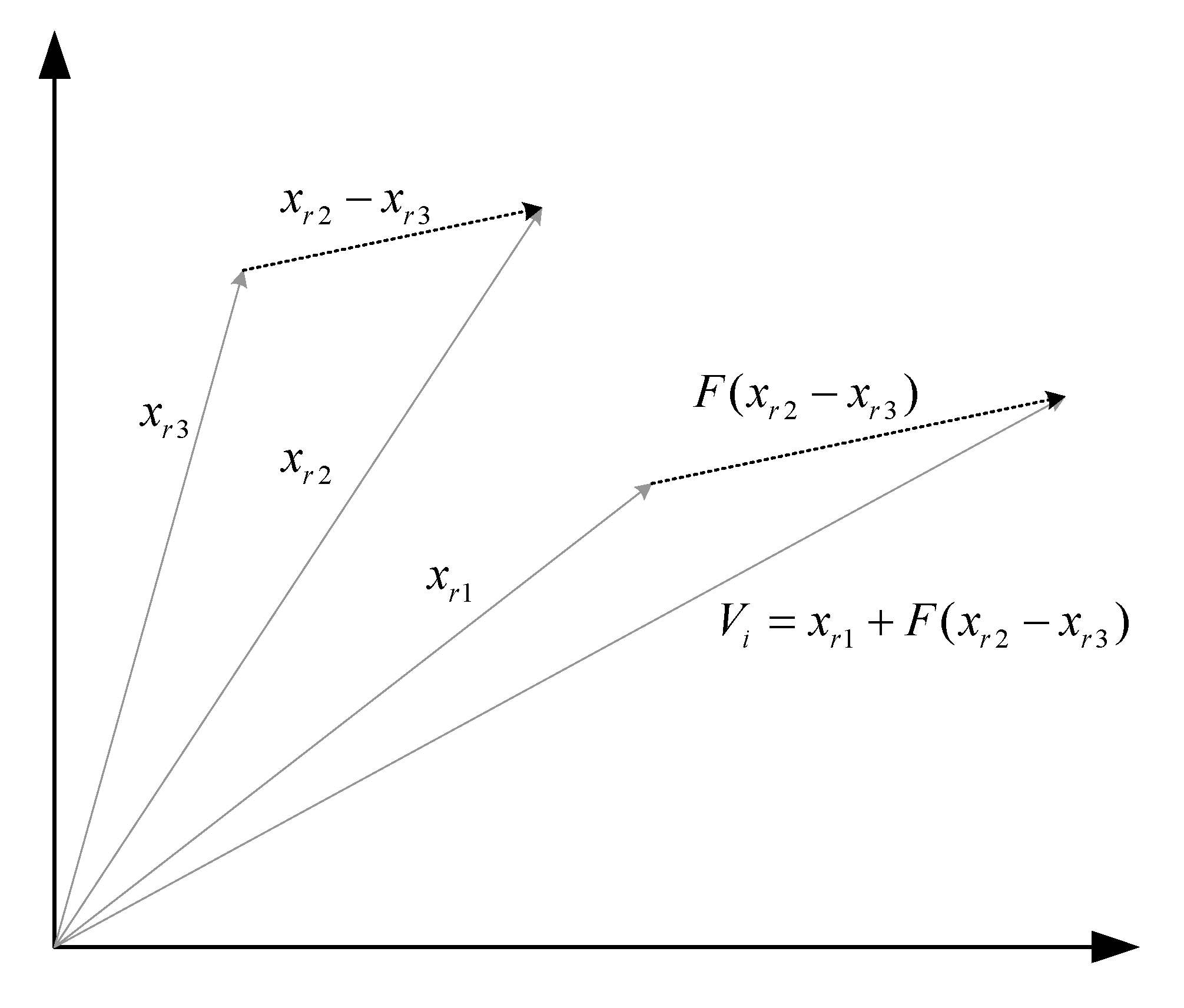
2.2. Differential Step-Scaling Ant-Lion Algorithm

For a meta-heuristic algorithm based on swarm agents, the migration strategy of the agent has a crucial influence on the convergence, stability, and speed. The same is true for ant-lion algorithms. Although each ant walks randomly when the algorithm is initialized, with the increase of iterations, we can know that better fitness values cannot be obtained in some search domains, so gradually there is no need to let the random walk of ants fill the whole space. In other words, in some other areas, we need to pay more attention, because the near-optimal solution (an accepted common sense is that intelligent optimization algorithms cannot really achieve the global optimization of the problem but can only obtain a near-optimal solution in an infinitesimal neighborhood of the global optimization. But when the error is small enough, we can assume that the result returned by the algorithm is globally optimal) is probably in one of these regions. That is also the reason that the idea of elitism and boundary reduction is introduced in ant-lion algorithm.
However, although in the telocinesia of iterative we don’t need to let the search bodies traverse the entire space, at the beginning of the iteration, the range that search bodies can reach is still the bigger the better. Although the introduction of elitism can guarantee strong searching ability near global optimal solution in the later period of iteration, it can be seen from the Equation (15) that in the iterative process of the ant-lion algorithm, the attraction of elite antlion to all ants is fixed, which weakens the initial global search ability of the algorithm. Therefore, this paper introduces the idea of step scaling. The change in “step size” here is not the step size of each ant as it migrates, but the change in the influence of the elite antlion on the entire ant population in each iteration. At the beginning of the algorithm, the influence of the elite antlion is loosened so that the ants can explore the whole parameter space more “freely”. At the end of the algorithm, the influence of the elite antlion is restored to its original state, which ensures that the improved algorithm has the same global optimal searching ability as the original antlion algorithm. Therefore, P ( A , n ) d ( t ) is redefined as:
P ( A , n ) d ( t ) = R A ( t ) + R E ( t ) 2 × sin ( current maxgen × π 2 )
where R A ( t ) is the random walk around ants S s e l , R E ( t ) is the random walk around the elite antlion S e l i t e , current is the current iteration number, and maxgen is the maximum iteration number set.
The reason for choosing a sine trigonometric function as multiplier in Equation (16) is that although we need to enhance the wandering ability of search bodies in the early stage of the algorithm, we don’t need to let them “indulge” for too long. The sinusoidal trigonometric function has a high rising speed in the initial stage and will change rapidly with the change of the independent variable, thus playing a role of scaling step size, and the whole scaling process is smooth.
In addition, in order to enrich the population diversity and further increase the global searching ability of the ant-lion algorithm, a method that can enhance the global searching ability of the ant-lion algorithm should be introduced. A differential evolution algorithm is a reasonable solution. The algorithm was originally proposed by Storn and Price on the basis of the evolutionary idea of a genetic algorithm [23]. It is essentially a multi-objective continuous variable optimization method, used to solve the global optimal solution in multi-dimensional space. Compared with a genetic algorithm, their common point is to randomly generate the initial population, respectively calculate the fitness value of each individual in the population and select individuals according to the value of fitness. Their main processes both include mutation, crossover, and selection. The difference is that a genetic algorithm uses the fitness value of individual population to control the parent population for hybridization, and then carries out a mutation operation to obtain the probability value of offspring being selected. In a differential evolution algorithm, each individual in the population is regarded as a vector. Through vector calculation, the parent vector is calculated by difference to generate a mutation vector, and then the mutation vector is hybridized with the parent vector to generate a new vector, which is regarded as the child and selected with the parent directly, as shown in Figure 2. Differential evolution algorithms have strong robustness, fast convergence speed, and the most important thing is that they are easy to implement. The calculation steps of a differential evolution algorithm mainly include three stages: mutation, crossover, and selection, and “DE/x/y/z” is usually used to distinguish and represent different evolution methods and operators. In “DE/x/y/z”, x specifies how to choose a basis vector; y specifies the number of difference vectors in evolution; z is a way of crossing operations. In addition to selecting strategies for specific problems, the performance of a differential evolution algorithm is also related to three key parameters: population size NP, scaling factor F, and crossover probability CR. A reasonable evolutionary strategy and a set of appropriate key parameters can greatly improve the convergence speed and accuracy of the algorithm.
In this paper, we choose the “DE/rand/1/binDE” mode, initialize all the individuals of the population into n-dimensional vectors, and then randomly generate individual positions in the search area. In the mutation stage, two vectors are randomly selected for difference operation to obtain the mutation vector, and then the mutation vector is scaled and added with a third parent vector to obtain a new child vector. The binomial crossover operator was used to ensure that at least one dimension of the final test individual comes from the mutant individual, so as to avoid being the same as the current individual and ensure the diversity of the population. A random number conforming to uniform 0–1 distribution is generated and compared value with the crossover probability CR. If the value of the random number is less than CR, the value of the mutant individual at this dimension is given to the test individual, or the value of the test individual at this dimension will come from the current individual. In the selection stage, the fitness values of the new individuals and the original individuals after mutation and crossover are compared, and the excellent ones are retained while the bad ones are discarded to ensure that the individuals in the population are currently optimal before entering the next iteration.
Specifically in this paper, the combination points of the differential evolution algorithm and the ant-lion algorithm are as follows:
In each iteration, after obtaining all antlions at the current iteration, the antlions were variated and differentiated.
Mutation: select several pairs of antlions randomly, regard them as the parent vector, calculate the difference between them and scale them according to the scaling factor, then add the scaled difference vector and the vector of the third antlion individual to obtain a new test body, the formula is defined as follows:
P ( t ) = P A L , r 1 d ( t ) + F ( P A L , r 2 d ( t ) P A L , r 3 d ( t ) )
where F is the scaling factor, r 1 , r 2 , r 3 is the three different random numbers in the interval [1, N], P ( t ) is the test object obtained by mutation operation in the t-th iteration, and P A L , r 1 d ( t ) , P A L , r 2 d ( t ) , P A L , r 3 d ( t ) is r 1 -th, r 2 -th, r 3 -th antlion vector of this iteration. After that, in order not to make the test body run out of the search range, boundary condition judgment is also needed, and the formula is as follows:
P = { L d ( t ) , i f S < L d ( t ) U d ( t ) , i f S U d ( t )
where S are the individual positions of antlions after mutation, L d ( t ) and U d ( t ) are the upper and lower bounds of all ants and antlions in the d-th dimension at t-th iteration.
Crossover: firstly, the crossover probability CR is determined, and the crossover operator is generated. In this work, we select the binomial operator to randomly generate a dimension identifier, then generate a random number with uniform distribution within the interval [0, 1], and compare its value with CR. Thus, a better individual can be selected:
U i = { P , if r 4 C R P , otherwise
where r 4 [ 0 ,   1 ] is a uniformly distributed random number, CR is crossover probability, also generated between 0 and 1; P is a mutant, P E is the elite antlion, U i is a new individual retained from the crossover.
Selection: compare the fitness values of the elite antlion PE with the fitness values of Ui in the previous step, discard those that do not meet the optimization requirements, and retain the better ones. The formula is as follows:
P A L = { U i , if f ( U i ) f ( P E ) P E , otherwise
In this way, the population diversity of elite antlions is enriched, and the remaining antlion population is not weaker than the original antlion population, which further improves the searching ability of antlion algorithm.

2.3. Algorithm Idea and Specific Steps

The improvement of the algorithm mainly focuses on the enrichment of population diversity and improvement of local search ability. The pseudo-code corresponding to the Algorithm 1 is shown as follows:
Algorithm 1 Pseudo-Code of DSALO
Initialize the first population of ants and antlions randomly
Calculate the fitness of ants and antlions
Find the best ant or antlions, then set it as the initial elite antlion
While the maxmum iteration is not reached
For each ant
 Select an antlion using Roulette wheel
 Update boundaries using Equations (12) and (13)
 Make a random walk using Equation (1)
 Normalize and update the position of ant using Equations (9) and (16)
End for
 Calculate the fitness of all ants
 Replace an antlion if its corresponding ant becomes fitter
 Apply Mutation, Crossover, and Selection operator to antlions
 Update the elite antlion
End while
Return the elite antlion

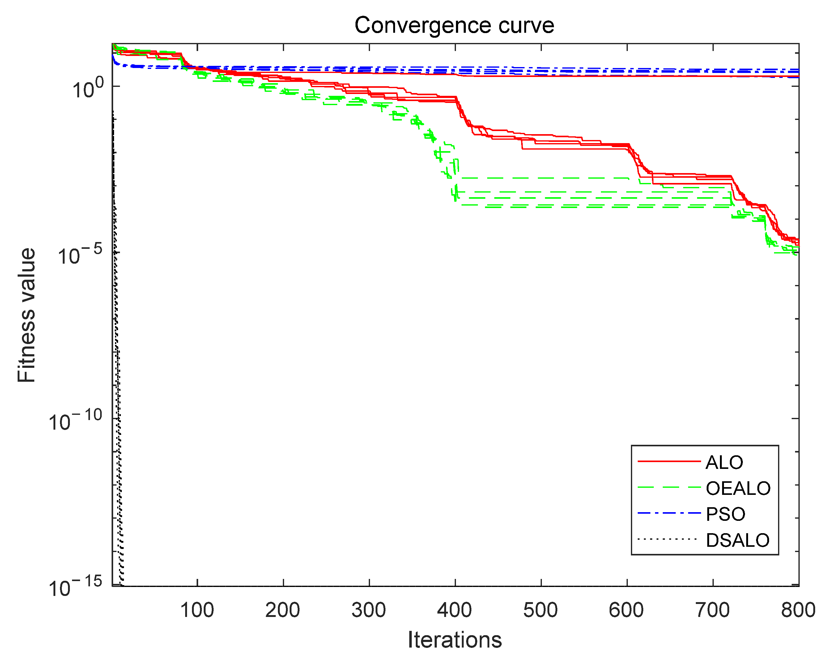
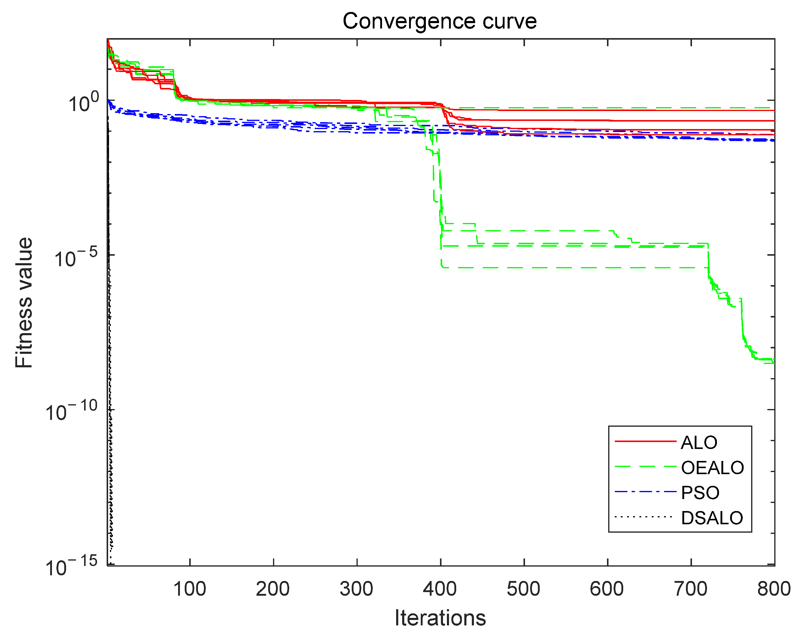
3. Performance Evaluation of Differential Step-Scaling Ant-Lion Algorithm

3.1. Algorithm Evaluation Criteria

When we use a test function, the optimal value of each test function is already known. Because of the random walk strategy of the algorithm, the results of the algorithm in each run may be different. Considering the stability and accuracy of the algorithm, the mean value of fitness, standard deviation, maximum and minimum are selected as evaluation criteria of the algorithm.
For an algorithm, if it can obtain a fitter mean value closer to the optimal value, a smaller fitness standard deviation, a smaller fitness maximum value as well as a smaller fitness minimum value, it indicates that the algorithm is excellent, or better than other algorithms in the problems applied in this comparison.

3.2. Test Function

The test functions, corresponding solution intervals and optimal values used in this paper are shown in Table 1. Of the four test functions, F1 is a unimodal function, F2 and F3 are multimodal functions, and F4 is a composite function [13].

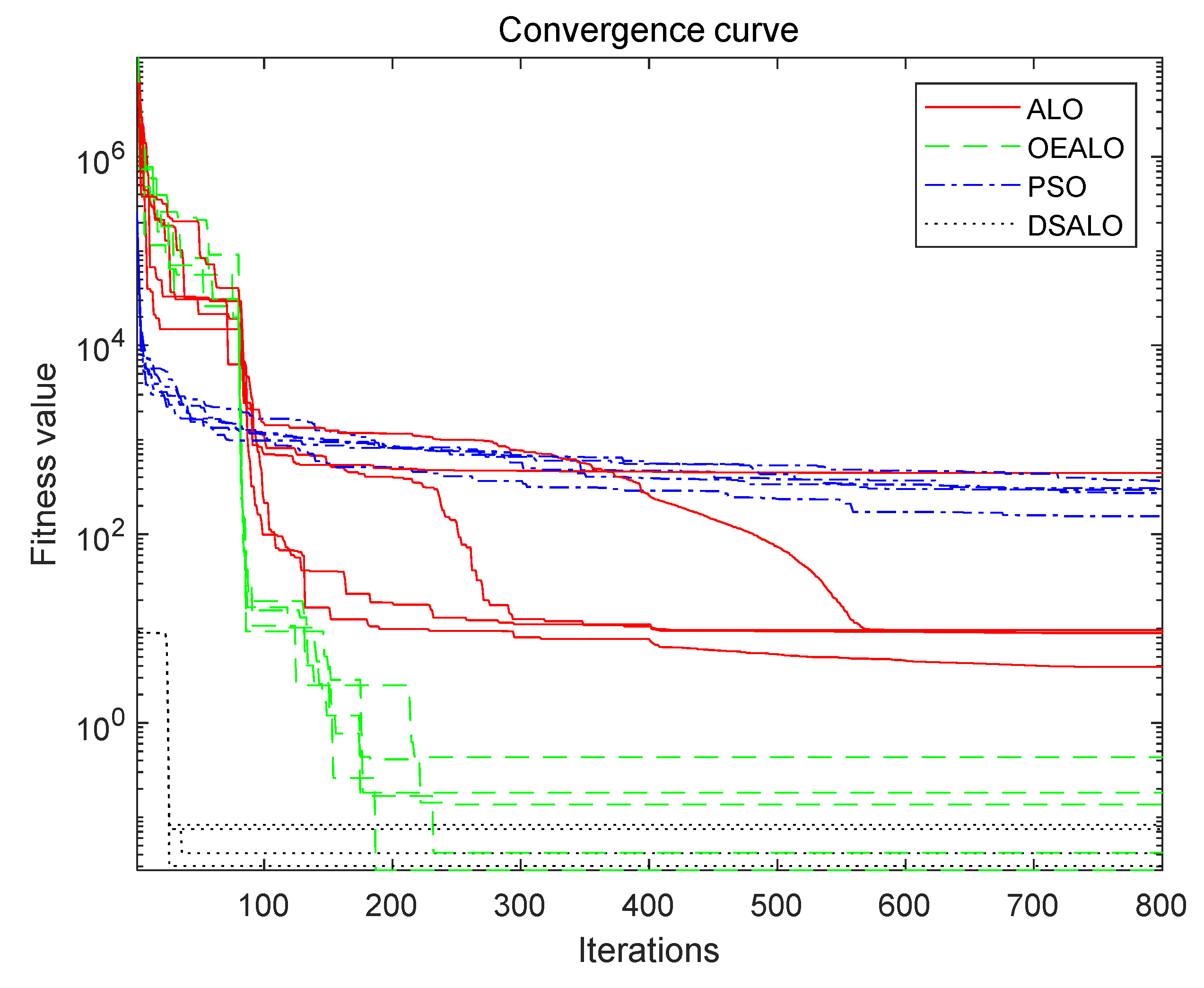
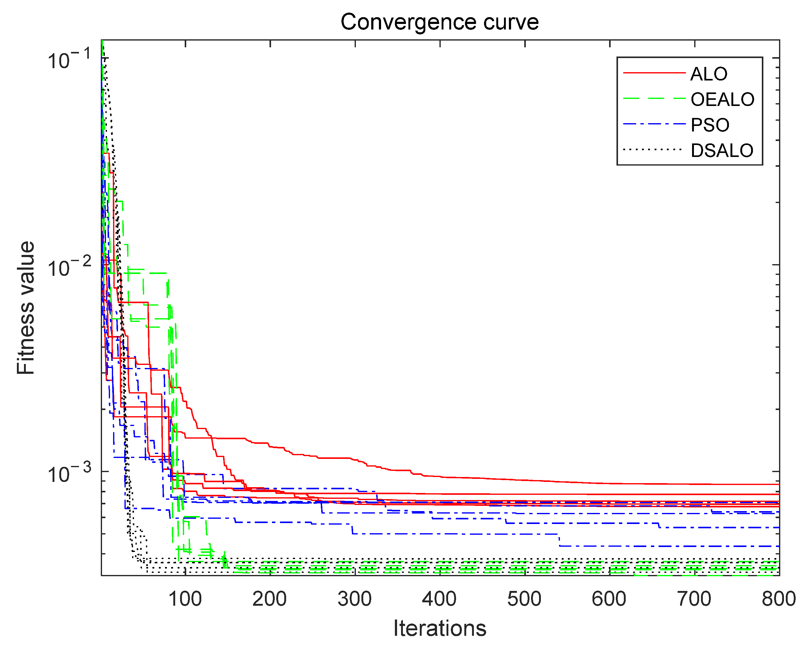
3.3. Analysis of Test Results

In this paper, DSALO is compared with ALO, PSO, and OEALO (Opposition based Exploratory differential Lion-based Optimization [24]). The dimension of test functions is set to 50. The test results are shown in Table 2. It can be seen from the table that DSALO has significantly improved the search accuracy, which indicates that DSALO has some certain advantages. Since the original ant-lion algorithm randomly selects the initial value when the algorithm starts to run, the dependence of the ant-lion algorithm on the initial value is low, while the DSALO algorithm inherits this characteristic of the original ant-lion algorithm.
The DSALO algorithm not only improves the accuracy, but also improves the convergence speed and stability. To intuitively demonstrate this point, the convergence curves of the DSALO algorithm, original ALO algorithm, PSO algorithm, and OEALO algorithm with 5 times of running on test functions F1 to F4 are shown in Figure 3, Figure 4, Figure 5 and Figure 6 respectively. The test functions are all set as 100 dimensions and the maximum iteration is set to 800. It can be seen that, on the test function F1, the DSALO proposed in this paper has a relatively strong improvement in both convergence speed and accuracy. On the test function F2, the PSO algorithm falls into local optimum earlier. ALO can avoid falling into local optimum, but its optimization accuracy is not as good as DSALO. OEALO’s effect is better than ALO but still has a disparity with DSALO. On the test function F3, both PSO and ALO fall into local optimum earlier. On the test function F4, DSALO and OEALO have similar performances and both of them are better than PSO and the origin ALO. From these results it can be concluded that DSALO has a significant performance improvement for multimodal functions, and has a similar performance with OEALO for unimodal and composite functions. Although DSALO has a similar effect to OEALO, it has a faster convergence speed. Since the four test functions in this section belong to different types of functions, so it can be shown that the DSALO algorithm has performs well in unimodal functions, multimodal functions, and composite functions.

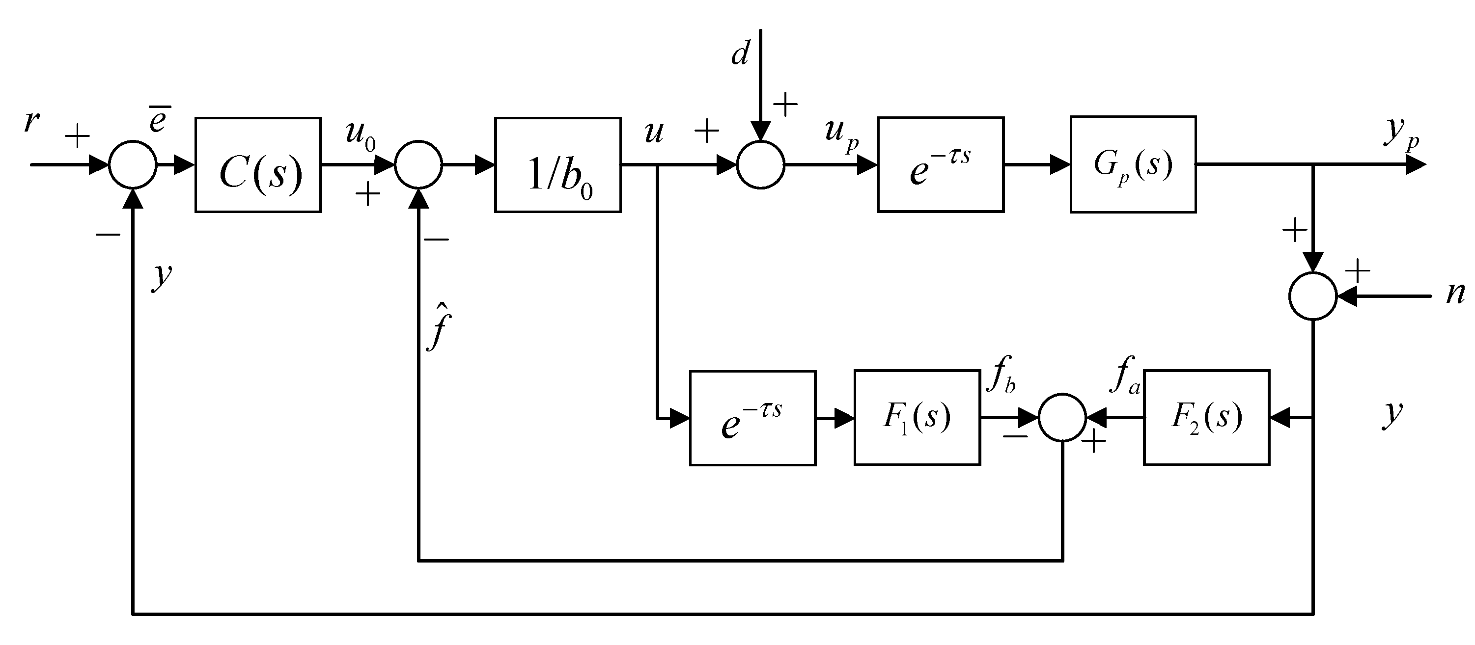
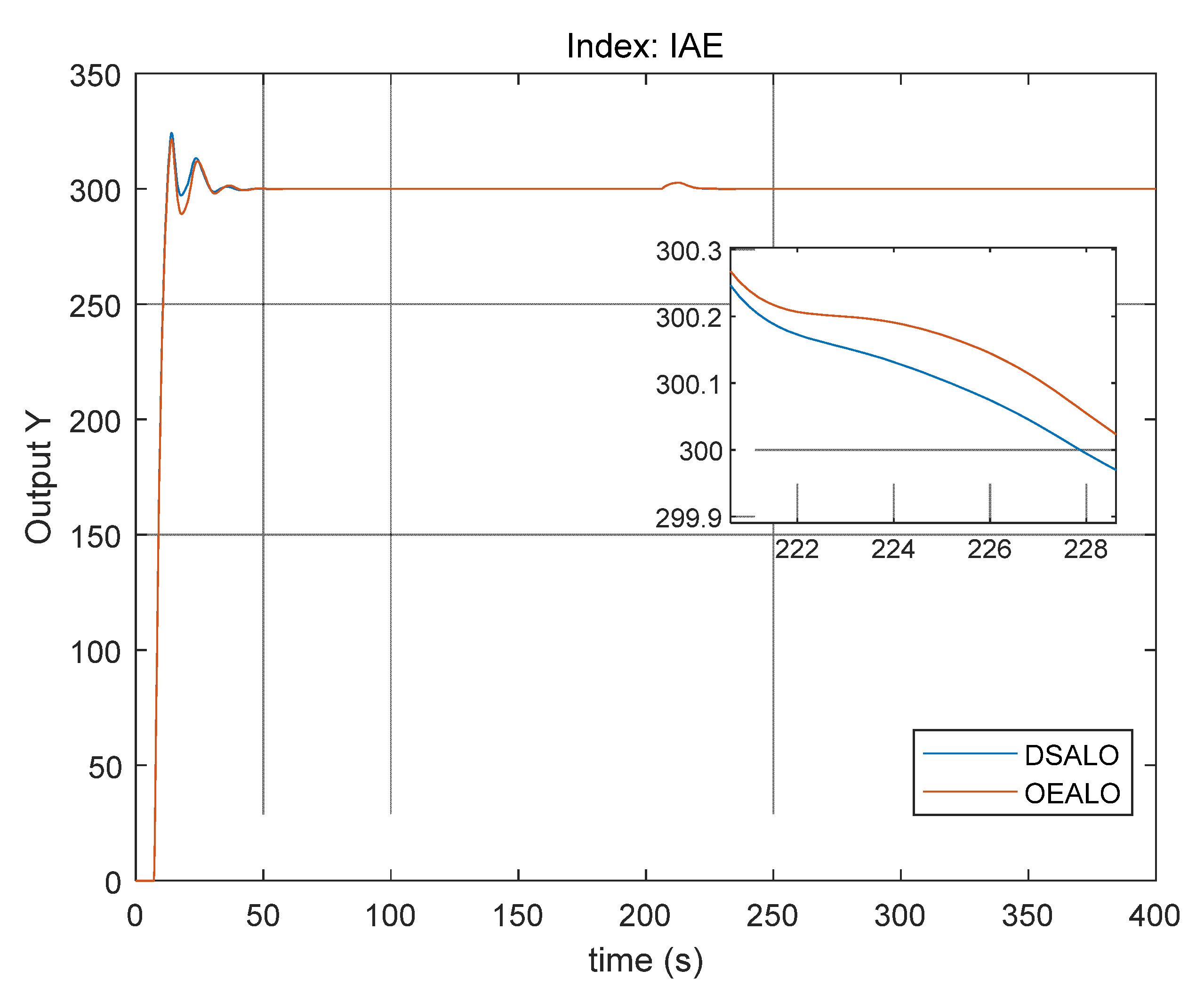
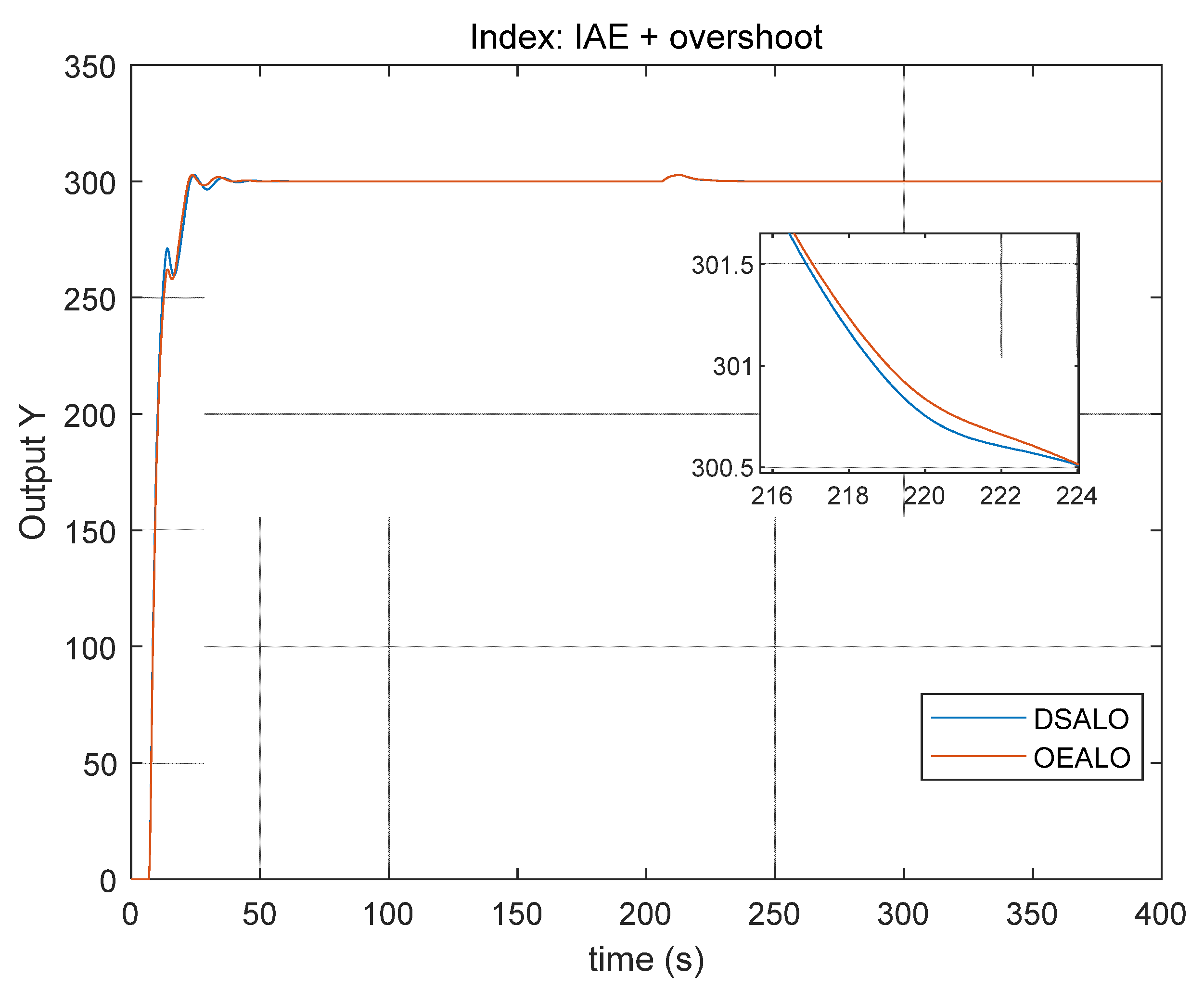
4. Parameter Optimization of ADRC

In this section, the effectiveness of the DSALO algorithm is illustrated by examples. The controlled object is assumed to be a tank in industrial manufacture. In the parameter optimization problem of a linear active disturbance rejection controller, the structure used is shown in Figure 7:
The controlled plant is a second-order system with time delay:
G p ( s ) = e 6 s s 2 + 3 s + 1
The observer is designed as
F 1 = ω o 2 ( s + ω o ) 2 , F 2 = ω o 2 s 2 ( s + ω o ) 2
The controller takes the proportional controller ω c .
Thus, we obtain a parameter set { ω o , ω c } to be optimized.
There are two parameters optimization objectives: one is to minimize the IAE index of the system; the other is to reduce the overshoot of the system as much as possible while considering the IAE index. Since in this paper the performance of DSALO and OEALO has been verified in Section 3 that they are both better than the original ALO and PSO, only DSLAO and OEALO are considered for comparison in this section. Given the randomness of the algorithms, each algorithm is run 25 times, and only the best results are recorded.
The authors run the simulation of ADRC parameters optimization in the following hardware environment: Intel® Core™ I7-8700K, Nvidia GeForce GTX 1060, and 16GB memory. The software environment is a Windows 10 operating system and Matlab R2020b. According to statistics, when the number of populations is set to 50 and the algorithm iterates 100 times, the average time of running DSALO to optimize the active disturbance rejection controller is 32 min, and the average time of running OEALO is 34 min. Given the complexity of the algorithm and the long control cycle in the process industry, such operation time is acceptable. It is worth noting that due to the existence of uncertainty, parameter optimization usually needs to be run at regular intervals. A large number of iterations can obtain better parameters but is also time-consuming, which may lead to a phenomenon that the optimization time takes up too much ratio of running interval or even is longer than the running interval. This phenomenon may cause parameter updates to be delayed, which in turn has a negative impact on the effectiveness of control. So, in the problem of ADRC parameter optimization, it needs a compromise between the optimization effect and computation time. That is the reason why we choose to set the number of iterations to 100.
The search results of parameters under the two targets are listed in Table 3. Figure 8 and Figure 9 show the corresponding output.
There is also one thing worth noting. The DSALO algorithm can be applied in industrial ADRC systems in this way: first collect input and output data of controlled plant to establish current model of the plant, then integrate the model in simulation software and take the control performance as objective function/fitness, finally run the simulation and DSALO simultaneously and the solutions of DSALO are the optimized parameters of ADRC.
It can be seen from the diagram, whichever kind of index or which kinds of optimization algorithm are used, the optimized performances of disturbance rejection (200 to 250 s) are very good. The difference mainly exists in the procedure of setpoint tracking (0 to 50 s). Using the parameters obtained by the DASLO algorithm can obtain smaller indexes. Combined with the meaning of IAE index, which is the corresponding energy consumption (coal, fuel, natural gas, etc.), the parameters obtained by DSALO have smaller performance metrics, which means better economy of the optimized system and better for the environment.

5. Conclusions and Future Perspectives

In this paper, an improved ant-lion algorithm called DSALO is proposed to solve the parameter optimization problem of ADRC. Because parameters of ADRC are directly related to the control performance, ulteriorly the economic effectiveness of the controlled object, finding an optimized set of parameters is of great importance. Specific to this work, a parameter set { ω o , ω c } is optimized with two performance indexes: IAE and IAE + overshoot. These indexes are important because they can reflect the economic effectiveness of a controlled plant in industrial manufacturing. In order to improve search abilities of origin ALO, differential evolution strategy is introduced to improve global search ability and a step scaling method is used to enhance local search ability. Experiments on test functions show that the DSALO algorithm has a significant improvement in accuracy for multimodal functions and a significantly higher convergence speed for unimodal functions, multimodal functions, and composite functions. The experimental results show that the DSALO algorithm has a batter optimization effect, further show that DSALO is capable of an ADRC parameter optimization problem. Since this is the first time using an ant-lion based algorithm to optimize the ADRC parameter, this study can be a basis of future optimization work for different ADRC varieties and nonlinear ADRC.
It should be noted that, however, some aspects can be studied in future work. One aspect is that DSALO does not show significant accuracy improvement, though a small improvement exists, for unimodal functions and composite functions. This phenomenon needs more study and DSALO may need modification at a deeper level. On the other hand, the convergence speed of DSALO still needs further improvement. As stated in this paper, an industrial application of optimization algorithms usually inherently compromises between computation time and accuracy. It means that reducing computation time is of great importance. Additionally, a parallel version of DSALO should be developed for future work to deal with some complex cases, which can save the costs of computation time.

Author Contributions

Conceptualization, Q.J.; methodology, Y.Z.; software, Y.Z.; validation, Q.J.; formal analysis, Y.Z.; investigation, Y.Z.; resources, Q.J.; data curation, Q.J.; writing—original draft preparation, Y.Z.; writing—review and editing, Q.J.; visualization, Y.Z.; supervision, Y.Z.; project administration, Q.J. All authors have read and agreed to the published version of the manuscript.

Funding

This research received no external funding.

Institutional Review Board Statement

Not applicable.

Informed Consent Statement

Not applicable.

Data Availability Statement

Not applicable.

Conflicts of Interest

The authors declare no conflict of interest.

References

  1. Han, J. From PID to active disturbance rejection control. IEEE Trans. Ind. Electron. 2009, 56, 900–906. [Google Scholar] [CrossRef]
  2. Han, J. The “Extended State Observer” of a Class of Uncertain Systems. Control Decis. 1995, 10, 85–88. [Google Scholar]
  3. Wang, C.; Quan, L.; Zhang, S.; Meng, H.; Lan, Y. Reduced-order model based active disturbance rejection control of hydraulic servo system with singular value perturbation theory. ISA Trans. 2017, 67, 455–465. [Google Scholar] [CrossRef] [PubMed]
  4. Chang, X.; Li, Y.; Zhang, W.; Wang, N.; Xue, W. Active disturbance rejection control for a flywheel energy storage system. IEEE Trans. Ind. Electron. 2014, 62, 991–1001. [Google Scholar] [CrossRef]
  5. Chen, Z.; Zheng, Q.; Gao, Z. Active disturbance rejection control of chemical processes. In Proceedings of the 2007 IEEE International Conference on Control Applications, Singapore, 1–3 October 2007; pp. 855–861. [Google Scholar]
  6. Tao, J.; Sun, Q.L.; Tan, P.L.; Chen, Z.Q.; He, Y.P. Active disturbance rejection control (ADRC)-based autonomous homing control of powered parafoils. Nonlinear Dynam 2016, 86, 1461–1476. [Google Scholar] [CrossRef]
  7. Hou, Y.; Gao, Z.; Jiang, F.; Boulter, B.T. Active disturbance rejection control for web tension regulation. In Proceedings of the 40th IEEE Conference on Decision and Control (Cat. No. 01CH37228), Orlando, FL, USA, 4–7 December 2001; pp. 4974–4979. [Google Scholar]
  8. Gao, Z. Scaling and bandwidth-parameterization based controller tuning. In Proceedings of the American Control Conference, Minneapolis, MN, USA, 4–6 June 2003; pp. 4989–4996. [Google Scholar]
  9. Kang, C.; Wang, S.; Ren, W.; Lu, Y.; Wang, B. Optimization design and application of active disturbance rejection controller based on intelligent algorithm. IEEE Access 2019, 7, 59862–59870. [Google Scholar] [CrossRef]
  10. Türk, S.; Deveci, M.; Özcan, E.; Canıtez, F.; John, R. Interval type-2 fuzzy sets improved by Simulated Annealing for locating the electric charging stations. Inf. Sci. 2021, 547, 641–666. [Google Scholar] [CrossRef]
  11. Demirel, N.Ç.; Deveci, M. Novel search space updating heuristics-based genetic algorithm for optimizing medium-scale airline crew pairing problems. Int. J. Comput. Intell. Syst. 2017, 10, 1082–1101. [Google Scholar] [CrossRef] [Green Version]
  12. Bianchi, L.; Dorigo, M.; Gambardella, L.M.; Gutjahr, W.J. A survey on metaheuristics for stochastic combinatorial optimization. Nat. Comput. 2009, 8, 239–287. [Google Scholar] [CrossRef] [Green Version]
  13. Mirjalili, S. The Ant Lion Optimizer. Adv. Eng. Softw. 2015, 83, 80–98. [Google Scholar] [CrossRef]
  14. Emary, E.; Zawbaa, H.M.; Hassanien, A.E. Binary ant lion approaches for feature selection. Neurocomputing 2016, 213, 54–65. [Google Scholar] [CrossRef]
  15. Zawbaa, H.M.; Emary, E.; Grosan, C. Feature selection via chaotic antlion optimization. PLoS ONE 2016, 11, e0150652. [Google Scholar] [CrossRef] [PubMed] [Green Version]
  16. Yamany, W.; Tharwat, A.; Hassanin, M.F.; Gaber, T.; Hassanien, A.E.; Kim, T.-H. A new multi-layer perceptrons trainer based on ant lion optimization algorithm. In Proceedings of the 2015 Fourth International Conference on Information Science and Industrial Applications (ISI), Busan, Korea, 20–22 September 2015; pp. 40–45. [Google Scholar]
  17. Rajan, A.; Jeevan, K.; Malakar, T. Weighted elitism based Ant Lion Optimizer to solve optimum VAr planning problem. Appl. Soft Comput. 2017, 55, 352–370. [Google Scholar] [CrossRef]
  18. Mouassa, S.; Bouktir, T.; Salhi, A. Ant lion optimizer for solving optimal reactive power dispatch problem in power systems. Eng. Sci. Technol. Int. J. 2017, 20, 885–895. [Google Scholar] [CrossRef]
  19. Tian, T.; Liu, C.; Guo, Q.; Yuan, Y.; Li, W.; Yan, Q. An improved ant lion optimization algorithm and its application in hydraulic turbine governing system parameter identification. Energies 2018, 11, 95. [Google Scholar] [CrossRef] [Green Version]
  20. Li, Y.; Feng, B.; Li, G.; Qi, J.; Zhao, D.; Mu, Y. Optimal distributed generation planning in active distribution networks considering integration of energy storage. Appl. Energy 2018, 210, 1073–1081. [Google Scholar] [CrossRef] [Green Version]
  21. Zainal, M.I.; Yasin, Z.M.; Zakaria, Z. Network reconfiguration for loss minimization and voltage profile improvement using ant lion optimizer. In Proceedings of the 2017 IEEE Conference on Systems, Process and Control (ICSPC), Meleka, Malaysia, 15–17 December 2017; pp. 162–167. [Google Scholar]
  22. Grzimek, B.; Schlager, N.; Olendorf, D.; McDade, M.C. Grzimek′ s Animal Life Encyclopedia; Gale Farmington Hills: Detroit, MI, USA, 2004. [Google Scholar]
  23. Storn, R.; Price, K. Differential evolution—A simple and efficient heuristic for global optimization over continuous spaces. J. Glob. Optim. 1997, 11, 341–359. [Google Scholar] [CrossRef]
  24. Wang, M.J.; Heidari, A.A.; Chen, M.X.; Chen, H.L.; Zhao, X.H.; Cai, X.D. Exploratory differential ant lion-based optimization. Expert Syst. Appl. 2020, 159, 113548. [Google Scholar] [CrossRef]
Figure 1. Pyramidal traps and predation behavior of antlions [13]. (a) Actual antlion traps; (b) Abstract drawing of antlion traps.
Algorithms 15 00019 g001
Figure 2. Basic idea of differential evolution algorithm.
Algorithms 15 00019 g002
Figure 3. Convergence curve of algorithm optimization test function F1.
Algorithms 15 00019 g003
Figure 4. Convergence curve of algorithm optimization test function F2.
Algorithms 15 00019 g004
Figure 5. Convergence curve of algorithm optimization test function F3.
Algorithms 15 00019 g005
Figure 6. Convergence curve of test function F4 optimized by the algorithm.
Algorithms 15 00019 g006
Figure 7. Control structure.
Algorithms 15 00019 g007
Figure 8. Using IAE as an indicator.
Algorithms 15 00019 g008
Figure 9. Using IAE+ overshoot as an indicator.
Algorithms 15 00019 g009
Table 1. Test functions.
Functional ExpressionSolutionThe Optimal Value
F1 f 1 ( x ) = i = 1 n 1 [ 100 ( x i + 1 x i 2 ) 2 + ( x i 1 ) 2 ] [−30, 30]0
F2 f 2 ( x ) = 20 exp ( 0.2 1 n i = 1 n x i 2 ) exp ( 1 n i = 1 n cos ( 2 π x i ) ) + 20 + e [−32, 32]0
F3 f 3 ( x ) = 1 4000 i = 1 n x i 2 i = 1 n cos ( x i i ) + 1 [−600, 600]0
F4 f 1 , f 2 , , f 10 = F 3 [ σ 1 , σ 2 , σ 10 ] = [ 1 , 1 , , 1 ] [ λ 1 , λ 2 , , λ 10 ] = [ 0.05 , 0.05 , , 0.05 ] [−5.12, 5.12]0
Table 2. Test results.
The Function NameAlgorithmMean FitnessThe Standard DeviationMaximum FitnessMinimum Fitness
F1DSALO6.19 × 10−11.37 × 1012.271.71 × 10−3
ALO4.43 × 1016.83 × 1028.99 × 1029.32
PSO3.73 × 1031.12 × 1016.64 × 1038.93 × 102
OEALO8.342.64 × 1017.381.67 × 10−3
F2DSALO5.28 × 10−159.46 × 10−34.89 × 10−148.73 × 10⁻¹⁶
ALO2.65 × 10−55.34 × 10−23.92 × 10−51.35 × 10⁻⁵
PSO1.798.32 × 10−23.171.01
OEALO4.74 × 10−57.39 × 10−21.44 × 10−58.39 × 10⁻⁶
F3DSALO1.06 × 10−153.483.74 × 10−158.88 × 10⁻¹⁶
ALO9.15 × 10−26.83 × 1014.7 × 10−17.63 × 10⁻²
PSO4.36 × 10−25.69 × 10−17.97 × 10−23.94 × 10⁻²
OEALO3.47 × 10−92.04 × 10−32.56 × 10−94.43 × 10⁻⁹
F4DSALO3.39 × 10−42.71 × 10−13.78 × 10−43.14 × 10⁻⁴
ALO7.76 × 10−41.048.67 × 10−46.77 × 10⁻⁴
PSO5.36 × 10−45.827.08 × 10−44.35 × 10⁻⁴
OEALO3.57 × 10−43.85 × 10−13.86 × 10−43.03 × 10⁻⁴
Table 3. Optimization results.
Performance IndicatorsMethodsIndex Number ω c ω o
IAEDSALO2.6116 × 1031.18990.6133
OEALO2.6776 × 1031.180260.57996
IAE + overshootDSALO3.4860 × 1030.992980.54947
OEALO3.5029 × 1030.95770.5967
Publisher’s Note: MDPI stays neutral with regard to jurisdictional claims in published maps and institutional affiliations.

