1. Introduction
A fundamental ingredient for optimizing the locations of service points in mobility applications, such as charging stations for electric vehicles or pickup and drop-off stations for car/bike sharing systems, is the distribution of existing customer demand to be potentially fulfilled in the considered geographical area. While there exists a vast amount of literature regarding setting up service points for mobility applications, such as vehicle sharing systems [
1,
2,
3,
4] or charging stations for electric vehicles [
5,
6,
7,
8], estimations of the existing demand distribution are usually obtained upfront by performing customer surveys, considering demographic data, information on the street network and public transport, and not that seldom including human intuition and political motives. However, such estimations are frequently imprecise and a system built on such assumptions might not perform as effectively as it was originally hoped for. For example, in Reference [
9], GPS-based travel survey data of fossil fueled cars is used for setting up charging stations for electric vehicles. However, as pointed out by Pagany et al. [
10], it cannot be assumed that the driving behavior of customers remains unchanged when switching from fossil fueled cars to electric vehicles. Furthermore, Pagany et al. [
10] present a survey of 119 publications for locating charging stations for electric vehicles in which they also discuss further problems with the above mentioned demand estimation methods.
A more frequent usage of a service system by a customer will in general depend not only on the construction of a single service point on a particular location but more globally on non-trivial relationships of the customer’s necessities and preferences in conjunction with larger parts of the whole service system. For example, in the case of bike/car sharing systems, a well placed rental station close to the origin of a trip might be worthless if there does not also exist a suitable location near the destination for returning the vehicle. Furthermore, some customers might use multiple modes of transport for a single trip [
11]. Consequently, some more distant service station for returning the vehicle might be acceptable if this place is well connected by public transport used for an additional last leg [
12]. Thus, there also might be alternatives for fulfilling demand that cannot all be exactly specified by potential users. The example with an additional leg by public transport also illustrates that geographical closeness is not always the deciding factor.
To address these issues, Jatschka et al. [
13] proposed the concept of a
Cooperative Optimization Algorithm (COA) which, instead of estimating customer demand upfront, directly incorporates potential users in the location optimization process by iteratively confronting them with location scenarios and asking for evaluation. Based on the user feedback, a machine learning model is trained which is then used as surrogate objective function to evaluate solutions in an optimization component. User interaction, a corresponding refinement of the surrogate objective function, and the optimization are iterated. Expected benefits of such a cooperative approach are a faster and easier data acquisition [
14], the direct integration of users into the whole location planning process, a possibly stronger emotional link of the users to the product, and ultimately better understood [
15] and more accepted optimization results [
14]. Potential customers further know local conditions and their particular properties, including also special aspects that are not all easily foreseen in a classical demand acquisition approach. To the best of our knowledge, such an approach has not yet been considered in the area of locating service points for mobility applications.
As the initial proof-of-concept approach in Reference [
13] did not scale well to larger application scenarios, we described a more advanced cooperative optimization approach relying on matrix factorization in a preliminary conference paper [
16]. The current article deepens and extends this work, particularly in the following aspects.
We now apply a more advanced matrix factorization originally introduced in Reference [
17], which allows us to exploit that only a small fraction of locations is actually relevant for each user and that user data is not missing at random.
Moreover, the COA in Reference [
16] considered only mobility applications in which single service points are sufficient for satisfying a particular demand of a user, such as the placement of charging stations for electric vehicles. The main contribution of this paper is to extend the solution approach towards applications in which the satisfaction of demand typically relies on the existence of suitable pairs or, more generally, tuples of service stations, such as in the case of bike or car sharing systems where a vehicle is first picked up at a rental station near the origin and returned at a station within easy reach of the destination.
This extended framework is tested on different artificial benchmark scenarios using an idealized simulation of user interactions. The benchmark scenarios were hereby created in a controlled way so that optimal reference solutions could be obtained for comparison. One group of benchmark scenarios was derived from real world taxi trip data from Manhattan. To characterize the amount of user interaction COA requires, an upper bound on the number of necessary non-redundant user interactions for obtaining full knowledge of user preferences is derived as a baseline. Results on our instances show that solutions generated by COA feature optimality gaps of only 1.45%, on average, with 50% of performed user interactions.
The next section discusses related work. In
Section 3, we introduce our formal problem setting, the
Generalized Service Point Distribution Problem (GSPDP), which reflects the essence of various location problems for mobility services. Afterwards, in
Section 4, we detail the cooperative optimization framework for solving the GSPDP.
Section 5 describes how benchmark scenarios for testing were generated, and, in
Section 6, we present and discuss experimental results.
Section 7 concludes this work with an outlook on promising future work.
2. Related Work
The considered problem in general falls into the broad category of facility location problems, i.e., optimization problems where facilities should be set up on a subset of given potential locations as economically as possible in order to fulfill a certain level of customer demand. Similar to a p-median or maximal covering location model, as in Reference [
18], we limit the facilities to be opened. However, instead of imposing a direct limit on the number of facilities, in our formulation, a maximum budget for setting up facilities is specified, and each facility is associated with setup costs. In general, our problem can be classified as an uncapacitated fixed charge Facility Location Problem (FLP), as in Reference [
19], however, without explicitly given demands (see below). Moreover, our problem also has similarities to stochastic or robust FLPs [
20] in which problem inputs, such as the demand, may be uncertain. For such problems, uncertain inputs are usually modeled via random variables [
21] or scenario-based approaches [
22]. For a survey on FLPs, see Reference [
23].
In our problem formulation, we have mobility applications in mind, such as the distribution of charging stations for electric vehicles or setting up rental stations for car/bike sharing. While there already exists a vast amount of literature for setting up such systems, to the best of our knowledge, all existing work essentially assumes customer demand to be estimated upfront. For example, Refs. [
8,
24] use parking information to identify promising locations for electric vehicle charging stations. Ref. [
25] locates charging stations for an on-demand bus system using taxi probe data of Tokyo. Moreover, census data are commonly used for estimating demand for car sharing systems [
26], bike sharing systems [
27], or for setting up electric vehicle charging stations [
28]. Data mining and other related techniques are also often employed to detect traffic patterns for bike sharing systems [
29,
30], as well as car sharing systems [
31].
Ciari et al. [
32] recognize the difficulties in making demand predictions for new transport options based on estimated data and, therefore, propose to use an activity-based microsimulation technique for the modeling of car sharing demand. The simulation is completed with help of the travel demand simulator MATSim [
33].
There also exist some works that take user preferences into account, e.g., in Reference [
34], a car sharing system is designed based on different assumptions on the behavior of users. The authors come to the conclusion that providing real-time information to customers can greatly improve the service level of a system if users are willing to visit a different station if their preferred one does not have a vehicle available.
In our approach, we substantially deviate from this traditional way of acquiring existing demand upfront and instead resort to an interactive approach. Potential future customers are directly incorporated in the optimization process as an integral part by iteratively providing feedback on meaningfully constructed location scenarios. In this way, we learn user demands on-the-fly and may avoid errors due to unreliable a priori estimations. For a survey on interactive optimization algorithms, in general, see Reference [
14]. The performance of interactive algorithms is strongly influenced by the quality of the feedback given by the interactors. Too many interactions with a user will eventually result in user exhaustion [
35], negatively influencing the reliability of the obtained feedback. Additionally, interacting with users can be quite time consuming, even when dealing with a single user. Hence, in order to keep the interactions with users low, one can resort to surrogate-based optimization approaches [
36,
37]. Surrogate models are typically machine learning models serving as proxy of functions that are difficult to evaluate [
38]. In Reference [
16], as well as in this contribution, we make use of a matrix factorization [
39]-based surrogate model. Matrix factorization is a collaborative filtering technique which is frequently used in recommender systems; see, e.g., Reference [
40].
As already pointed out, the basic concept of COA was already presented in Reference [
13], where we made use of an adaptive surrogate model [
41]. The underlying structure of this surrogate model is formed by a large set of individual smaller models, i.e., one machine learning model for each combination of user and potential service point location, which are trained with the feedback of the respective users. While initially being instantiated by simple linear models, these machine learning models are step-wise upgraded as needed to more complex regressors during the course of the algorithm in order to cope with possibly encountered higher complexity. Specifically, in Reference [
13], each linear model can be upgraded to a neural network. The number of neurons in the hidden layer is increased whenever the training error exceeds a certain threshold. Overfitting is effectively avoided by not making the individual models unnecessarily large. A Variable Neighborhood Search (VNS) [
42] was used as optimization core to generate new solutions w.r.t. the current surrogate function. In Reference [
43], the performance of the VNS optimization core was compared to an optimization core using a population-based iterated greedy approach [
44]. Unfortunately, this first realization of COA exhibits severe limitations in the scalability to larger numbers of potential service point locations and/or users, particularly as all users are considered independently of each other.
The current work builds upon the observation that, in a larger user base, there are typically users sharing the same or similar needs or preferences. Identifying these shared demands and exploiting them to improve scalability, as well as to reduce the required feedback per user, is a main goal here. While the basic principles of COA remain the same, major changes are performed in the way the approach interacts with users and how the feedback of users is processed, as well as how new candidate solutions are generated. Moreover, the adaptive surrogate model from Reference [
13] realized by the large set of underlying simpler machine learning models is replaced by a single matrix factorization-based model that is able to exploit said similarities between users. Besides our aforementioned preliminary conference paper already sketching the application of a matrix factorization within COA [
16], to the best of our knowledge, there exists no further work on interactive optimization approaches for location planning in mobility applications.
3. The Generalized Service Point Distribution Problem
The
Generalized Service Point Distribution Problem (GSPDP) considered here is an extension of the
Service Point Distribution Problem (SPDP) introduced in Reference [
16]. Given are a set of locations
, at which service points may be set up, and a set of potential users
. The fixed costs for establishing a service point at location
are
, and this service point’s maintenance over a defined time period is supposed to induce variable costs
. The total setup costs of all stations must not exceed a maximum budget
. Furthermore, it is assumed that opened service stations are able to satisfy an arbitrary amount of customer demand. For each unit of satisfied customer demand, a prize
is earned.
A solution to the GSPDP is a subset
of all locations where service points are to be set up. A solution
X is feasible if its total fixed costs do not exceed the maximum budget
B, i.e.,
Given the set of users U, we assume that each user has a certain set of use cases, such as going to work, to a recreational facility, or shopping. Each use case is associated with a demand expressing how often the use case is expected to be frequented by user u within some defined time period, such as a week or a month. For each unit of satisfied customer demand, a prize is earned. The demand of each use case can possibly be satisfied by different service points or subsets of service points to different degrees, depending on the concrete application and the customer’s preferences. Note that use cases are here just labels and are not directly associated with specific geographic locations. This separation is intentionally done in order to keep flexibility: some use cases, such as shopping or the visit of a fitness center, may possibly be realized at different places, and, as already mentioned, occasionally, a service station farther away from a specific target location may also be convenient if some other mode of transportation is used as additional leg.
Depending on the actual application and characteristics of a use case, demand may be fulfilled by a single service station, e.g., when charging batteries of an electric vehicle, or a suitable combination of multiple service stations may be needed, such as when renting a vehicle at one place and returning it somewhere else. While Reference [
16] just considered the first case, we pursue here the general case of possibly requiring multiple service points to fulfill demand for a single use case.
To model this aspect formally, we associate each use case c of a user u with a set of Service Point Requirements (SPR) . Similar to use cases, these SPRs are not directly associated with geographic locations but are an abstract entity, such as “place within easy reach of home to rent a vehicle” or “place close to a supermarket to return a vehicle”, with which a user can express the dependency on multiple service points to fulfill the needs of one use case. Thus, the demand of such a use case can only be satisfied if a service point exists at a suitable location for each of the use case’s SPRs. Note that multiple use cases of a user may also share the same SPR(s). For example, a use case referring to a trip from home to work and one from home to a supermarket may share the SPRs “place within easy reach of home to rent a vehicle”. The set of all different SPRs over all use cases of a user u is denoted by . Moreover, let be the set of all SPRs over all users. Note that, in this notation, different users never share the same SPR labels, although labels may refer to similar SPRs.
For indicating how suitable a location is w.r.t. to an SPR, we define values , indicating the suitability of a service point at location to satisfy the needs of user concerning SPR in the use case . A value of represents perfect suitability, while a value of zero means that location v is unsuitable; values in between indicate partial suitability.
With these suitability values in mind, the objective of the GSPDP is to maximize
In the first term of this objective function, the obtained prize for the expected total satisfied demand is determined by considering for each user u, each use case c, and each SPR r a most suitable location at which a service point is to be opened (). Over all SPRs of a use case, the minimum of the obtained suitability values is taken so that the full demand is only fulfilled when, for each SPR, an ideally suited service station is planned, and no demand is fulfilled as soon as one of the SPRs does not have an appropriate service point. The second term of the objective function represents the total maintenance costs for the service stations.
By linearizing the above objective function, the GSPDP can be formulated as a mixed integer linear program (MILP) with the following variables. Binary variables
indicate whether or not a service point is deployed at location
, i.e., the binary vector
is the incidence vector of a corresponding solution
. Additional variables
are used to indicate the actually used location
for each SPR
. The degree to which a use case
of a user
can be satisfied is expressed by continuous variables
. The GSPDP is then stated as follows.
In correspondence to the definition of
f, the objective value is calculated in (
3) as the sum of the prizes earned for fulfilled demand minus the costs for opening service stations. Inequality (4) ensures that the budget is not exceeded. Inequalities (5) ensure that, at most, one location is selected for each SPR. As our objective is to maximize the revenue, it is ensured that always a suitable service point location with the highest suitability value for each SPR is chosen. Inequalities (6) determine the degrees to which the use cases are satisfied, considering that the actually fulfilled demand of a use case is assumed to be proportional to the minimum suitability value of the locations selected for the SPRs of the use case. Last but not least, Inequalities (7) ensure that only locations at which service points are to be opened can be used for SPRs and, thus, to satisfy demand of use cases. The size of this model in terms of the number of variables, as well as the number of constraints, is in
.
Theorem 1. The GSPDP is NP-hard.
Proof. NP-hardness of the GSPDP is proven by providing a reduction from the well known NP-hard Maximal Covering Location Problem (MCLP) [
45] in the variant stated by Farahani et al. [
46]. Given are a set of possible facility locations
, a maximum number
p of facilities to be opened, and a set of demand nodes
. Moreover, each demand node
is associated with a demand
and a subset of facilities
of which each is able to cover the node’s full demand. The goal of the MCLP is to select up to
p locations for opening facilities in order to maximize the total demand covered.
Given an instance to the MCLP, we construct a corresponding GSPDP instance, in which the set of locations V corresponds to the set of facilities , and the set of users U corresponds to the set of demand nodes . Moreover, each user only has a single use case with a single SPR and demand with . Building costs for a location are set to one, while the maintenance costs are zero. The budget of the GSPDP instance is set to p, and the prize for a unit of covered demand q is set to one. The suitability value is set to one for and if facility i can satisfy the demand of demand node j, i.e., , and zero otherwise.
Let be a feasible solution to this derived GSPDP instance. A corresponding feasible solution to the MCLP is obtained by opening facilities at all locations for which . Due to the budget constraint (4), at most, p facilities are opened in the MCLP instance; thus, there is a bijective mapping of feasible GSPDP solutions to feasible MCLP solutions.
Since each user in the GSPDP instance only has one use case, and each use case only consists of one SPR, the sets U, C, and R all contain the same elements. By our definitions, variables indicating the covered SPRs, therefore, also indicate the covered demand nodes of the MCLP instance. More generally, we also have a bijective mapping of covered SPRs in the GSPDP instance to covered demand nodes in the MCLP instance. Last but not least, due to our definitions of the suitability values , the fixed and variable costs for opened stations, and the prize per unit of fulfilled demand, the objective values of corresponding GSPDP and MCLP solutions also correspond. Since all applied transformations require polynomial time, it follows that the GSPDP is NP-hard. □
In the next section, we present a cooperative algorithm for solving the GSPDP when no a priori information about the suitability values of potential locations is known but can only be obtained by querying the users in a limited fashion.
4. The Cooperative Optimization Algorithm
A crucial aspect for solving the GSPDP is that determining the suitability values
is no trivial task. While a user may be able to list a small number of best suited service station locations for each of his/her SPRs, we have to consider it practically infeasible to obtain reasonably precise suitability values for all potential service station locations
V of each SPR by directly asking the users. A complete direct questioning would not only be extremely time consuming, but users would easily be overwhelmed by the large number of possibilities, resulting in incorrect information. For example, users easily tend to only rate their preferred options as suitable and might not consider certain alternatives as also feasible, although they actually might be, on second thought, when no other options are available. The problem of user fatigue substantially impacting the quality of obtained feedback when too much information is asked from a user is, for example, discussed in Reference [
35].
Hence, interaction with users needs to be kept to a minimum and should be done wisely to extract as much meaningful information as possible. Moreover, users must be confronted with easy questions whose answers at the same time provide strong guidance for the target system. Based on this philosophy, we present a
Cooperative Optimization Algorithm (COA) for solving the GSPDP if no a priori information about the use cases of the users, their respective demands, or the suitability values is known. The general concept of COA was originally introduced in Reference [
13]. In this paper, this framework is substantially adapted and extended towards better scalability and for solving instances of the more general GSPDP, as specified in the previous section.
In
Section 4.3, we formally define how users can interact with COA. Note, however, that COA does not put a strict limit on the number of allowed interactions with each user. Instead, we will measure the effectivity of our COA framework by the number of user interactions the framework requires for generating a (close to) optimal solution.
4.1. Methodology
In this subsection, a high level overview of COA is given before detailing the individual components in successive subsections.
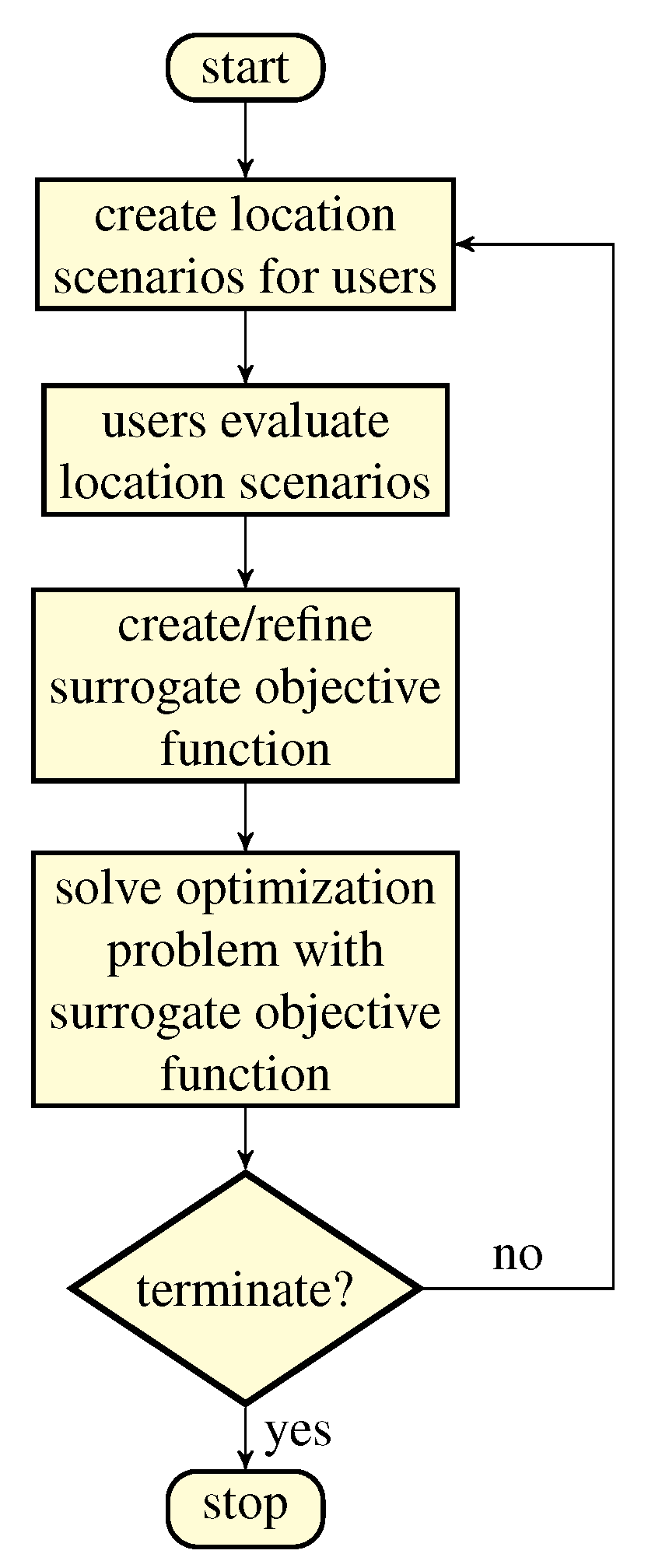
Figure 1 shows the basic methodology: In each iteration, the algorithm first generates location scenarios for a subset of users to evaluate. Based on the users’ ratings of the scenarios, a surrogate objective function is continuously updated over the iterations. The GSPDP instance with the current surrogate objective function is then solved, yielding a solution. In the next iteration, this solution is a basis for deriving further meaningful location scenarios to be presented to users again. The surrogate objective function, thus, learns to represent the users’ needs, more specifically the suitability values
, better and better, and the solutions obtained from the optimization will become more precise over time.
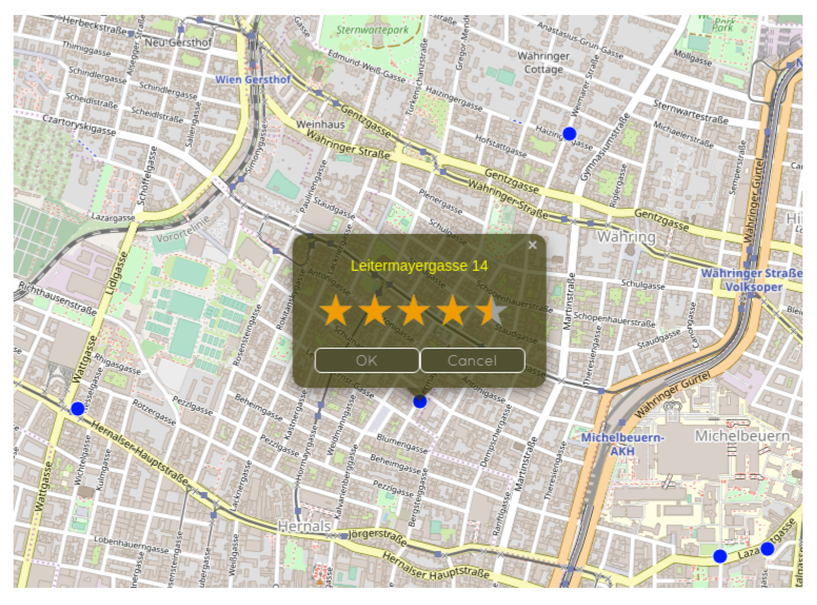
Figure 2 exemplifies how the evaluation of a location scenario may look from the perspective of a user.
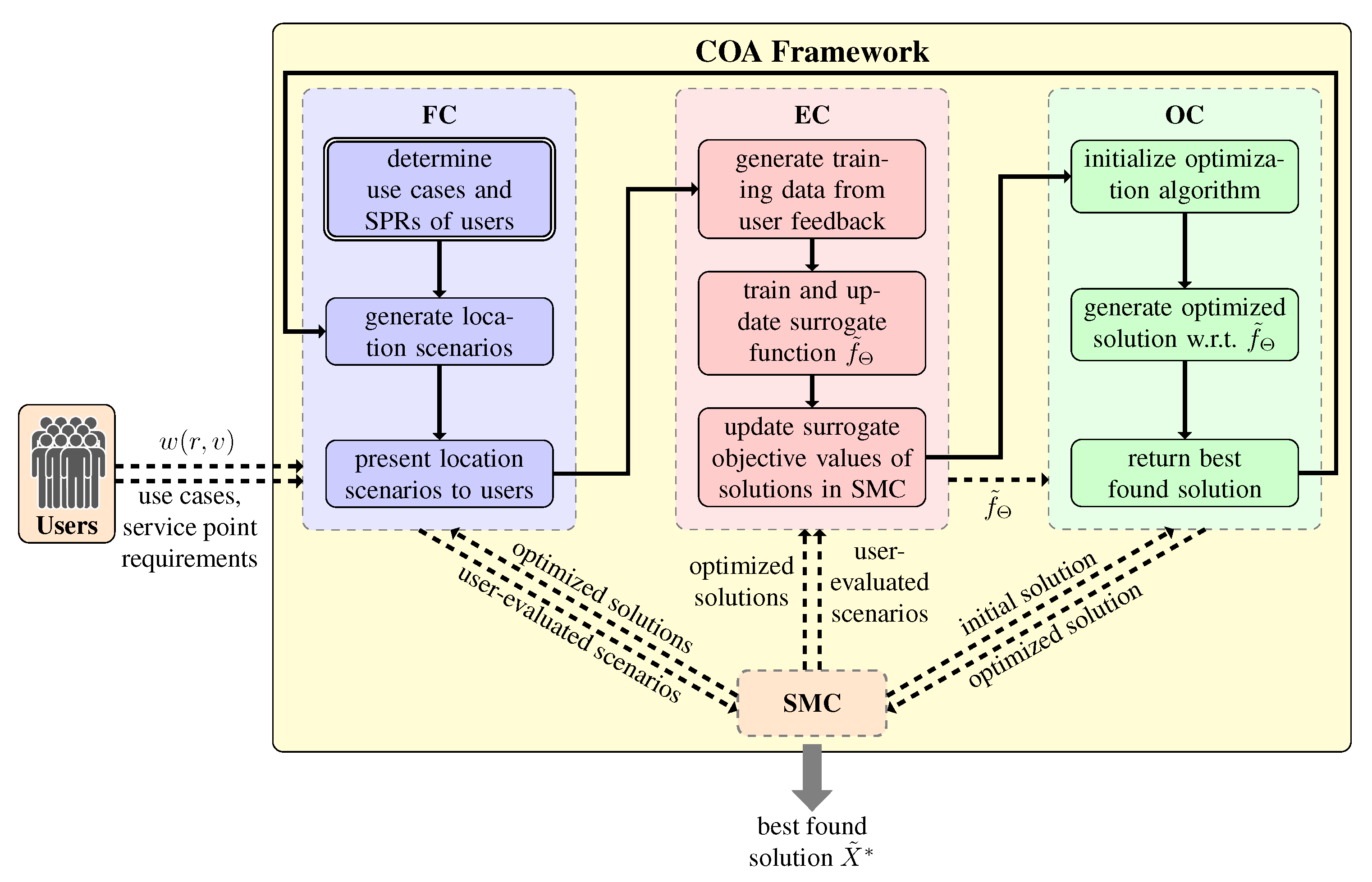
From a technical point-of-view, the COA framework consists of a Feedback Component (FC), an Evaluation Component (EC), an Optimization Component (OC), and a Solution Management Component (SMC).
First, the FC is called, starting an initialization phase by asking each user to specify the user’s use cases and associated SPRs , as well as corresponding demands , . Afterwards, the FC is responsible for collecting information from the user, i.e., users can interact with the framework at this stage of the algorithm. User information is collected by generating individual location scenarios for each user which are presented to the user in order to obtain his/her feedback. A user then has to provide suitability values for locations of solution scenarios S presented to him with respect to a use case requirement .
The feedback obtained from the users is processed in the EC. The EC maintains and continuously updates a
surrogate suitability function approximating the suitability values
of service point locations
w.r.t. SPR
without interacting with the respective user. This function is realized by a machine learning model with parameters (weights)
. Based on this surrogate function, the EC also provides the surrogate objective function
with which a candidate solution
X can be approximately evaluated. This fast approximate evaluation is particularly important for intermediate candidate solutions generated during the optimization process which are not evaluated by the users. The respective learning mechanism of the surrogate objective function is also part of the EC.
A call of the OC is supposed to determine an optimal or close-to-optimal solution to the problem with respect to the EC’s current surrogate objective function . Note that the surrogate objective function never changes during a call of the OC, only in each major iteration of the framework after having obtained new user feedback. With the exception of the first call, the optimization procedure of the OC is warm-started with the current best solution as initial solution to possibly speed up the optimization process.
Finally, the SMC efficiently stores and manages information on all candidate solutions that are relevant for more than one of the above components and, particularly, also the location scenario evaluations provided by the users so far, as well as the solutions returned by the OC.
The whole process is repeated until some termination criterion is reached, e.g., the discrepancy of user feedback and the results of the EC is small enough or a maximum number of user interactions has been reached. In the end, COA returns a solution with the highest surrogate objective value of all of the so far generated solutions.
Figure 3 and Algorithm 1 give a summary of the whole COA procedure and of the main tasks of each of the components of COA.
| Algorithm 1: Basic Framework |
Input: an instance of the GSPDP
Output: best solution found
1: Feedback Component:
2: for do
3: obtain use cases with associated demands and service point requirements , , from user u;
4: end for
5: while no termination criterion satisfied do
6: Feedback Component:
7: for each scenario generation strategy do
8: random sample of R;
9: for do
10: generate set of location scenarios according to strategy ;
11: present scenario to the corresponding user;
12: update SMC with ratings obtained from ;
13: end for
14: end for
15: Evaluation Component :
16: train surrogate model , yielding updated surrogate obj. function ;
17: re-evaluate all solutions stored in the SMC with new ;
18: Optimization Component:
19: generate optimal solution w.r.t. the EC’s ;
20: update SMC with ;
21: end while
22: return overall best found solution ;
|
In the next subsections, we describe each component’s functionality in more detail.
4.2. Solution Management Component
The SMC stores and manages so far considered solutions and evaluations by the users. The set of solutions obtained from the OC in all major iterations is stored in a set we denote by . For each solution , the SMC keeps track of its current surrogate objective value . Hence, the surrogate objective values of the solutions in are updated in each major COA iteration whenever the EC updates the surrogate suitability function. The current best solution in , i.e., the solution with the highest surrogate objective value, is denoted by .
All feedback obtained from the users via the presented location scenarios is collected and stored in the SMC in a hash map: Its set of keys, which we denote by K, is the set of pairs with for which suitability values have been obtained from the users, and the respective values are the .
Last but not least, through the FC, we are also able to obtain upper bounds on suitability values
, with
, as will be explained in
Section 4.3. These upper bounds are stored in the SMC as
.
4.3. Feedback Component
The FC is responsible for extracting as much information as possible from the users with as few interactions as necessary in order to not to fatigue them.
In the context of the COA framework, user interactions are understood as letting a user evaluate (a small number of)
location scenarios. Similar to a solution, a location scenario is a subset of locations in
V at which service stations are assumed to be opened. In contrast to a solution, the budget constraint (
1) does not need to be respected, and a location scenario may, therefore, include an arbitrary number of service points. Recall
Figure 2 for an example of how an interaction with the COA framework may look from the perspective of a user.
Let be such a location scenario provided to a user u with respect to one of the user’s SPRs . It is then assumed that the user returns as evaluation of the scenario S either a best suited location and the corresponding suitability value or the information that none of the locations of the scenario S is suitable. The latter case implies that for all . In case multiple locations are equally well suited, we assume that the user selects one of them at random. It is assumed here that the suitability of a location w.r.t. an SPR can be specified by the user on a five-valued scale from zero, i.e., completely unsuitable, to one, i.e., perfectly suitable; a more fine grained evaluation would not make much practical sense.
Clearly, this definition of user interaction is simplified and idealized, particularly as we assume here that all users always give precise answers. In a real application, the uncertainty of user feedback and the possibility of misbehaving users who intentionally give misleading answers also need to be considered among other aspects. Moreover, it would be meaningful to extend the possibilities of user feedback. For example, users could be allowed to optionally rate more than one suitable locations for an SPR in one scenario or to make suggestions which locations to additionally include in a scenario as we considered it in Reference [
13].
In each iteration of COA, users are presented with individual sets of location scenarios for their service point requirements . These scenarios are compiled according to the following strategies.
Remember that location suitability values obtained from the users are later used in the EC for training the surrogate function . Moreover, by enforcing that each user is required to select a best suited service point location in a presented location scenario for an SPR r, a suitability value indicated by the user for some location also serves as upper bound on the suitability values of all other locations in the location scenario S; thus, . By , the SMC maintains for each SPR , and each location the so far best obtained upper bound on each ; initially, .
Let be the initially unknown set of locations that are actually relevant to a user w.r.t. an SPR . A straightforward strategy to identify this set is to iteratively present the user scenarios , containing all locations for which no entry exists yet, i.e., locations for which no suitability values are known yet w.r.t. r. Following this strategy, it can be ensured to identify a new location of in every iteration of COA. Note, however, that it can only be guaranteed that is completely known once the user returns that none of the locations in the last scenario are suitable for r. Consequently, will be completely known after user interactions.
Hence, an upper bound
on the total number of required interactions with user
u for completely identifying all relevant locations for all of his/her use cases is
While this value is unknown in a real-world scenario, it allows us to establish a measure of quality on how well our strategy for presenting scenarios to users performs within our testing environments.
The same combination of two strategies for generating scenarios w.r.t. an SPR
as in Reference [
16] is used. The first strategy generates scenarios according to the approach described above, i.e,
. The second strategy generates scenarios
containing all locations from the current best solution that have not been rated yet w.r.t.
r.
Note that, for users, generally only a fraction of the service point locations in V is actually relevant to one of their SPRs. Hence, when presenting a user two scenarios for each of the user’s SPRs, every iteration, the number of user interactions would quickly exceed . Therefore, in the first COA iteration, a scenario is generated for each , but, in successive iterations, scenarios are only generated for subsets of R. More specifically, from the second iteration onward, and percent of the SPRs are randomly selected for generating scenarios according to and , respectively, with and being strategy parameters.
4.4. Evaluation Component
The EC processes the user feedback obtained from the FC and provides the means for evaluating candidate solutions without relying on users in particular within the OC. The exact objective function
f from (
2), which is based on the mostly unknown suitability values
with
, is approximated by the surrogate objective function
, cf. (
11), making use of the following
surrogate suitability functionGenerally speaking,
is here a learnable function with weight parameters
approximating
for all unknown pairs
. The above definition, thus, ensures that
always returns known values
and otherwise respects lower bounds zero and upper bounds
, giving function
g more freedom. Upper bounds
are initially set to one. In
Section 4.3, discussion is given on how tighter upper bounds are derived.
Suitability values are approximated by exploiting similarities of SPRs among users. In general, we cannot expect that there exist users having the same needs in all respects, i.e., the users have the very same use cases with the same demands. However, given a sufficiently large user base, it is realistic that there are users having similar SPRs and associated preferences concerning suitable locations.
A popular collaborative filtering technique for exploiting similarities among user preferences is
matrix factorization [
39], which we also apply here. Given an incomplete matrix containing ratings
for a set of users
U over a set of products
P, the idea behind matrix factorization is to decompose this matrix into two smaller matrices, a user/feature matrix
and a product/feature matrix
, such that the product of these two matrices approximates the original matrix. An unknown rating, i.e., a rating not contained in the original matrix
, can then be estimated as the dot product of the corresponding feature vectors in matrix
and matrix
, respectively.
Moreover, we also want to exploit the fact that only a small fraction of the locations in
V is typically relevant for the SPR of a user and that unknown ratings are not missing at random. In our problem users are always asked to rate the most suitable location of a scenario. Therefore, known ratings tend to be biased towards more positive values, while unrated locations are likely to have a low suitability for a user w.r.t. an SPR. A matrix factorization approach that takes such considerations into account has been suggested by Reference [
17]. Traditionally, the rating matrix
is factorized by solving the optimization problem
where
E is a loss function for measuring the error between the actual and the predicted ratings, and
is a regularization term. In Reference [
17], this minimization problem is expanded by adding a bias term for unknown ratings towards a certain value
, i.e.,
Parameter controls the impact of this new term in the optimization. The authors show for selected loss functions how this new optimization problem can be solved in the same time complexity as the traditional optimization problem.
In order to apply matrix factorization for approximating suitability values in our case, we start from the sparsely filled matrix containing all so far known suitability values. By factorizing W along the r dimension and the v dimension on the basis of a feature set , we obtain an SPR/feature matrix with and a location/feature matrix with . Feature vectors describe the SPR r in terms of abstract features, while feature vector reflect the characteristics of locations v. In general, it is expected that SPRs with similar needs will have similar feature vectors in , and locations with similar suitability characteristics will have similar feature vectors in . The number of features is hereby a parameter that is chosen, e.g., in dependence of an estimation of the overall number of different service point requirements, and we assume it is considerably smaller than the overall number of SPRs, as well as the number of locations n. As unknown suitability values are more likely zero than being greater than zero, we set the bias target .
Having obtained matrices
and
, an unknown value of
W is approximated by the dot product of the respective feature vectors rounded to the nearest of the five discrete suitability values we defined, i.e.,
The trainable parameters of are, therefore, .
Our loss function for the matrix factorization is
and randomized block coordinate descent [
47] is used to minimize it.
4.5. Optimization Component
Recall that the OC is performed in each major iteration of the framework and makes use of the current surrogate objective function provided by the EC, whose weights do not change during each individual call of the OC. The OC is, thus, supposed to return an optimal or close-to-optimal solution to our problem w.r.t. the current surrogate objective function.
In our implementation of the OC, we apply a general purpose MILP solver to the MILP formulation already presented in
Section 3, Equations (
3)–(10); however, suitability values are approximated by the surrogate suitability function
. Note that, for improved scalability, a metaheuristic approach might also be used as optimization core as it is not necessary to find an optimal solution in each iteration. However, due to the complexity of the objective function of the GSPDP, such a metaheuristic requires significant effort to be able to scale well to larger instances. As the development of such a heuristic would go beyond the scope of this paper, we, therefore, leave this task for future work.
5. Test Cases
The following describes how test instances for evaluating COA have been generated. Instead of testing with real users, user interaction is simulated in an idealized manner in certain test cases in order to analyze the strengths and weaknesses of the framework with a focus on the algorithmic aspects. The considered test instances are of three groups. The first two groups are purely artificial test instances inspired by the location planning of stations for electric vehicle charging, denoted by EVC, and, for (station-based) car sharing systems, denoted by CSS, respectively. While, in group EVC, each use case has one SPR, there are always two SPRs per use case in CSS. The third group of test instances is designed similarly to group CSS, also addressing the car sharing scenario, but the instances are generated from real-world taxi trip data of Manhattan; this group is, therefore, called MAN. Note that COA intentionally does not make use of geographic information in any of its components. Therefore, modeling preferences of users for our instances in dependence of the proximity to service point locations does not provide COA any advantage for finding an optimized solution.
5.1. Artificial Test Instance Groups EVC and CSS
Test instances from the groups EVC and CSS are generated with the same approach. The n possible locations for service stations are randomly distributed in the Euclidean plane with coordinates , chosen uniformly from the grid , with . The fixed costs , as well as the variable costs for setting up a service station at each location , are uniformly chosen at random from . The budget is assumed to be so that roughly 10% of the stations with average costs can be expected to be opened.
The number of use cases for each user is chosen randomly according to a shifted Poisson distribution with offset one, expected value three, and a maximum value of five, i.e., the number of use cases never exceeds five. Each of these use cases is associated with an individual demand randomly chosen from {5,…,50} and, depending on the benchmark group, with one (EVC) or two (CSS) SPRs.
Each SPR
of a use case
c also is associated with a particular geographic location
. In order to model similarities in the users’ SPRs, these locations are selected in the following correlated way. First, ten
attraction points A with uniform random coordinates are selected from
. Then, each use case location is derived by randomly choosing one of these attraction points
and adding a small individual offset to the coordinates, i.e.,
where
denotes a random value sampled from a normal distribution with the respectively given mean value and standard deviation
. If obtained coordinates are not in
, a new attraction point is chosen, and the deviation is re-sampled.
A service point location
receives a rating w.r.t. an SPR
r, according to a sigmoidal decay function applied to the Euclidean distance, and is also perturbed by a Gaussian noise with a standard deviation of
:
The parameters of the sigmoid function are chosen so that
decreases as the distance between
v and
increases and becomes approximately zero at a distance larger than twelve. Additionally, as motivated in
Section 3, we discretize the rating
by rounding to the closest value in
, obtaining
. Hence,
.
Six sets of 30 benchmark instances were generated for EVC, as well as CSS. As detailed in
Table 1, these sets consider
potential service point locations in combination with different numbers of users and two different settings for the standard deviations of the Gaussian perturbations
and
. Note that parameters
and
control how similar suitability values for locations of SPRs generated from the same attraction point are. The larger
and
, the more different are the preferences of the users. Hence, we have chosen two different settings for
and
to show how COA behaves under conditions in which preferences of users towards locations for service points have a higher and lower similarity, respectively. Values for
and
have been determined experimentally in preliminary tests. In the following, we will denote instance sets primarily by the pair
.
5.2. Manhattan Test Instances
Next to the above described purely artificial benchmark instances, we also derive benchmark instances from real-world yellow taxi trip data of Manhattan. As in CSS, MAN instances have two SPRs per use case. The underlying street network
G of the instances corresponds to the street network graph of Manhattan provided by the Julia package LightOSM (
https://github.com/DeloitteDigitalAPAC/LightOSM.jl, accessed on 10 June 2021). Taxi trips have been extracted from the 2016 Yellow Taxi Trip Data (
https://data.cityofnewyork.us/Transportation/2016-Yellow-Taxi-Trip-Data/k67s-dv2t, accessed on 10 June 2021). The taxi data set was first preprocessed by removing all trips with invalid data and trips made on a weekend. Furthermore, we have also removed all trips which do not start, as well as end, in Manhattan. For taxi trips within the months of January to July, geographic pickup and drop-off coordinates of customers are recorded in the data set. Each of these coordinates has been extracted and mapped to the geographically closest vertex in
G, resulting in a list of pairs of vertices
. Next, as the similarity of users in our instances depends on their geographic proximity, we have reduced
Q by considering only the ten taxi zones with the highest total number of pickups and drop-offs of customers, resulting in a total of approximately two million taxi trips. Geographic information of the taxi zones of Manhattan has been obtained from
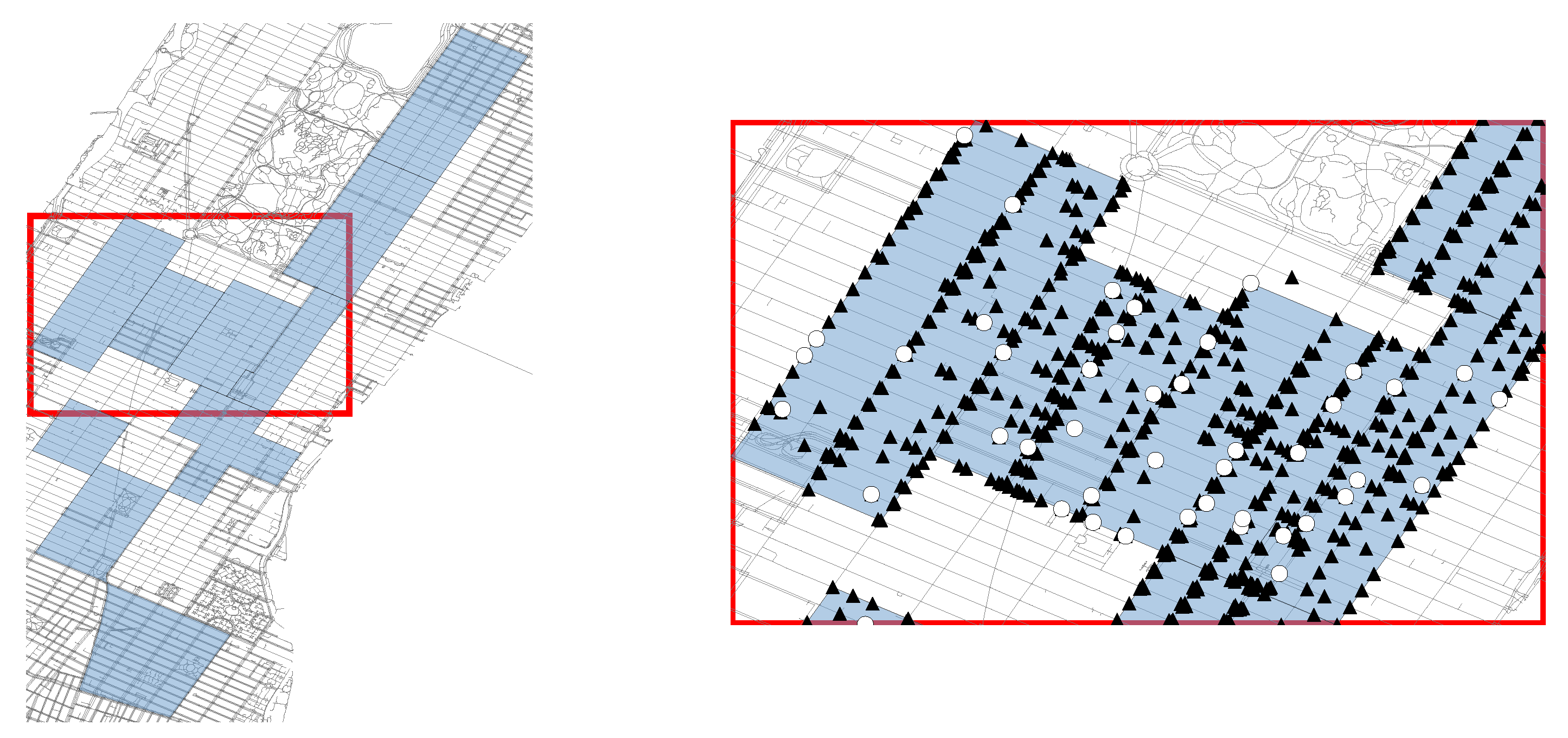
https://data.cityofnewyork.us/Transportation/NYC-Taxi-Zones/d3c5-ddgc (accessed on 10 June 2021). The left side of
Figure 4 provides a visualization of the selected taxi zones.
The set of potential service point locations V has been chosen randomly from vertices of G that are located in the considered taxi zones. The fixed costs , as well as the variable costs , for setting up a service station at each location , are uniformly chosen at random from .
The number of use cases for each user
is again chosen randomly according to a shifted Poisson distribution with offset one, expected value three, and a maximum value of five. Each of these use cases
is associated with an individual demand
randomly chosen from
and the two SPRs representing the origin and destination of a trip chosen from
Q uniformly at random. A rating for an SPR
r is calculated for each
via the sigmoidal decay function
where
refers to the length of the shortest path between location
v and the SPR
r in the street network graph
G. The parameters of this function have been chosen in such a way that service point locations within a distance of approximately 600 meters to
r are relevant for the SPR. Finally, the discretized suitability value
is again obtained by
. The right side of
Figure 4 shows the distribution of SPR locations, as well as potential service point locations, as an example instance.
The MAN benchmark group consists of 30 instances in total with each instance having 100 potential service point locations and 2000 users. Additionally, each instance will be evaluated with different budget levels such that about b percent of the stations considering average costs can be opened, i.e, the actual budget for each instance is calculated as .
6. Results
The COA framework including the FC were implemented in Python 3.8. For the matrix factorization of the EC, we adapted the C++ implementation of Reference [
17] provided on Github (
https://github.com/rdevooght/MF-with-prior-and-updates, accessed on 10 June 2021). The parameterization of the COA components have been determined through preliminary tests on an independent set of instances. For all test runs, the weighting for unknown suitability values
of the matrix factorization has been set to one. Moreover, the number of features considered in the matrix factorization is set to ten for all test runs. The parameters
and
for controlling the number of scenarios generated according to each strategy in the FC have been set to
and
, respectively. Finally, Gurobi 9.1 (
https://www.gurobi.com/, accessed on 10 June 2021) was used to solve the MILP models in the OC. In each COA iteration, a time limit of ten minutes has been set for solving the MILP. If the MILP was not solved to optimality within this time limit, the best found solution was used. All test runs have been executed on an Intel Xeon E5-2640 v4 2.40 GHz machine in single-threaded mode with a global time limit of four hours per run. Note, however, that all runs terminated within this time limit once all relevant locations had been discovered. Since, in contrast to COA, we have full knowledge of our test instances, we are also able to calculate optimal reference solutions for each instance. Hence, by
, we denote the objective value of a respective optimal solution
.
To characterize the amount of user interaction performed by COA, we consider the total number of scenarios evaluated by a user
in relation to the upper bound of required interactions
, cf.
Section 4.3. Let
be the number of user interactions of user
performed within COA to generate some solution. Then,
refers to the relative average number of performed user interactions relative to
over all users. Note that since scenarios are presented only to a fraction of users in every iteration, the average number of user interactions at each iteration of COA varies even for instances within the same benchmark group. Hence, in order to reasonably study results for each of our benchmark groups, we aggregate respective results to our instances at various
interaction levels by selecting for each instance the COA iteration at which
I is largest but does not exceed
. Note that, for some instances, smaller levels of
are already exceeded in the first iteration of COA. Hence, in the following, we only consider interaction levels for an instance group for which results to all corresponding instances exist.
Note further that the user interaction levels can also be interpreted as the average information known about a user. This interpretation allows us to draw a direct comparison to traditional approaches for distributing service points in which information about the demands of the users is determined in advance. Each result at a certain interaction level can also be interpreted as the result of such a traditional approach with a certain level of knowledge about the users. However, to the best of our knowledge, there exists no data about suitability values in other work. Additionally, for a fair comparison between COA and other approaches from literature, one would have to also take into account the costs required for obtaining said information about the users. Therefore, comparing COA to other approaches from literature seems to be not possible without an extensive study on suitability values of users or a complex simulation of users based on various assumptions that can heavily influence the outcome of such a comparison.
First, we want to show how the quality of incumbent solutions develops as the number of user interactions increases during a COA run. For this purpose, we calculate the optimality gap for a solution
x obtained from COA as
.
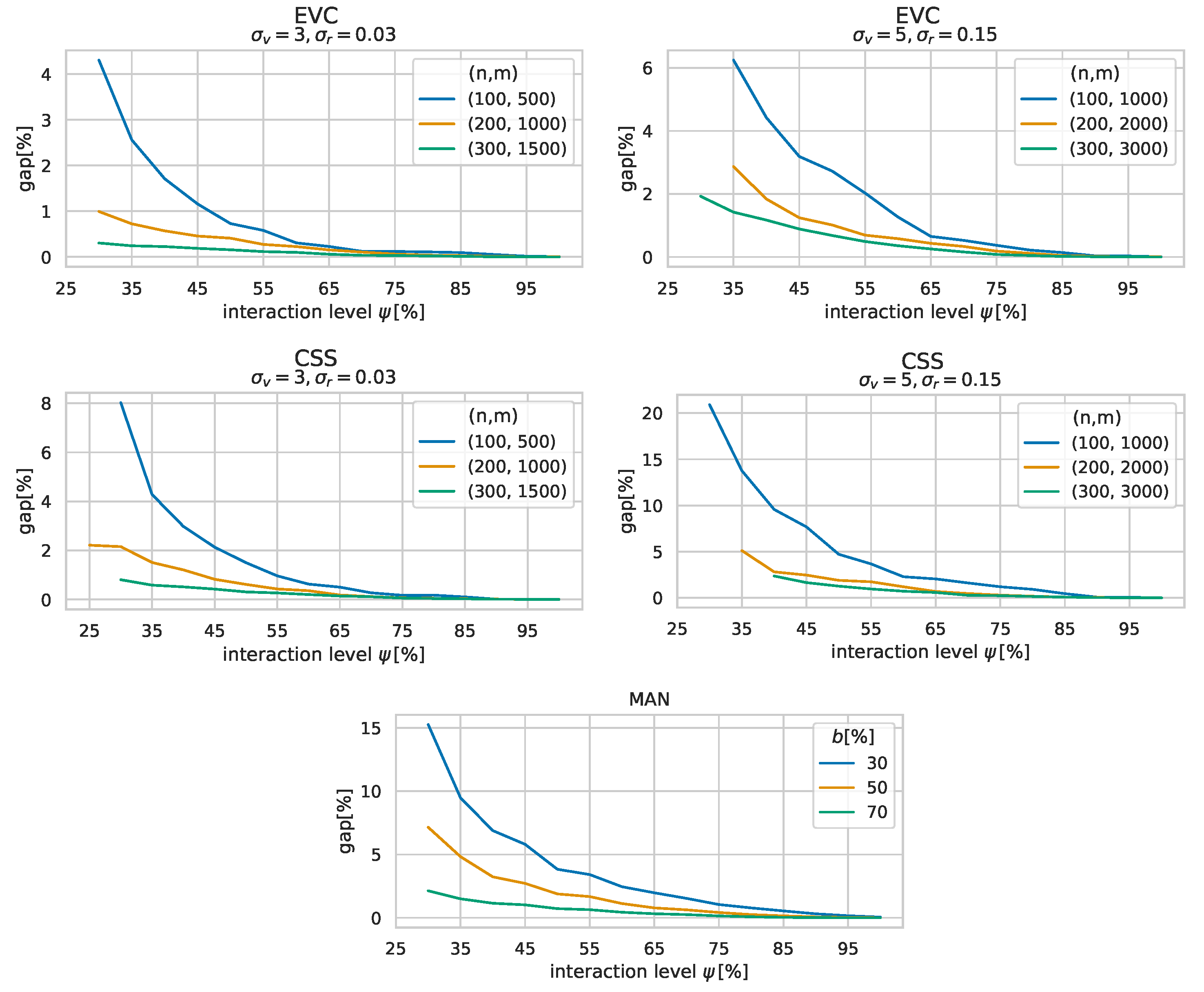
Figure 5 shows the average optimality gaps of solutions to each of our benchmark sets against the interaction levels
. The results are grouped by
and
to additionally compare instances groups with similar user behavior.
Recall that the number of attraction points is the same for all EVC and CSS instances. Therefore, for instances with a higher number of users, it is generally easier to find better solutions as there are more users that prefer the same locations. The plots show that, in all cases, solutions generally improve quickly with an increasing interaction level, and close to optimal solutions can be obtained well before identifying all the users’ relevant locations. Specifically, at a user interaction level of 50%, the solutions generated by COA feature optimality gaps of 1.45% on average. An exception of this observation are the MAN instances with . For these, generated solutions do not reach an optimality gap below before , on average. Moreover, the figure also shows that the solutions to MAN instances generally converge notably slower than the solutions to EVC and CSS instances. This behavior is likely caused by the weaker correlation of user preferences in the MAN instances and the way that the FC generates scenarios presented to the users, specifically the aspect that locations important to the individual users are tried to be identified first. Locations important to individual users might not necessarily be the best locations to add to a solution, especially if there is a lower number of users with similar preferences. Consequently, the strategies based on which scenarios are generated may still have some room for improvement for such cases. Instead of primarily identifying locations important to users, targeting locations in relation to the current best solution with a higher emphasis might be a more expedient approach here.
Note that an increased number of user interactions does not only imply a larger trainings set for the surrogate function but also results in better upper bounds
for locations
w.r.t. to an SPR
. Therefore, to gain a better understanding of how much the surrogate function actually contributes to finding an optimized solution, we study what happens when the learning surrogate suitability function
is replaced by the naive function with no learning capabilities
In the following, we refer to our original COA implementation with the surrogate function
as COA
and denote the implementation with the naive function
as COA
. A comparison between COA
and COA
is shown in
Table 2. Each table cell shows the average optimality gaps of solutions to the respective instance group at the specified interaction levels
. The better results among COA
and COA
are printed bold. Additionally, as the standard deviations w.r.t. the optimality gaps are quite large, shown in
Figure 6, we have also applied a one-sided Wilcoxon signed-rank test to determine for each group, whether the difference in optimality gaps is significant or not. Instance groups for which the Wilcoxon test has assessed at a 95% confidence interval that either COA
or COA
has produced better optimality gaps are marked with an asterisk.
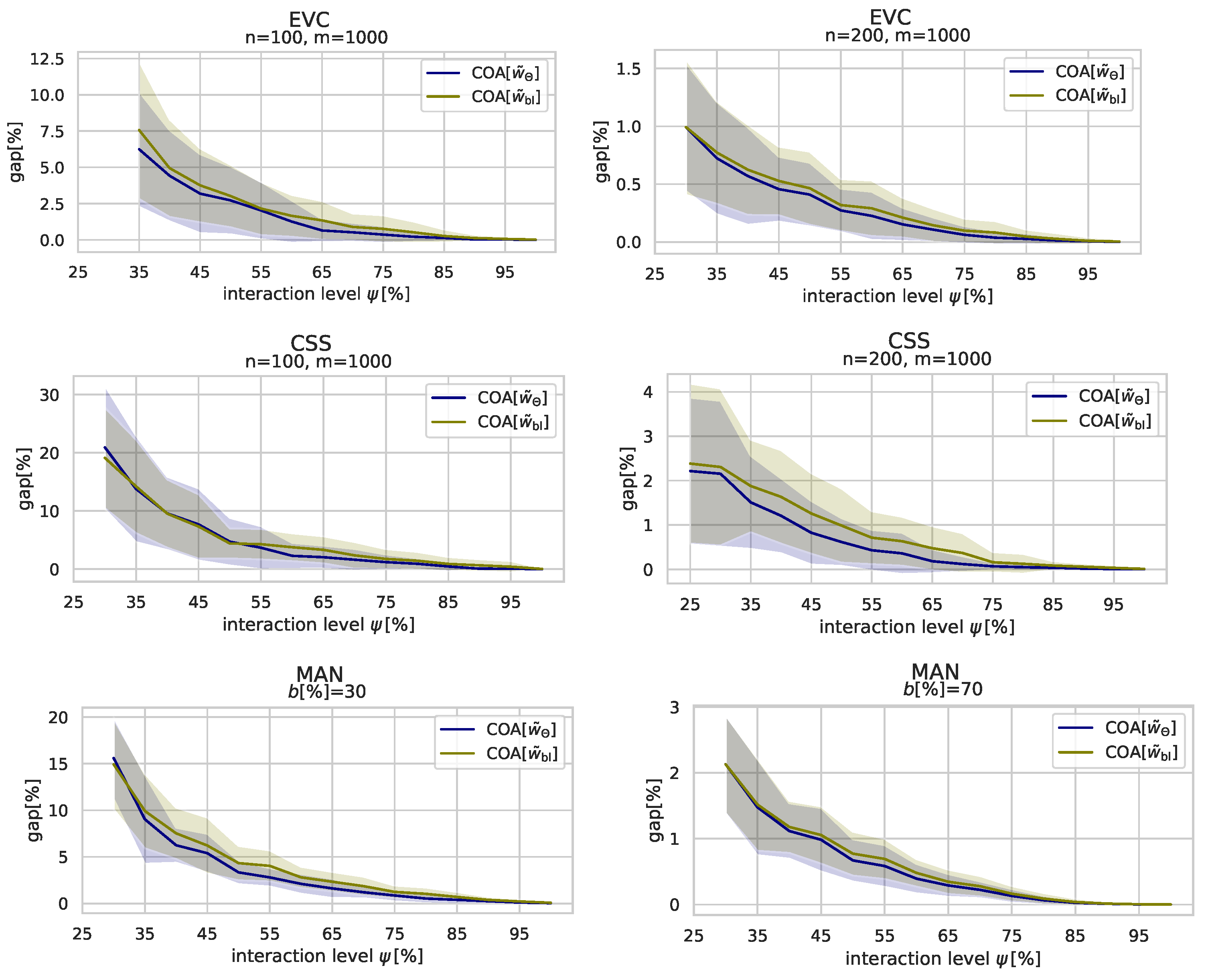
The table shows that, especially for the CSS and MAN instances, COA generates significantly better results at almost all interaction levels than COA. While, for the EVC instances, the average optimality gaps w.r.t COA are lower than the average optimality gaps w.r.t. COA, there are instance groups for which no significant difference between the optimality gaps can be determined. However, there is no instance group for which COA produced significantly better results than COA with over all user interaction thresholds. It can be observed that, at very low levels of user interaction, COA and COA seem to be equally strong. However, as the amount of collected of user feedback increases, COA quite quickly outperforms COA.
Figure 6 gives a visual comparison between COA
and COA
for selected instance groups and not only shows average optimality gaps but also respective standard deviations around the mean values as shaded areas. The figure confirms that the average gaps produced by COA
are generally lower than those of COA
but also shows that the standard deviations are quite large in general for both approaches. However, as COA progresses and the quality of the solutions improves, the standard deviations decrease, as well.
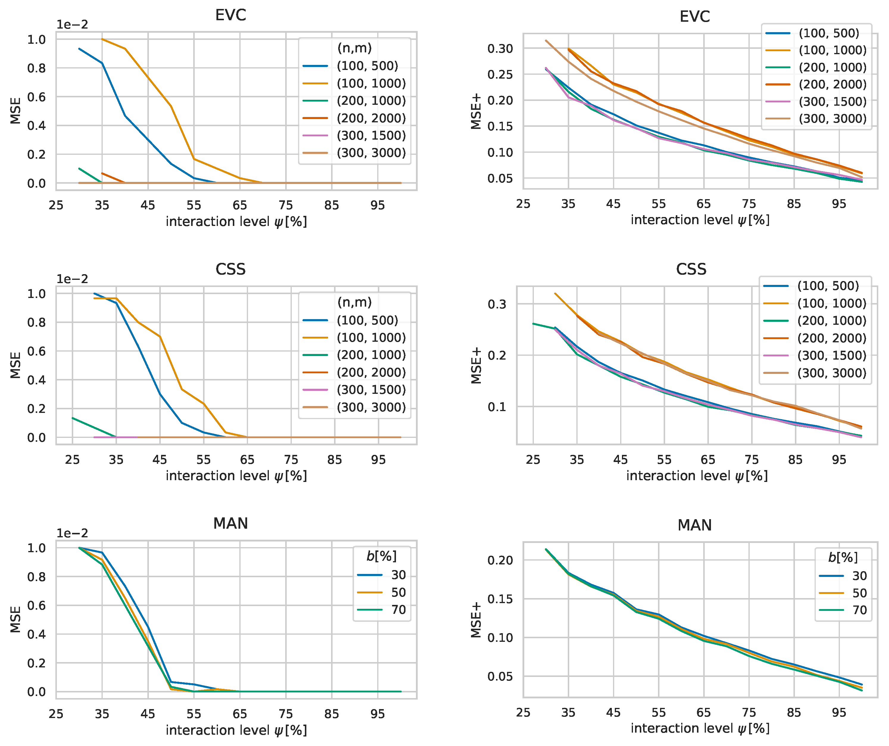
To further investigate the learning capabilities of the surrogate function, we now look at the mean squared error (MSE) of
with respect to the known exact values
w. The left plots in
Figure 7 show the development of this MSE calculated over all suitability values that are not known yet by COA for all instance groups. It can be seen that the MSE is generally small and approaches zero rather quickly. The reason for such small values can be found in the matrix factorization model used in the EC, which adds a bias for unknown suitability values towards zero as users typically only have a small number of locations with positive suitability values for each of their SPRs. Consequently, the MSE is distorted by the large number suitability values that are zero.
Therefore, the plots on the right side of
Figure 7 show average mean squared errors calculated only over all
positive suitability values that are not known yet; we denote this error by MSE+. This measure gives a clearer picture on how the surrogate function continuously improves in all cases with an increasing amount of gained knowledge. At the start of the algorithm the MSEs of the benchmark groups are between
and
on average and go towards zero almost linearly with the interaction level. Note that neither the size of an instance nor the given budget seem to have a significant impact on the size of the errors. Additionally, the figure also highlights how the instance parameters
and
impact the similarity of user preferences as the MSEs for instances with
and
are generally larger than the MSEs for instances with
and
.
Finally, in
Table 3, we also compare COA
to the COA implementation using the surrogate function
introduced in Reference [
16], henceforth referred to as COA
. While
is also based on a matrix factorization model, this model does not take into account that user data is not missing at random.
Each table cell shows the average optimality gaps of solutions to the respective instance set at the specified interaction level . The better results among COA and COA are printed bold. A one-sided Wilcoxon signed-rank test was used to determine for each instance set whether the difference in optimality gaps is significant or not. Entries for which the Wilcoxon test has assessed at a 95% confidence level that either COA or COA has produced better optimality gaps are marked with an asterisk. It can be observed that, for lower levels of user interaction, solutions generated by COA exhibit extremely high optimality gaps. However, the higher the number of user interactions, the more COA can catch up with COA. However, most of the time, COA still dominates COA. Summarizing, it can be concluded that the new matrix factorization model is a significant improvement over our previous model , resulting in COA generating better solutions with fewer user interactions than COA most of the time.
7. Conclusions and Future Work
In this paper, the previously introduced Cooperative Optimization Algorithm was generalized to be applicable to more application scenarios and to larger instances with hundreds of potential service station locations and thousands of users. New application scenarios include, in particular, those in which the fulfillment of a single demand depends on more than one suitably located service points as it is the case in station-based bike and care sharing. Results on artificial and real world inspired instances show how the solution quality improves as the amount of user feedback increases and that a near optimal solution is reached for most instances with a reasonably low amount of user interactions. To characterize the amount of user interaction performed by COA, we have established an upper bound on the maximum number of non-redundant user interactions and introduced the notion of user interaction levels. Solutions generated by COA feature optimality gaps of 1.45% on average at an interaction level of 50%. Furthermore, we could clearly observe that the matrix factorization-based surrogate model is able to learn preferences of individual users from users with similar interests. More specifically, we made use of an advanced matrix factorization model which takes into account that user data is not missing at random. In fact, users are always asked to rate the most suitable location of a scenario, if one exists. The experimental comparison indeed confirmed the benefits of this new model over the original one, especially when the interaction level is still low. Using the new matrix factorization model, COA is able to generate better solutions with fewer known user preferences than before. In addition, note that, while we achieve our best results with the matrix factorization-based surrogate model, the results also show that COA already works reasonable even without learning user preferences.
However, there is still potential left for future improvements. In our COA implementation, the strategies by which scenarios for users are generated favor the selection of unrated locations that may be important for individual users but not necessarily for a global optimal solution. In order to quickly find a good solution by the optimization, it is important for our surrogate function to have higher accuracy for locations that have the potential to actually appear in a globally optimal solution. Otherwise, finding a near optimal solution requires a larger amount of user interactions as we have observed in our results on the Manhattan instances. In order to improve the scenario generation strategies, it seems natural to enrich the feedback component (FC) with knowledge not only from the evaluation component (EC) but also from the optimization component (OC). As the OC finds optimized solutions via a MILP, utilizing dual solution information, such as reduced costs or performing a sensitivity analysis, might be a promising direction.
It would also be interesting to further improve the scalability of COA. While a time limit of ten minutes per MILP was still sufficient for solving our benchmark instances, the OC is the main bottleneck of COA w.r.t. computation times. On the one hand, one can resort to heuristic optimization approaches in the OC. On the other hand, hierarchical clustering and multilevel refinement strategies as applied in the context of planning a bike sharing system in Reference [
2] appear promising.
COA was applied for generating solutions to instances of the General Service Point Distribution Problem (GSPDP). While we have proven the GSPDP to be NP-hard, this problem is rather abstract and, from a practical perspective, still too simplistic. For a specific practical application, the problem formulation needs to be tailored appropriately. Diverse aspects, such as different configuration options of stations, capacities, or time-dependent aspects, may be needed to be considered. To a certain degree, the general framework of COA can stay the same or may need only smaller adaptions, such as in the scenario generation of the FC.
Finally, we want to emphasize that the focus of this contribution was on the algorithmic and computational aspects of COA and its components. Clearly, further challenges concern a suitable user interface and a corresponding distributed implementation of at least the FC, in which also psychological aspects of users need to be considered. Moreover, the performed experiments are based on the assumption of perfect user feedback, which does not hold in practice. The impacts of not entirely reliable evaluation results need to be studied, and robust variants of certain components of COA need to be devised.


