A Greedy Heuristic for Maximizing the Lifetime of Wireless Sensor Networks Based on Disjoint Weighted Dominating Sets

Abstract

Dominating sets are among the most well-studied concepts in graph theory, with many real-world applications especially in the area of wireless sensor networks. One way to increase network lifetime in wireless sensor networks consists of assigning sensors to disjoint dominating node sets, which are then sequentially used by a sleep–wake cycling mechanism. This paper presents a greedy heuristic for solving a weighted version of the maximum disjoint dominating sets problem for energy conservation purposes in wireless sensor networks. Moreover, an integer linear programming model is presented. Experimental results based on a large set of 640 problem instances show, first, that the integer linear programming model is only useful for small problem instances. Moreover, they show that our algorithm outperforms recent local search algorithms from the literature with respect to both solution quality and computation time.

1. Introduction

Wireless sensor networks (WSNs) have received increasing attention in the last decade due to their potential applications in various fields such as environmental monitoring, medical and health applications, security surveillance and emergency operations [1]. They are generally composed of a rather large number of small devices, called sensors, with a limited low-power supply that depletes rather quickly. The lifetime of a sensor device (in hours) is generally calculated by dividing the battery capacity (in Watt hours) by the average power drain (in Watts). However, as the energy consumption also depends on other factors—such as, for example, the operating temperature—the estimation of the lifetime of a sensor node is not trivial [2]. One of the most challenging issues in WSNs is extending the lifetime of the network while providing sufficient sensing coverage and communication reliability. The lifetime of a network is defined as the time (duration) in which the network is fully functional with respect to the tasks that have to be fulfilled, that is, the time duration in which the overall sensing coverage is maintained. Therefore, WSN lifetime significantly depends on the energy consumption of sensors in the context of limited energy availability. Examples of real-world applications for maximizing sensor network lifetime can be found in [3] (human activity monitoring), [4] (smart agriculture monitoring), [5] (road traffic monitoring), and [6] (structural health monitoring).

According to [7], power saving strategies can usually be classified under one of the following mechanisms:

• Sleep–wake cycling (also called duty cycling): Sensors switch between active and sleep mode.
• Power control by adjusting the transmission range of wireless nodes.
• Energy efficient routing, and data gathering.
• Reducing the amount of transmitted data and avoiding useless activity.

This study focuses on the first possibility, in the following way. The problem of extending (prolonging) WSN lifetime is addressed by organizing the sensors into a number of disjoint subsets that are activated successively. We require that each of these subsets is a dominating set of the communication graph defined by a sensor network. Note that, given the locations of the sensors, the communication graph is obtained by joining two sensors with an edge in case they can communicate with each other via their wireless antennas. The requirement of a subset of sensors being a dominating set is introduced such that each subset of nodes is able to cover the whole coverage area.

The maximization of network lifetime has been studied in the literature from different perspectives. Most of them addressed the problem either via the set K-cover problem (also known as the target coverage problem) or as the domatic partition problem (also known as the maximum disjoint dominating sets problem). Slijepcevic and Potkonjak [8] were the first ones to model the problem as a set K-cover problem and proved its NP-hardness using a polynomial time transformation from the minimum cover problem. The set K-cover problem is defined over a bipartite graph of two node sets (sensors and targets) with the aim to partition the sensors into a maximum number of disjoint sets (covers) over all targets. These sensor covers are then activated one after the other to effectively extend the WSN lifetime. The sensors of an active cover are able to monitor the entire set of targets. Due to the hardness of the problem, a variety of approximate algorithms have been devised, also for different variants of the problem. Examples include a greedy heuristic [8], memetic algorithms [9,10,11], cuckoo search [12] and a genetic algorithm [13].

As mentioned before, the maximization of the lifetime of WSNs is often approached through the domatic partition problem in which the goal is to find a partition of the nodes of a given network—represented as a simple, undirected graph—into a maximum number of disjoint dominating sets. Throughout this paper, we refer to the domatic partition problem as maximum disjoint dominating sets (MDDS) problem. The MDDS problem, which belongs to the large and important family of dominating set problems [14,15,16], is known to be NP-hard for general graphs [17]. Cardei et al. [18] proved the NP-completeness of one of its variants known as the 3-disjoint dominating sets problem that asks for deciding whether or not a given graph contains three disjoint dominating sets. The same authors showed that, unless P = NP, the MDDS problem has no polynomial-time approximation with a performance guarantee of less than 1.5. They also introduced a heuristic approach based on graph coloring. In the same year, Feige et al. [19] proved that every graph of order n with maximum degree $\Delta$ and minimum degree $\delta$ includes a domatic partition (a collection of disjoint dominating sets) of size $(1-o(1\left)\right)(\delta +1)/ln\Delta$. Here, the term $o\left(1\right)$ tends to zero as n increases. Moreover, they showed that there is no approximation algorithm for the MDDS problem with an approximation ratio of $(1+o(1\left)\right)lnn$ unless $NP\subseteq DTIME\left(n^{O(loglogn)}\right)$. The same authors also provided a centralized algorithm to find a domatic partition of size $\mathsf{\Omega }(\delta /ln\Delta )$. Based on this later work, Moscibroda and Wattenhöfer [20] defined the MDDS problem as the maximum cluster-lifetime problem and introduced a randomized, distributed algorithm that has—with high probability—a performance ratio of $O(log(n\left)\right)$. Nguyen and Huynh [21] demonstrated that the 3-disjoint dominating sets problem remains NP-complete even for planar unit disk graphs and studied the performance comparison of four greedy heuristics for the MDDS problem. In [22], a greedy heuristic of time complexity $O\left(n^3\right)$ is described. More recently, Pino et al. [23] focused on a weighted variant of the MDDS problem which is henceforth labelled the maximum weighted disjoint Dominating Sets (MWDDS) problem. In this problem, each node of the input graph—corresponding to a deployed sensor device—carries a weight that corresponds to its remaining lifetime. The lifetime of a dominating set is then defined as the minimum of the lifetimes of the nodes that form part of the set. The optimization goal of the MWDDS is to find a domatic partition such that the sum of the lifetimes of the corresponding dominating sets is maximized. Pino et al. devised three local search algorithms for the MWDDS problem. Each local search algorithm is seeded with an initial feasible solution generated by a modified greedy heuristic from [22] and iteratively swaps nodes between different dominating sets in the solution, in the hope to increase the total lifetime of the network. These local search approaches differ in the way they realize the swaps.

The main contributions of this paper can be summarized as follows:

• We introduce an integer linear programming (ILP) model for the MWDDS problem.
• We propose an efficient greedy heuristic for the MWDDS problem.
• We conduct comprehensive experiments on a set of 640 problem instances in order to investigate the performance and the advantages of our greedy heuristic in comparison to the application of CPLEX and to recent state-of-the-art methods.

The rest of this paper is organized as follows. In Section 2 we provide a technical description of the MWDDS problem and recall some required notations and basic definitions. Next, an ILP model for the MWDDS problem is presented in Section 3. In Section 4, we introduce a new greedy algorithm. Finally, in Section 5 we present and discuss the experimental results, while Section 6 summarizes the work and offers directions for future work.

2. The Maximum Weighted Disjoint Dominating Sets Problem

Let $G=(V,E,\mathit{lifetime})$ be a simple, undirected, node-weighted graph, where V (with $\left|V\right|=n$) is the set of nodes, $E\subseteq V\times V$ (with $\left|E\right|=m$) is the set of edges, and $\mathit{lifetime}:V\to {\mathbb{R}}^{+}$ is a weight function that assigns a positive weight value $\mathit{lifetime}\left(v\right)>0$ to each node $v\in V$. Note that such a graph may represent the communication graph of a WSN, and the node weight may represent the lifetime of the node. However, before technically introducing the MWDDS problem, let us briefly recall some basic definitions and notations used throughout this paper. For more details on graph theoretic aspects, the readers may refer to [24]. We say that two nodes $v\ne u\in V$ are neighbors (adjacent to each other) if and only if there exists an edge between them, that is, $(v,u)\in E$. Given a node $v\in V$, $N\left(v\right):=\{u\in V\mid (v,u)\in E\}$ denotes the set of neighbors of v, known as the open neighborhood of v in G. Furthermore, the closed neighborhood of a node $v\in V$, denoted by $N\left[v\right]$, contains the nodes adjacent to v plus node v itself, that is, $N\left[v\right]:=N\left(v\right)\cup \left\{v\right\}$. The degree $deg\left(v\right)$ of v is the number of neighbors of v, that is, $deg\left(v\right):=\left|N\right(v\left)\right|$. More generally, given a subset of nodes $D\subseteq V$, the open neighborhood of D denoted by $N\left(D\right)$ is defined as ${\bigcup }_{v\in D}N\left(v\right)$ and its closed neighborhood, denoted by $N\left[D\right]$, is defined as $N\left[D\right]:=N\left(D\right)\cup D$.

Definition 1

(Dominating set). A subset $D\subseteq V$ of the nodes of a simple, undirected graph $G=(V,E)$ is called a dominating set of G if and only if each node $v\in V\setminus D$ has at least one neighbor in D. Each node in a dominating set D is called a dominator, otherwise it is called a dominatee. A dominator dominates (covers) itself and all its neighbors.

Note, for example, that—given a simple, undirected graph $G=(V,E)$—the complete set of nodes (V) is a dominating set.

Definition 2

(Domatic partition). A set $\mathcal{D}=\{D_1,D_2,\cdots ,D_k\}$ of subsets $D_i\subseteq V$ is called a domatic partition of a simple, undirected graph $G=(V,E)$, if each $D_i$ ($i=1,\dots ,k$) is a dominating set of G and all sets of $\mathcal{D}$ are pairwise disjoint, which is the case if for all $1\le i<j\le k$ it holds that $D_i\cap D_j=\varnothing$.

Definition 3

(Domatic number). The domatic number of a simple, undirected graph $G=(V,E)$ is determined as $|{\mathcal{D}}^{*}|$ where ${\mathcal{D}}^{*}:=argmax\left\{\right|\mathcal{D}|\mid \mathcal{D} is a domatic partition of G\}$. In other words, the domatic number of G is the size of the largest domatic partition of G. It is known that the domatic number of a graph G is limited from above by $\delta +1$, where δ is the minimum degree of the nodes in V.

Given a simple, undirected graph $G=(V,E)$, the maximum disjoint dominating sets (MDDS) problem requires to find a domatic partition of G of maximal size. Furthermore, given a graph $G=(V,E,\mathit{lifetime})$ as introduced above, the maximum weighted disjoint dominating sets (MWDDS) problem is defined as follows. Any domatic partition $\mathcal{D}$ of G is a valid solution. The objective function value of a valid solution $\mathcal{D}=\{D_1,\dots ,D_{\left|\mathcal{D}\right|}\}$ is defined as $f\left(\mathcal{D}\right):={\sum }_{i=1}^{\left|\mathcal{D}\right|}min\{\mathit{lifetime}\left(v\right)\mid v\in D_i\}$. In other words, the quality of a subset $D_i$ is determined as the minimum lifetime of all its nodes. The objective is to find a valid solution ${\mathcal{D}}^{*}$ that maximizes $f\left(\right)$. More formally, the problem can be expressed as follows:

$$\begin{array}{cc}\hfill \mathbf{max}& f\left(\mathcal{D}\right)=\sum _{i=1}^{\left|\mathcal{D}\right|}min\{\mathit{lifetime}\left(v\right)\mid v\in D_i\}\hfill \end{array}$$

(1)

$$\begin{array}{cc}\hfill \mathbf{s}.\mathbf{t}.& D_i\subseteq V,i=1,\cdots ,k\hfill \end{array}$$

(2)

$$\begin{array}{cc}\hfill & N\left[D_i\right]=V,i=1,\cdots ,k\hfill \end{array}$$

(3)

$$\begin{array}{cc}\hfill & D_i\cap D_j=\varnothing ,1\le i<j\le k\hfill \end{array}$$

(4)

Equation (3) ensures that each set $D_i$ is a dominating set and Equation (4) asks for all subsets of $\mathcal{D}$ to be pairwise disjoint.

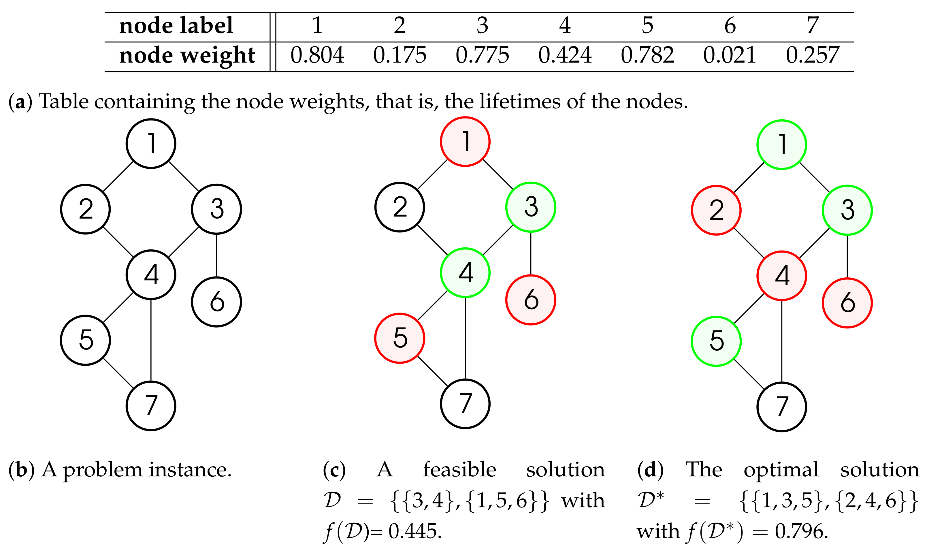
Illustrative Example

Figure 1 provides an illustrative example of the MWDDS problem. Figure 1a,b provide a problem instance and the lifetime values of the nodes in terms of node weights, respectively. Note that, for the sake of simplicity, the lifetime values are normalized between 0 and 1. Figure 1c shows a feasible solution $\mathcal{D}:=\{D_1=\{3,4\},D_2=\{1,5,6\}\}$, that is, solution D contains the two dominating sets $D_1=\{3,4\}$ and $D_2=\{1,5,6\}$. The lifetimes of nodes 3 and 4 are 0.775 and 0.424, respectively. Therefore, the lifetime of $D_1$ is 0.424. Moreover, the lifetimes of nodes 1, 5, and 6 are 0.804, 0.782 and 0.021, respectively. This means that the lifetime of $D_2$ is 0.021. As a consequence, the objective function value $f\left(D\right)$ of D is the sum of 0.424 and 0.021, which results in 0.445. In contrast, Figure 1d shows the optimal solution to this problem instance, that is, ${\mathcal{D}}^{*}:=\{D_1=\{1,3,5\},D_2=\{2,4,6\}\}$. According to the lifetime values of the single nodes, the lifetime of $D_1$ is 0.775, while the lifetime value of $D_2$ is 0.021. Therefore, the objective function value $f\left({\mathcal{D}}^{*}\right)$ of ${\mathcal{D}}^{*}$ is 0.796. Finally, note that, since this graph contains a node of degree 1, any valid solution contains at most two disjoint dominating sets.

3. An ILP Model for the MWDDS Problem

Our ILP model for the MWDDS problem requires the following sets of variables. First, we introduce a binary variable $x_{ij}$ for each node $v_i$ ($i=1,\dots ,n$) and each possible disjoint set $D_j$ ($j=1,\dots ,\delta \left(G\right)+1$). Hereby, $\delta \left(G\right):=min\left\{deg\right(v)\mid v\in V\}$. (Remember that the maximum number of disjoint dominating sets in a graph is $\delta \left(G\right)+1$.) When $x_{ij}=1$, node $v_i$ is assigned to the $j$-th dominating set. Second, a binary variable $y_j$ ($j=1,\dots ,\delta \left(G\right)+1$) indicates whether or not the $j$-th set is opened. Finally, a real-valued variable $z_j\in [0,M]$ ($M\in {\mathbb{R}}^{+}$) stores the weight of the $j$-th dominating set. Hereby, $M:=max\left\{\mathit{lifetime}\right(v)\mid v\in V\}$. Based on these variables, the MWDDS can be stated as an ILP in the following way.

$$\begin{array}{ccc}\hfill \mathbf{max}& \sum _{j=1}^{\delta \left(G\right)+1}{z}_j\hfill & \end{array}$$

(5)

$$\begin{array}{ccc}\hfill \mathbf{s}.\mathbf{t}.& \sum _{j=1}^{\delta \left(G\right)+1}{x}_{ij}\le 1\hspace{1em}\hspace{1em}\hspace{1em}\hspace{1em}\hspace{1em}\hspace{1em}\hspace{1em}\hfill & \hfill i=1,\dots ,n\end{array}$$

(6)

$$\begin{array}{ccc}\hfill & \sum _{v_k\in N\left(v_i\right)}{x}_{kj}\ge y_j-x_{ij}\hspace{1em}\hspace{1em}\hspace{1em}\hspace{1em}\hspace{1em}\hspace{1em}\hspace{1em}\hfill & \hfill j=1,\dots ,\delta \left(G\right)+1\end{array}$$

(7)

$$\begin{array}{ccc}\hfill & y_j\ge x_{ij}\hspace{1em}\hspace{1em}\hspace{1em}\hspace{1em}\hspace{1em}\hspace{1em}\hspace{1em}\hfill & \hfill i=1,\dots ,n and j=1,\dots ,\delta \left(G\right)+1\end{array}$$

(8)

$$\begin{array}{ccc}\hfill & x_{ij}·\mathit{lifetime}\left(v_i\right)+(1-x_{ij})·M\ge z_j\hspace{1em}\hspace{1em}\hfill & \hfill i=1,\dots ,n and j=1,\dots ,\delta \left(G\right)+1\end{array}$$

(9)

$$\begin{array}{ccc}\hfill & y_j·M\ge z_j\hspace{1em}\hspace{1em}\hspace{1em}\hspace{1em}\hspace{1em}\hspace{1em}\hspace{1em}\hfill & \hfill j=1,\dots ,\delta \left(G\right)+1\end{array}$$

(10)

$$\begin{array}{ccc}\hfill & y_j\ge y_{j+1}\hspace{1em}\hspace{1em}\hspace{1em}\hspace{1em}\hspace{1em}\hspace{1em}\hspace{1em}\hspace{1em}\hfill & \hfill j=1,\dots ,\delta \left(G\right)\end{array}$$

(11)

$$\begin{array}{ccc}\hfill & z_j\ge z_{j+1}\hspace{1em}\hspace{1em}\hspace{1em}\hspace{1em}\hspace{1em}\hspace{1em}\hspace{1em}\hspace{1em}\hfill & \hfill j=1,\dots ,\delta \left(G\right)\end{array}$$

(12)

The objective function sums over the weight values of all dominating sets. Note that, for this objective function to be correct, the weight value of those dominating sets that are not opened must be set to zero by respective constraints. Constraints (6) require that each node of the graph is assigned to at most one dominating set. This assures the disjointness of the dominating sets. Next, constraints (7) are the so-called dominating set constraints, that is, they ensure that, if the $j$-th set is opened, then the set of nodes assigned to the j-th set form a dominating set of G. Further, constraints (8) make sure that nodes can only be assigned to opened dominating sets. Constraints (9) are responsible for correctly determining the weights of the opened dominating sets. In other words, the value of variable $z_j$ of the $j$-th dominating set (if open) is set to the minimum of the lifetime-values of all nodes assigned to this set. Next, constraints (10) ensure that the weight values of dominating sets that are not opened are set to zero. Finally, the last two sets of constraints—that is, constraints (11) and (12)—are not necessary for the correctness of the ILP. They are tie-breaking constraints that ensure that (1) if k dominating sets are opened, they are assigned to sets $1,\dots ,k$ and (2) the opened dominating sets are ordered according to a non-increasing weight value.

4. Proposed Greedy Heuristic

Greedy algorithms are constructive heuristics for building feasible solutions to combinatorial optimization problems. They start from an empty solution and iteratively add the most favorable component from a set of feasible extensions of the current partial solution until a complete solution is reached. That is, the component to be added at each construction step is chosen deterministically according to some greedy function, which is a measure for the goodness of the solution components. In general, greedy heuristics do not require overly large computation times. The main drawback of a greedy heuristic is that the single constructed solution is most likely not optimal.

The pseudo-code of our greedy algorithm, henceforth labelled GH-MWDDS, is presented in Algorithm 1. Note that our greedy algorithm is a centralized algorithm which must be executed on a central unit that has the knowledge about the topology of the network and about the lifetime values of the individual nodes. At the start of the algorithm, the following sets are initialized. Solution $\mathcal{D}$ is initialized to the empty set. Furthermore, set $V_{\mathrm{rem}}$, which contains all nodes that may still be added to a dominating set, is initialized to V. Finally, set $V_{\mathrm{done}}$, which collects all nodes that already form part of a dominating set in $\mathcal{D}$, is initialized to the empty set. Counter k counts the number of dominating sets that are being constructed. It is initialized to zero. At each main iteration $k\ge 1$, the algorithm generates a dominating set $D_k$ consisting of nodes from set $V_{\mathrm{rem}}$ which, as mentioned above, contains all nodes of G that do not form part of any of the already generated dominating sets $D_i$, $i=1,\dots ,k-1$; see lines 5 and 21. The algorithm stops once no further dominating set can be generated from the nodes in $V_{\mathrm{rem}}$. This is the case if at least one node $v\in V$ and all its neighbors form part of $V_{\mathrm{done}}$. More formally, the algorithm stops if there is at least one $v\in V$ such that $N\left[v\right]$ is a subset of $V_{\mathrm{done}}$ (see line 5).

Algorithm 1 GH-MWDDS: A Greedy heuristic for the MWDDS problem

Input:  a simple, node-weighted, undirected graph $G=(V,E,\mathit{lifetime})$ Output:  a family of disjoint dominating sets $\mathcal{D}=\{D_1,D_2,\cdots ,D_k\}$ 1: $\mathcal{D}\leftarrow \varnothing$ 2: $k\leftarrow$ 0 3: $V_{\mathrm{rem}}\leftarrow V$ 4: $V_{\mathrm{done}}\leftarrow \varnothing$ 5: while not exists $v\in V$ s.t. $N\left[v\right]$ is a subset of $V_{\mathrm{done}}$ do 6:  $k\leftarrow k+1$ 7:  for each node $v\in V$ do 8:     $color\left(v\right)\leftarrow$ WHITE 9:  end for 10:   $D_k\leftarrow \varnothing$ 11:   while$D_k$ is not a dominating set of G (that is, $N\left[D_k\right]\ne V$) do 12:      $v^{*}\leftarrow \mathrm{argmax}\{score\left(v\right)\mid v\in \{\mathcal{G}\left(D_k\right)\cup \mathcal{W}\left(D_k\right)\}\cap V_{\mathrm{rem}}\}$ 13:      $D_k\leftarrow D_k\cup \left\{v^{*}\right\}$ 14:      $V_{\mathrm{rem}}\leftarrow V_{\mathrm{rem}}\setminus \left\{v^{*}\right\}$ 15:      for each node $u\in N\left(v^{*}\right)$ do 16:        if ( $color\left(u\right)=$ WHITE ) then 17:           $color\left(v\right)\leftarrow$ GRAY 18:        end if 19:    end for 20:    $color\left(v^{*}\right)\leftarrow$ BLACK 21:   end while 22:   Reduce($D_k$, $V_{\mathrm{rem}}$, $V_{\mathrm{done}}$) {optional} 23:   $\mathcal{D}\leftarrow \mathcal{D}\cup \left\{D_k\right\}$ 24:   $V_{\mathrm{done}}\leftarrow V_{\mathrm{done}}\cup D_k$ 25: end while 26: return$\mathcal{D}=\{D_1,D_2,\cdots ,D_k\}$.

The construction of a dominating set $D_k$ at round k of the algorithm is done as follows. First, $D_k$ is initialized to the empty set. At each moment, each node of the input graph G belongs to one of the following sets:

• Black nodes: Nodes that are part of $D_k$.
• Gray nodes: Nodes in $\mathcal{G}\left(D_k\right):=N\left(D_k\right)\setminus D_k$, that is, nodes that are not contained in $D_k$ but that are adjacent to at least one black node.
• White nodes: Nodes in $\mathcal{W}\left(D_k\right):=V\setminus N\left[D_k\right]$, that is, nodes that are neither gray nor black.

Remember, in this context, that $N\left(D_k\right)$ and $N\left[D_k\right]$ denote the open neighborhood and the closed neighborhood of $D_k$, respectively. Given these definitions, $D_k$ is iteratively generated by adding at each construction step exactly one node from $\{\mathcal{G}\left(D_k\right)\cup \mathcal{W}\left(D_k\right)\}\cap V_{\mathrm{rem}}$, that is, a nodes that is (1) either gray or white, and (2) that is not already added to one of the dominating sets from previous rounds. In order to make this choice, all nodes from $\{\mathcal{G}\left(D_k\right)\cup \mathcal{W}\left(D_k\right)\}\cap V_{\mathrm{rem}}$ are evaluated by means of greedy function $score\left(\right)$, which is defined as follows:

$$\begin{array}{cccc}\hfill & score\left(v\right):=\mathit{lifetime}\left(v\right)*white\_degree\left(v\right)\hspace{1em}\hfill & \hfill \forall v\in \{\mathcal{G}\left(D_k\right)\cup \mathcal{W}\left(D_k\right)\}\cap V_{\mathrm{rem}}& \hfill \end{array}$$

(13)

$$\begin{array}{ccc}\hfill & white\_degree\left(v\right):=|N\left[v\right]\cap \mathcal{W}\left(D_k\right)|\hfill & \hfill \end{array}$$

(14)

In other words, the greedy function of a node v is obtained by multiplying the lifetime of the node with the number of white nodes from the closed neighborhood of v.

To further improve the quality of solutions, the dominating set $D_k$ might be reduced by removing redudant nodes before adding $D_k$ to solution $\mathcal{D}$. This is done in the optional function Reduce$(D_k,V_{\mathrm{rem}},V_{\mathrm{done}})$; see line 22 of the pseudo-code. Formally, a node $v\in D_k$ is redundant if each node from its closed neighborhood $N\left[v\right]$ is dominated by at least two nodes from $D_k$, that is, $N\left[v\right]\subset {\bigcup }_{u\in D_k\setminus \left\{v\right\}}N\left[u\right]$ [25]. Redundant nodes are identified and removed in an iterative way. Moreover, sets $V_{\mathrm{rem}}$ and $V_{\mathrm{done}}$ are updated accordingly.

Time Complexity of GH-MWDDS

In this section, we analyze the complexity of our greedy algorithm, without the optional reduction mechanism from line 22. The main while loop (line 5) of the algorithm is iterated k times (rounds), where k refers to the number of disjoint dominating sets returned by the algorithm. Since the maximum number of dominating sets in a domatic partition of a graph $G=(V,E)$ is less or equal to $\delta +1$ [19], where $\delta$ is the minimum degree of any node of G, it holds that $k\le \delta +1$. As a result, checking the condition in line 5 and executing lines 7-9 is both done in $O(\delta ·n)$ time. Further, n is clearly an upper bound for the number of times that the inner while loop (lines 11-21) is iterated. To determine the time complexity of line 12, we proceed as follows. Remember that for any node v the calculation of its $white\_degree\left(v\right)$ value requires $deg\left(v\right)$ operations. Moreover, for choosing the first node $v_1^{*}$ of a dominating set, line 12 requires a time of $deg\left(v_1\right)+deg\left(v_2\right)+\cdots +deg\left(v_n\right)$. The well-known Handshaking Lemma states that ${\displaystyle \sum _{v\in V}}deg\left(v\right)=2m$, where $m=\left|E\right|$. For choosing the second node $v_2^{*}$, line 12 requires $m-deg\left(v_1^{*}\right)$ time, etc. Therefore, the total time complexity of line 12 is $O\left(nm\right)$. In summary, we can conclude that our greedy algorithm has a worst-case time complexity of $O\left(\delta n\right)+O\left(nm\right)=O\left(max\right(\delta n,nm\left)\right)=O\left(nm\right)$.

5. Experimental Evaluation

The proposed greedy algorithm (GH-MWDDS) was implemented in ANSI C++ using GCC 7.4.0 for compiling the software. Its performance was compared with three recent local search approaches available from the related literature [23]: Local Search (LS), Fixed Depth (FD), and Variable Depth (VD). In order to conduct a fair comparison to the three local search algorithms (LS, FD and VD) we used the original source code provided by the authors of [23]. GH-MWDDS and the three local search algorithms were experimentally evaluated on a laptop equipped with a 64-bit 2.5-GHz Intel^® Core™ i5-7200U processor and 8 GB of RAM. We applied GH-MWDDS to a set of 640 problem instances that are described below. Moreover, in order to test the usefulness of our ILP model, we applied the ILP solver ILOG CPLEX 20.01 in single-threaded mode to all problem instances. The time limit for each application of CPLEX was set to 2 CPU hours. Moreover, the experiments with CPLEX were performed on a cluster of machines with two Intel^® Xeon^® Silver 4210 CPUs with 10 cores of 2.20 GHz and 92 Gbytes of RAM.

5.1. Problem Instances

We used the source code provided in [23] for generating 640 diverse problem instances. Each problem instance was generated according to two control parameters: The size of the network n (number of nodes) and its average degree d, where $d=2m/n$ and m is the number of edges. More specifically, we considered five different network sizes: 50, 100, 150, 200 and 250 nodes. For each network size, we considered between 5 to 8 different average degrees in a way such that networks over a range from sparse to dense networks are generated. In addition, each node (sensor) of the network was given a random real value between 0 and 1 as node weight (lifetime). Then, for each combination of n and d, 20 different networks were randomly generated resulting in a total of 640 problem instances for the experimental evaluation.

5.2. Results and Discussion

Table 1. Numerical results of comparison between LS, FD, VD and GH-MWDDS.

n	d	CPLEX		LS		FD		VD		|DP|	GH-MWDDS
		Value	Gap(%)	Value	Time(s)	Value	Time(s)	Value	Time(s)		Value	Time(s)	|DP|
50	15	2.779	32.839	0.395	0.003	0.477	0.019	0.555	1.984	2.55	2.155	0.000	5.75
	20	3.922	121.088	0.649	0.004	0.825	0.055	1.014	7.651	3.55	3.353	0.001	8.05
	25	5.098	158.038	1.011	0.006	1.245	0.055	1.490	4.885	4.05	4.595	0.001	10.05
	30	6.432	200.567	1.664	0.007	2.460	0.124	2.780	13.117	6.30	5.926	0.001	12.90
	35	7.929	197.434	2.200	0.012	2.914	0.204	3.166	25.048	6.85	7.376	0.000	15.30
100	20	2.467	405.669	0.283	0.023	0.333	0.188	0.423	30.458	2.45	2.784	0.001	7.00
	30	3.202	>1000.0	0.431	0.017	0.535	0.165	0.576	31.796	2.95	4.501	0.003	10.90
	40	3.338	>1000.0	0.859	0.021	1.259	0.394	1.341	183.921	4.75	6.679	0.002	14.80
	50	3.857	>1000.0	1.361	0.038	2.018	0.796	2.407	225.704	6.00	8.500	0.001	18.65
	60	5.804	823.022	2.019	0.027	2.884	0.830	3.226	362.775	7.15	11.131	0.001	23.40
150	30	0.055	>1000.0	0.287	0.053	0.326	0.316	0.326	106.602	2.85	4.098	0.002	10.65
	40	0.028	>1000.0	0.557	0.050	0.670	0.595	0.745	156.994	3.80	5.816	0.003	14.05
	50	0.011	>1000.0	0.615	0.077	0.927	1.139	1.009	182.630	3.95	7.479	0.003	17.50
	60	0	>1000.0	0.848	0.046	1.506	2.576	1.521	646.268	4.90	9.281	0.002	21.00
	70	0	>1000.0	1.373	0.066	2.293	4.219	2.464	1028.650	6.65	11.388	0.004	24.45
	80	0	>1000.0	1.689	0.065	2.729	2.599	3.036	549.900	7.20	13.508	0.005	28.90
	90	0	>1000.0	2.209	0.055	3.817	3.793	4.193	906.030	9.05	15.485	0.006	32.95
200	40	0	>1000.0	0.256	0.049	0.317	0.648	0.370	81.750	2.65	5.424	0.004	13.65
	50	0	>1000.0	0.374	0.099	0.475	1.252	0.483	186.900	3.45	6.784	0.005	16.60
	60	0	>1000.0	0.678	0.112	0.897	2.083	0.917	313.850	3.75	8.656	0.005	20.35
	70	0	>1000.0	1.004	0.170	1.652	6.463	1.680	3112.950	5.95	10.351	0.006	23.65
	80	0	>1000.0	0.840	0.076	1.624	5.874	1.795	1629.400	5.35	12.447	0.008	27.15
	90	0	>1000.0	1.153	0.109	1.924	5.260	2.045	1364.400	5.65	13.978	0.012	30.55
	100	0	>1000.0	1.503	0.091	2.836	9.396	3.098	3024.830	7.65	15.868	0.009	34.30
250	50	0	>1000.0	0.266	0.136	0.314	0.867	0.329	557.676	2.95	6.681	0.016	16.85
	60	0	>1000.0	0.526	0.221	0.892	7.638	0.945	1400.788	4.55	8.244	0.012	19.70
	70	0	>1000.0	0.689	0.264	1.050	6.906	1.326	2380.366	5.10	9.636	0.013	22.95
	80	0	>1000.0	0.652	0.241	1.163	9.801	1.445	647.763	5.40	11.520	0.013	26.15
	90	0	>1000.0	0.841	0.324	1.448	18.394	1.591	1242.663	5.80	12.938	0.013	29.55
	100	0	>1000.0	1.117	0.228	1.981	20.789	2.443	2210.880	6.45	14.733	0.016	32.70
	120	0	>1000.0	1.259	0.146	2.577	10.442	2.781	2249.350	7.20	18.348	0.016	39.70
	140	0	>1000.0	2.135	0.121	4.275	16.885	4.713	6624.596	10.50	22.478	0.020	47.25
Avg		1.404		0.992	0.092	1.583	4.399	1.757	984.143	5.231	9.442	0.006	21.169

reports on the performance comparison of GH-MWDDS (without the optional reduction procedure) and LS, FD, VD, and CPLEX. The first two columns indicate the problem instance type. More specifically, the number of nodes (n) is provided in the first column, whereas the average degree (d) is shown in the second column. Obviously, the higher d, the more dense is the network. Remember that for each combination of n and d—that is, for each table row—there are 20 randomly generated problem instances. The values shown in the tables represent the average results obtained for these 20 instances per table row. Table columns 3 and 4 contain the results of CPLEX. While the first one of these columns indicates the average solution quality obtained, the second column provides the average gap (in percent) between the found results and the upper bounds. The results of the other algorithms are provided in two columns for each algorithm. These columns report on the average solution quality (Value) and the average computation time (Time(s)) in seconds. Moreover, the 11-th column of the table indicates the average size of solutions ($\left|DP\right|$) in terms of the average number of disjoint dominating sets. Since the three algorithms LS, FD and VD start with the same greedy solution as initial solution, and the number of disjoint dominating sets does not change during local search, the column with heading $\left|DP\right|$ holds for all three algorithms. Finally, in the last column of the table, the average size of the solutions of GH-MWDDS is given.

In addition to evaluating GH-MWDDS, we also tested the following two additional versions. Henceforth we refer to the version of GH-MWDDS that removes redundant nodes in line 22 as GH-MWDDS${}^{+}$. In addition, the algorithm can be easily adapted in order to solve the maximum disjoint dominating sets (MDDS) problem, instead of the MWDDS. The resulting greedy algorithm, which is called GH-MDDS, is obtained by replacing the $score(·)$ function in line 12 of Algorithm 1 by the $white\_degree(·)$ function of Equation (14). The experiential results obtained with GH-MDDS and GH-MWDDS${}^{+}$ are provided in

Table 2. Numerical results of comparison between GH-MDDS, GH-MWDDS and GH-MWDDS${}^{+}$.

n	d	GH-MDDS			GH-MWDDS			GH-MWDDS${}^{+}$
		Value	Time(s)	|DP|	Value	Time(s)	|DP|	Value	Time(s)	|DP|
50	15	1.111	0.001	6.75	2.155	0.000	5.75	2.191	0.002	6.150
	20	1.548	0.001	9.05	3.353	0.001	8.05	3.450	0.000	8.350
	25	2.630	0.001	11.85	4.595	0.001	10.05	4.672	0.000	10.550
	30	3.510	0.001	14.60	5.926	0.001	12.90	6.042	0.000	13.350
	35	4.772	0.001	17.25	7.376	0.000	15.30	7.546	0.000	15.900
100	20	0.841	0.001	8.50	2.784	0.001	7.00	2.842	0.001	7.400
	30	1.714	0.004	12.70	4.501	0.003	10.90	4.580	0.001	11.150
	40	2.900	0.002	17.15	6.679	0.002	14.80	6.794	0.002	15.200
	50	3.908	0.002	21.40	8.500	0.001	18.65	8.525	0.002	19.100
	60	6.111	0.004	26.30	11.131	0.001	23.40	11.174	0.002	23.600
150	30	1.036	0.003	12.00	4.098	0.002	10.65	4.141	0.002	10.900
	40	1.769	0.002	16.20	5.816	0.003	14.05	5.872	0.002	14.350
	50	2.553	0.003	20.00	7.479	0.003	17.50	7.570	0.002	17.850
	60	3.647	0.004	24.10	9.281	0.002	21.00	9.371	0.005	21.450
	70	4.789	0.002	28.10	11.388	0.004	24.45	11.446	0.005	25.050
	80	6.468	0.005	33.00	13.508	0.005	28.90	13.611	0.003	29.150
	90	7.143	0.006	36.55	15.485	0.006	32.95	15.589	0.005	33.550
200	40	1.350	0.006	15.50	5.424	0.004	13.65	5.486	0.005	13.950
	50	1.719	0.006	18.95	6.784	0.005	16.60	6.848	0.006	17.050
	60	2.551	0.007	23.35	8.656	0.005	20.35	8.710	0.008	20.550
	70	3.566	0.008	26.80	10.351	0.006	23.65	10.395	0.008	24.100
	80	4.466	0.015	30.70	12.447	0.008	27.15	12.529	0.003	27.400
	90	5.368	0.009	34.80	13.978	0.012	30.55	14.046	0.009	31.000
	100	6.425	0.011	38.50	15.868	0.009	34.30	15.993	0.009	34.650
250	50	1.643	0.013	19.05	6.681	0.016	16.85	6.783	0.008	16.950
	60	2.062	0.010	22.70	8.244	0.012	19.70	8.285	0.010	19.950
	70	2.613	0.012	26.15	9.636	0.013	22.95	9.699	0.013	23.150
	80	3.348	0.013	29.55	11.520	0.013	26.15	11.571	0.013	26.500
	90	4.030	0.016	33.50	12.938	0.013	29.55	12.978	0.016	29.900
	100	5.024	0.016	37.15	14.733	0.016	32.70	14.800	0.016	33.150
	120	7.134	0.017	45.05	18.348	0.016	39.70	18.418	0.018	40.250
	140	9.584	0.020	53.60	22.478	0.020	47.25	22.514	0.020	47.700
Avg		3.667	0.007	24.089	9.442	0.006	21.169	9.515	0.006	21.541

, whose structure is very similar to the one of Table 1.

From the results displayed in Table 1 and Table 2, the following observations can me made:

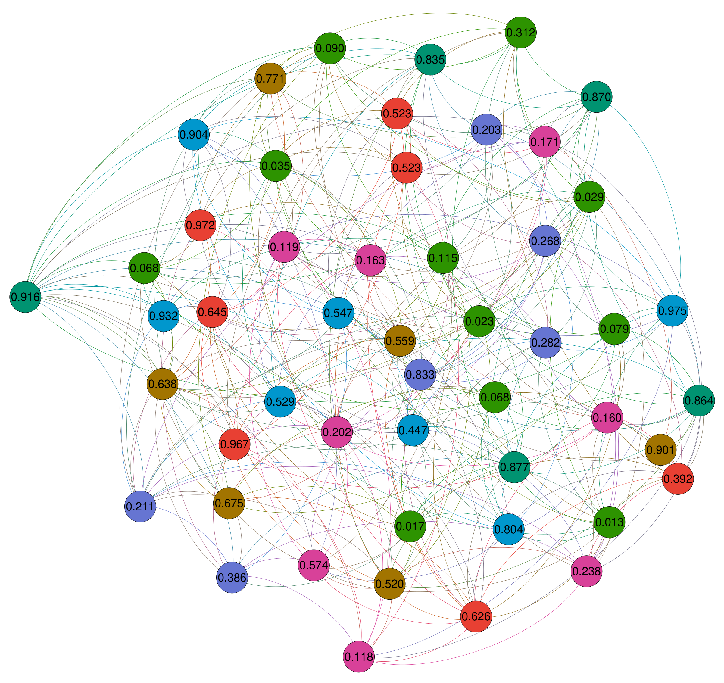
• First of all, the ILP model (solved by CPLEX) is only useful in the context of the smallest problem instances. In fact, CPLEX obtains the best results for all networks with 50 nodes. As an additional information we can say that CPLEX was able to solve 8 out of 20 problem instances with 50 nodes and an average degree of 15 to optimality. Figure 2 exemplary shows the optimal solution obtained by CPLEX for network number 14 of those networks with 50 nodes and an average node degree of 15. Note that the nodes are divided into six dominating sets (as indicated by the colors of the nodes). The nodes which are colored in green are not assigned to any dominating set.
• CPLEX already starts to fail for the instances with 100 nodes, for which the results are already inferior to those of GH-MWDDS. In fact, for most of the problem instances (starting from 150 nodes and an average degree of 60) CPLEX is unable to find anything but the trivial solution that contains no dominating set.
• Concerning GH-MWDDS, we can observe that it dominates the three competitors from the literature for all problem instances in terms of solution quality as well as computational time. It is significantly better than the best of the other three approaches, while requiring a computation time that is approximately five orders of magnitude smaller than the time needed by the other methods. The improvement ratio of our algorithm with respect to VD (the best approach from the literature) is about 5.37.
• As expected, most solutions suffer from the existence of redundant nodes. As a result, GH-MWDDS${}^{+}$ is able to produce solutions whose size (in terms of the number of disjoint dominating sets) is increased with respect to the solutions produced by GH-MWDDS. This is achieved without compromising the quality of the generated solutions. On the contrary, the quality of the obtained solutions is slightly improved, at the cost of a negligible amount of computation time.
• In addition, from Table 2 we can observe that GH-MDDS and GH-MWDDS${}^{+}$ achieve an overall average solution quality (see that last row of Table 2) of 3.667 and 9.515, respectively, and an average solution size (in terms of the number of disjoint dominating sets) of 24.089 and 21.541, respectively. It is worthwhile to note that GH-MDDS always produces solutions with the maximum possible size (equal to $\delta \left(G\right)+1$). However, the quality of these solutions (as measured by the objective function of the MWDDS problem) is, of course, lower than the quality of the solutions produced by GH-MWDDS. This is because GH-MDDS is primarily focused on finding solutions of large size, without taking into consideration the problem-specific knowledge of the lifetime values of the nodes. Therefore, a solution to the MWDDS problem with the maximum size does not necessarily correspond to the best MWDDS-solution. For example, in the case where n = 250 and d = 140, for which GA-MDDS finds a solution with an average value 9.584 and an average size 53.6, GH-MWDDS${}^{+}$ finds solutions with an average value 22.514 and average size 47.7.
• From above observations we can say that the poor performance of the three local search algorithms proposed by Pino et al. [23] is mainly due to greedy heuristic used for producing the initial solutions for their local search approaches. Since this greedy heuristic was developed for the MDDS problem, and the local search approaches try to improve these solutions by making swaps among nodes of different disjoint dominating sets, they are limited to the size of the solutions found by the initial greedy heuristic, which cannot be changed later. As can be seen by our results, this way of proceeding limits too much the possibility of the local search algorithms to find improvements.

In summary we can say that our GH-MWDDS approach is clearly a new state-of-the-art method for the MWDDS problem. In order to study the scalability of our approach, we finally generated two large-scale random geometric graphs with 10,000 nodes. Both graphs were generated by scattering 10,000 nodes randomly in the unit square, and connecting each pair of nodes whose geometric distance is below $r=0.02$ (first graph), respectively $r=0.03$ (second graph). The first graph has 61,646 edges, while the second one has 137,317 edges. The computation time of GH-MWDDS was 1.829 seconds for the first graph and 5.054 seconds for the second graph. This difference in computation time between the first and the second graph is due to the different density, which leads to a solution with two dominating sets in the case of the first graph and a solution with six dominating sets in the case of the second graph. The important point, however, is that the computation time of our algorithm is still very low, even in the context of large-scale graphs. The solutions of GH-MWDDS are graphically shown in Figure 3. Note that, in the case of the first graph, red and green nodes form dominating sets, while all but the pink-colored nodes in the case of the second graph are assigned to six different dominating sets.

6. Conclusions

This paper deals with the network lifetime maximization problem using the approach of computing disjoint dominating sets in a given network in which sensors are characterized by different lifetime values. In other words, we considered a version of the weighted disjoint dominating sets problem. In this context, we have proposed a greedy heuristic that benefits from the use of problem-specific knowledge. To assess the performance of our algorithm, 640 problem instances of different sizes (both sparse and dense graphs) were evaluated and the obtained results were compared with those of three recently published local search algorithms. Computational results show the superiority of our greedy algorithm over recent approaches available from the literature. In addition, we stated the considered problem as an integer linear programming model. However, the results of applying CPLEX to solve the model have shown that this approach is only useful for the smallest ones of the considered networks.

Finally, note that our approach can directly be applied to disconnected graphs, that is, our implementation considers the possible existence of disconnected sub-graphs. Moreover, the approach can easily be adapted to directed graphs. The only aspect that has to change for the application to directed graphs is the definition of a dominating set (see, for example, [26]) and the way in which such dominating sets are generated at each main loop of the greedy heuristic.

In the future we plan to develop well-working metaheuristics on the basis of the developed greedy heuristic in order to further improve the obtained results. Options include ant colony optimization or iterated greedy algorithms, which are both based on the step-by-step construction of solutions. Another line of research will focus on hybrid techniques such as construct, merge, solve and adapt (CMSA) [27], which make it possible to take profit from ILP solvers such as CPLEX even in the context of instances of large problem.

References

1. Yetgin, H.; Cheung, K.T.K.; El-Hajjar, M.; Hanzo, L.H. A survey of network lifetime maximization techniques in wireless sensor networks. IEEE Commun. Surv. Tutor. 2017, 19, 828–854. [Google Scholar] [CrossRef] [Green Version]
2. Rodrigues, L.M.; Montez, C.; Budke, G.; Vasques, F.; Portugal, P. Estimating the lifetime of wireless sensor network nodes through the use of embedded analytical battery models. J. Sens. Actuator Netw. 2017, 6, 8. [Google Scholar] [CrossRef] [Green Version]
3. Lewandowski, M.; Płaczek, B.; Bernas, M. Classifier-Based Data Transmission Reduction in Wearable Sensor Network for Human Activity Monitoring. Sensors 2021, 21, 85. [Google Scholar] [CrossRef] [PubMed]
4. Sharma, H.; Haque, A.; Jaffery, Z.A. Maximization of wireless sensor network lifetime using solar energy harvesting for smart agriculture monitoring. Ad Hoc Netw. 2019, 94, 101966. [Google Scholar] [CrossRef]
5. Lewandowski, M.; Bernas, M.; Loska, P.; Szymała, P.; Płaczek, B. Extending Lifetime of Wireless Sensor Network in Application to Road Traffic Monitoring. In International Conference on Computer Networks; Springer: Berlin/Heidelberg, Germany, 2019; pp. 112–126. [Google Scholar]
6. Mansourkiaie, F.; Ismail, L.S.; Elfouly, T.M.; Ahmed, M.H. Maximizing lifetime in wireless sensor network for structural health monitoring with and without energy harvesting. IEEE Access 2017, 5, 2383–2395. [Google Scholar] [CrossRef]
7. Cardei, M.; Thai, M.T.; Li, Y.; Wu, W. Energy-efficient target coverage in wireless sensor networks. In Proceedings of the IEEE 24th Annual Joint Conference of the IEEE Computer and Communications Societies, Miami, FL, USA, 13–17 March 2005; Volume 3, pp. 1976–1984. [Google Scholar]
8. Slijepcevic, S.; Potkonjak, M. Power efficient organization of wireless sensor networks. In Proceedings of the ICC 2001—IEEE International Conference on Communications, Helsinki, Finland, 11–14 June 2001; Volume 2, pp. 472–476. [Google Scholar]
9. Wang, H.; Li, Y.; Chang, T.; Chang, S. An effective scheduling algorithm for coverage control in underwater acoustic sensor network. Sensors 2018, 18, 2512. [Google Scholar] [CrossRef] [PubMed] [Green Version]
10. Liao, C.C.; Ting, C.K. A novel integer-coded memetic algorithm for the set k-cover problem in wireless sensor networks. IEEE Trans. Cybern. 2017, 48, 2245–2258. [Google Scholar] [CrossRef] [PubMed]
11. Chen, Z.; Li, S.; Yue, W. Memetic algorithm-based multi-objective coverage optimization for wireless sensor networks. Sensors 2014, 14, 20500–20518. [Google Scholar] [CrossRef] [PubMed] [Green Version]
12. Balaji, S.; Anitha, M.; Rekha, D.; Arivudainambi, D. Energy efficient target coverage for a wireless sensor network. Measurement 2020, 165, 108167. [Google Scholar] [CrossRef]
13. D’Ambrosio, C.; Iossa, A.; Laureana, F.; Palmieri, F. A genetic approach for the maximum network lifetime problem with additional operating time slot constraints. Soft Comput. 2020, 1–7. [Google Scholar] [CrossRef]
14. Li, J.; Potru, R.; Shahrokhi, F. A Performance Study of Some Approximation Algorithms for Computing a Small Dominating Set in a Graph. Algorithms 2020, 13, 339. [Google Scholar] [CrossRef]
15. Li, R.; Hu, S.; Liu, H.; Li, R.; Ouyang, D.; Yin, M. Multi-Start Local Search Algorithm for the Minimum Connected Dominating Set Problems. Mathematics 2019, 7, 1173. [Google Scholar] [CrossRef] [Green Version]
16. Bouamama, S.; Blum, C. An Improved Greedy Heuristic for the Minimum Positive Influence Dominating Set Problem in Social Networks. Algorithms 2021, 14, 79. [Google Scholar] [CrossRef]
17. Garey, M.; Johnson, D. Computers and Intractability. A Guide to the Theory of NP-Completeness; W. H. Freeman: New York, NY, USA, 1979. [Google Scholar]
18. Cardei, M.; MacCallum, D.; Cheng, M.X.; Min, M.; Jia, X.; Li, D.; Du, D.Z. Wireless sensor networks with energy efficient organization. J. Interconnect. Netw. 2002, 3, 213–229. [Google Scholar] [CrossRef]
19. Feige, U.; Halldórsson, M.M.; Kortsarz, G.; Srinivasan, A. Approximating the domatic number. SIAM J. Comput. 2002, 32, 172–195. [Google Scholar] [CrossRef]
20. Moscibroda, T.; Wattenhofer, R. Maximizing the lifetime of dominating sets. In Proceedings of the 19th IEEE International Parallel and Distributed Processing Symposium, Denver, CO, USA, 4–8 April 2005. [Google Scholar]
21. Nguyen, T.N.; Huynh, D.T. Extending sensor networks lifetime through energy efficient organization. In Proceedings of the International Conference on Wireless Algorithms, Systems and Applications (WASA 2007), Chicago, IL, USA, 1–3 August 2007; pp. 205–212. [Google Scholar]
22. Islam, K.; Akl, S.G.; Meijer, H. Maximizing the lifetime of wireless sensor networks through domatic partition. In Proceedings of the 2009 IEEE 34th Conference on Local Computer Networks, Zurich, Switzerland, 20–23 October 2009; pp. 436–442. [Google Scholar]
23. Pino, T.; Choudhury, S.; Al-Turjman, F. Dominating set algorithms for wireless sensor networks survivability. IEEE Access 2018, 6, 17527–17532. [Google Scholar] [CrossRef]
24. Haynes, T.W.; Hedetniemi, S.T.; Henning, M.A. Topics in Domination in Graphs; Springer: Berlin/Heidelberg, Germany, 2020. [Google Scholar]
25. Bouamama, S.; Blum, C. A hybrid algorithmic model for the minimum weight dominating set problem. Simul. Model. Pract. Theory 2016, 64, 57–68. [Google Scholar] [CrossRef]
26. Pang, C.; Zhang, R.; Zhang, Q.; Wang, J. Dominating sets in directed graphs. Inf. Sci. 2010, 180, 3647–3652. [Google Scholar] [CrossRef]
27. Blum, C.; Davidson, P.P.; López-Ibáñez, M.; Lozano, J.A. Construct, Merge, Solve & Adapt: A new general algorithm for combinatorial optimization. Comput. Oper. Res. 2016, 68, 75–88. [Google Scholar]
Figure 1. An illustrative example of the MWDDS problem.
Algorithms 14 00170 g001
Figure 2. An optimal solution for network number 14 with 50 nodes and an average node degree of 15. The solution was produced by CPLEX. The color of the nodes indicates to which of six dominating sets they belong: Blue, dark blue, dark green, red, purple, and brown. The nodes colored in green do not belong to any dominating set.
Algorithms 14 00170 g002
Figure 3. Results of GH-MWDDS for two random geometric graphs of different densities.
Algorithms 14 00170 g003