Abstract
Recently, some researchers adopted the convolutional neural network (CNN) for time series classification (TSC) and have achieved better performance than most hand-crafted methods in the University of California, Riverside (UCR) archive. The secret to the success of the CNN is weight sharing, which is robust to the global translation of the time series. However, global translation invariance is not the only case considered for TSC. Temporal distortion is another common phenomenon besides global translation in time series. The scale and phase changes due to temporal distortion bring significant challenges to TSC, which is out of the scope of conventional CNNs. In this paper, a CNN architecture with an elastic matching mechanism, which is named Elastic Matching CNN (short for EM-CNN), is proposed to address this challenge. Compared with the conventional CNN, EM-CNN allows local time shifting between the time series and convolutional kernels, and a matching matrix is exploited to learn the nonlinear alignment between time series and convolutional kernels of the CNN. Several EM-CNN models are proposed in this paper based on diverse CNN models. The results for 85 UCR datasets demonstrate that the elastic matching mechanism effectively improves CNN performance.
1. Introduction
Time series classification (TSC) is an important research topic in data mining communities [1]. It has a wide range of applications in human activity recognition [2], speech analysis [3], electrocardiogram (ECG) monitoring [4], and biological research [5].
Deep learning is a subfield of machine learning concerned with deep structures with adjustable parameters. Many deep learning architectures exist for TSC. Compared with other classical architectures such as the multilayer perceptron and recurrent neural network (RNN), the convolutional neural network (CNN) has become one of the most prevalent architectures for TSC in recent years [6]. However, the CNN architecture is sensitive to temporal distortion [7], such as differences in rates and local translation within a pattern [8].
Many studies have been conducted on temporal distortion for TSC. One of the most representative studies is on dynamic time warping (DTW). In conjunction with a one-nearest-neighbor (1NN) classifier, DTW achieves great success in TSC. Compared with the lock-step matching in Euclidean distance (ED) [9], elastic matching is exploited in DTW to achieve invariance in temporal distortion. However, DTW is a global distance measure that discards the matching information [8]. In addition, DTW could match two series that have dissimilar local structures [10].
Inspired by the elastic matching in DTW, an elastic matching mechanism combined with CNN called Elastic Matching CNN (EM-CNN) is proposed in this paper. Instead of lock-step alignments between the time series and convolutional kernels as CNN, a matching matrix is used to adaptively learn the alignments between these in the EM-CNN. The EM-CNN is an architecture that learns the matching relationship and convolutional kernel simultaneously. The primary contributions of this paper are concluded as follows:
- An elastic matching mechanism is proposed to measure the similarity between the time series and convolutional kernels. This mechanism can be extended to different architectures based on the CNN.
- The experiments performed on 85 University of California, Riverside (UCR) time series datasets [11] demonstrate that the proposed mechanism improves the performance of CNN on classification tasks.
The remainder of this paper is organized as follows. This paper briefly reviews the related work in Section 2. In Section 3, an elastic matching mechanism is proposed to learn the matching relationship between the time series and convolutional kernels. Next, the experiments are performed on 85 UCR datasets, and the results are analyzed in Section 4. Additional discussion is presented in Section 5. Finally, a conclusion is provided in Section 6.
2. Related Work
2.1. Dynamic Time Warping
Dynamic time warping is a point-to-point matching method to measure the similarity between two different time series. In general, DTW allows a time series to be “stretched” or “compressed” to provide a better match with another time series [12]. Finding a better match in DTW is equivalent to finding an optimal path in the warping matrix with certain restrictions and rules. A dynamic programming algorithm is used to obtain the cumulative distance of the optimal path. A smaller cumulative distance results in a higher similarity between two time series.
The point-to-point matching in DTW is dependent on the value differences between two points. A point of a series could map a further point or multiple points of other series, leading to misclassification, especially in such applications as image retrieval [13]. Constraint techniques, such as Sakoe–Chuba [14] Band and Itakura Parallelogram [15] are introduced to DTW to reduce the matching space. Weighted DTW [12] considers the phase differences besides value differences to penalize the further points which are probably outliers. Derivative DTW [16] and shapeDTW [10] encode the local neighborhood information rather than the values at a point to measure the similarity between two points.
2.2. Dynamic Time Warping with the Convolutional Neural Network
The artificial neural network (ANN) is famous for its powerful feature extraction capability in the last decades. Recently, ANNs such as the RNN and CNN, have been used to learn supervised [17] or unsupervised representation [18] for time series analysis. The RNN is well-known for time series forecasting [17] with the advantage of sequential learning. Some improvements are proposed to reduce inference time [19] and predict sudden time-series changes [20]. Although, the RNN is also exploited in the TSC, the CNN achieves better performance in supervised learning on the UCR archive [21]. The CNN, such as the fully convolutional network (FCN) and residual network (ResNet) [22], have achieved strong baselines for TSC. Some attempts have been made to combine DTW and CNN to overcome the brittleness to temporal distortions in the conventional CNN. These attempts are roughly categorized into two categories. The first category, DTW, is a preprocessing method to transform the raw time series. Then, the transformed series are used as inputs to the CNN. In [8], a multimodal fusion CNN (MMF-CNN) is employed to predict a label for the multidimensional time series. The multidimensional time series are composed of the coordinate features and local distance features which are extracted by measuring the DTW similarity between the original time series and prototypes. The second category directly incorporates the DTW into the CNN and training an end-to-end classification framework. In [23], DTW is used to determine a more optimal alignment between convolutional kernels and time series. The DTWNet [7] replaces the inner product kernel with the DTW kernel against the Doppler effect and improves the capability to do feature extraction.
3. Proposed Method
3.1. Elastic Matching in Dynamic Time Warping
Elastic matching in DTW is first reviewed to better demonstrate the proposed mechanism. Considering two different time series and a dynamic programming algorithm composed of Equations (1) and (2) is used to decide which points should be matched. The second point in X could match the third and fourth points in W (red rhombuses in Figure 1) using DTW. Compared with lock-step matching (blue circles in Figure 1), used in ED, the matching relationship in DTW is data-dependent and elastic:
where is the cumulative distance:
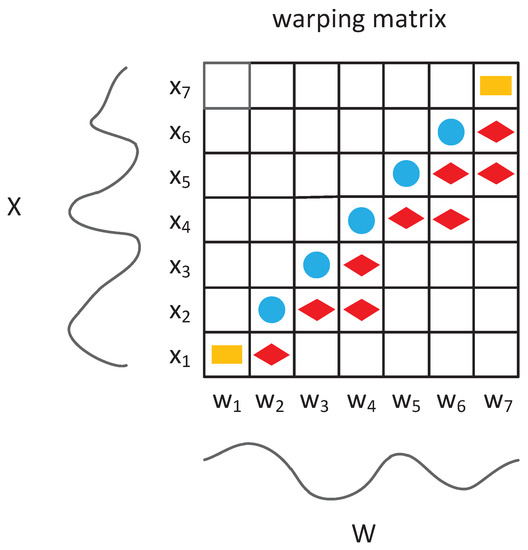
Figure 1.
Example of elastic matching in dynamic time warping (DTW); the yellow rectangles are the beginning and end of the two paths; blue circles and red rhombuses represent the optimal paths in Euclidean distance and DTW, respectively.
3.2. Elastic Matching in the Convolutional Neural Network
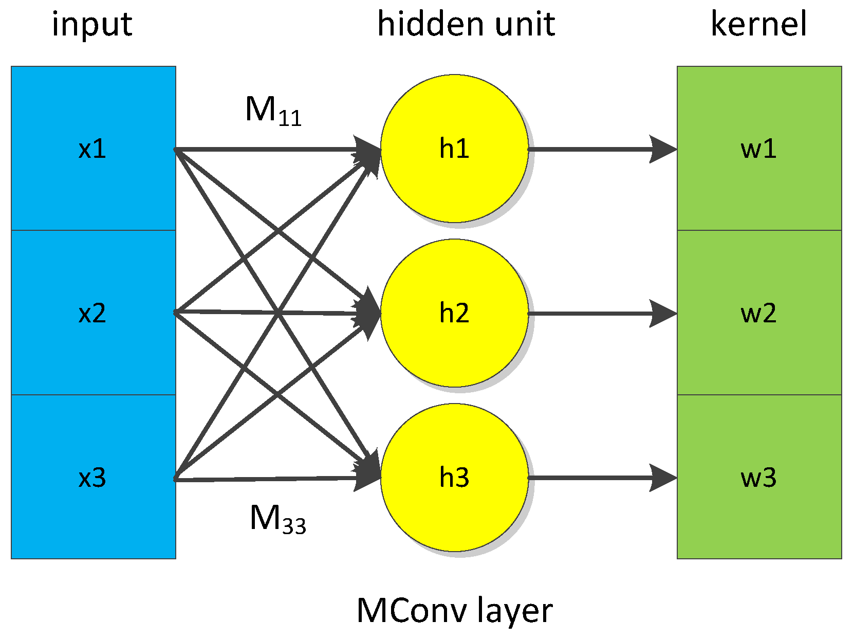
The CNN extracts features from the time series by measuring the local similarity between the time series and convolutional kernel In general, the similarity measure adopted in the CNN is the inner product. Considering the definition of the inner product, the matching mechanism of the inner product is similar to the ED. A point of one series only matches the point of another series in the same position. Hence, the inner product is inappropriate to measure similarity for temporal distortion. An elastic matching mechanism is incorporated into the inner product to better model the matching relationship between the time series and convolutional kernels. The elastic matching mechanism allows the kernel points to construct relationships with points in different positions of the time series. The similarity of the ith location is defined by Equation (3). The convolutional layer combined with the elastic matching mechanism is called the matching convolutional (MConv) layer. The structure of the MConv layer is presented in Figure 2. A fully-connected (FC) layer is used to learn the matching relationship between the series and kernels. The weights of the FC layer in Figure 2 correspond to the matching matrix M in Equation (3).
where m is the length of a convolutional kernel, and M is an matching matrix.

Figure 2.
Structure of the matching convolutional (MConv) layer.
When M is an identity matrix, Equation (3) degenerates to the inner product, and Equation (3) can be considered an extension of DTW. The proof is as follows.
Without loss of generality, this proof is based on the example in Figure 1. The time series and convolutional kernel have the same length in a sliding window for the CNN. Red rhombuses represent the optimal path in Figure 1. Hence, series and kernel are transformed to and as shown in Equation (4), respectively:
If a dot product is used to measure the similarity between two points, the DTW similarity between X and W is equivalent to the inner product between and as presented in Equation (5):
3.3. EM-CNN
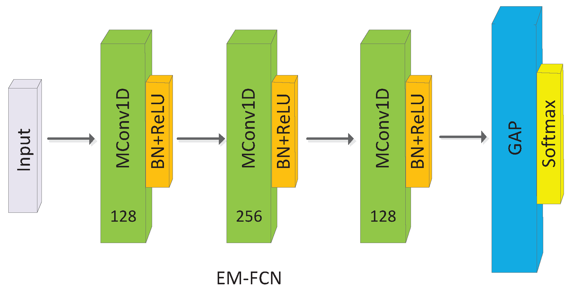
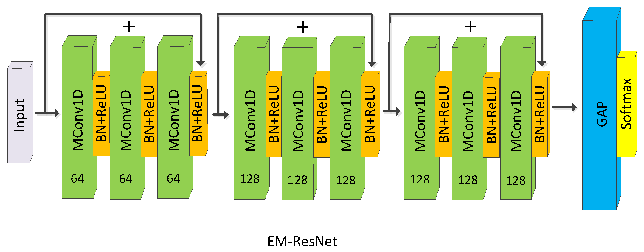
In this section, three EM-CNN architectures including elastic matching FCN (EM-FCN), elastic matching ResNet (EM-ResNet) and elastic matching Inception (EM-Inception) are proposed. The architectures in Figure 3 and Figure 4 are EM-FCN and EM-ResNet. The backbone of the EM-FCN and EM-ResNet are FCN and ResNet which are strong baselines for TSC [22]. The EM-FCN is similar to FCN; the difference between FCN and EM-FCN is the convolutional layers in FCN are replaced by the MConv layers in EM-FCN. The EM-FCN comprises three basic modules, one global average pooling (GAP) layer, and one FC layer. Each basic module contains one MConv layer, one batch normalization (BN) layer, and one Rectified Linear Unit (ReLU) layer. The kernel sizes and numbers of kernels corresponding to the three MConv layers are 8, 5, and 3 and 128, 256, and 128, respectively.
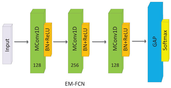
Figure 3.
Architecture of EM-FCN, MConv1D denotes the one-dimensional MConv layer.
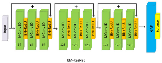
Figure 4.
Architecture of EM-ResNet, MConv1D denotes the one-dimensional MConv layer.
Compared with the EM-FCN, the EM-ResNet is deeper. It has three bottlenecks, which consist of three basic modules like EM-FCN. The number of kernels corresponding to three bottlenecks is 64, 128, and 128, respectively. Convolutional layers are only replaced by MConv layers in the residual branches for stable training.
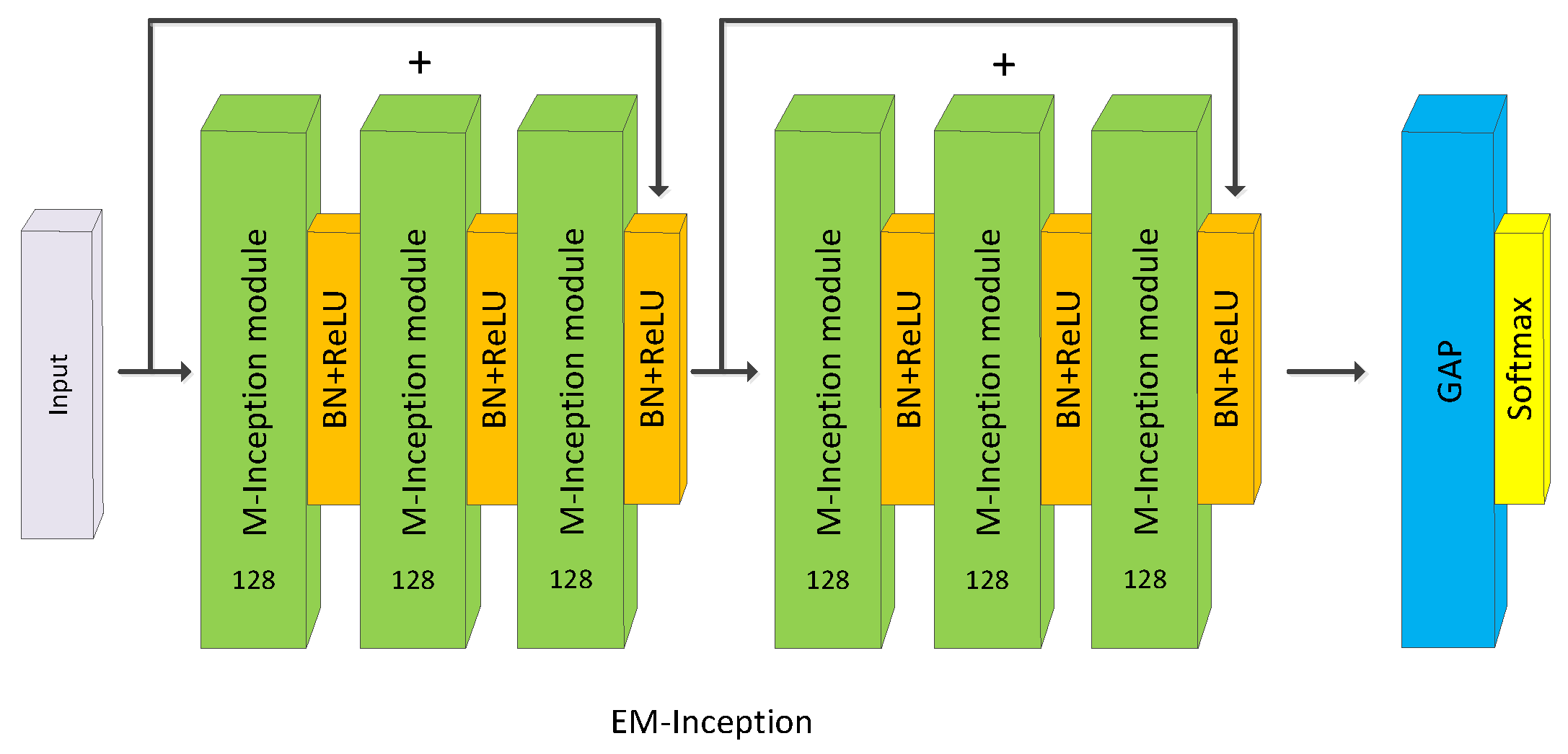
Compared with the EM-FCN and EM-ResNet, EM-Inception (Figure 5) is based on Inception [24] which extracts features in a multiscale manner. Inception is composed of two bottlenecks, one GAP layer, and one FC layer.
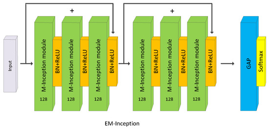
Figure 5.
Architecture of EM-Inception.
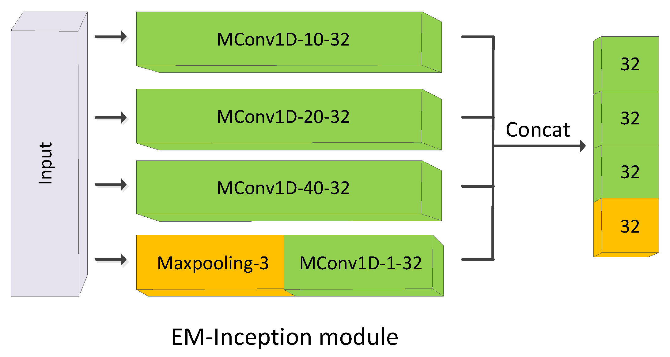
Each bottleneck has three basic Inception modules. Multiple paralleled convolutional operators of different kernel sizes in conjunction with a max-pooling operator are performed in each module in Figure 6. Like EM-ResNet, a shortcut connection is used between the consecutive bottlenecks, and the MConv layers only take the place of the convolutional layers in the residual branches.
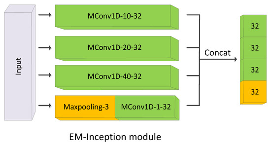
Figure 6.
Architecture of the EM-Inception module, MConv1D denotes the one-dimensional MConv layer. The input of the EM-Inception module is filtered by three Mconv1D with 32 kernels which sizes are 10, 20, and 40, respectively, and one max-pooling layer (stride = 3) followed by a convolutional layer. The output of the EM-Inception module is a feature map with 128 channels.
The MConv layer is the core of the EM-CNN. The matching matrix M in the MConv layer is learned by backpropagation. Similar to the derivation in [25,26], the details for calculating the gradients needed for the backpropagation algorithm are as follows. Figure 2 illustrates that, assuming the response in each location for the MConv layer is y, and the optimized objective function is as follows:
Equation (8) becomes the objective function of CNN if M is an identity matrix. The gradient descent for the CNN is easy to calculate:
4. Experiments
In this section, experiments are performed on the UCR archive to validate the effectiveness of the elastic matching mechanism.
4.1. Hyperparameter Settings
The EM-FCN, EM-ResNet, and EM-Inception were tested on 85 ‘bake-off’ datasets on the UCR archive. Default train/test split was used as [22,24] to train the model and evaluate the performance. The matching matrix M was changed per layer and initialized using an identity matrix. The Adam optimizer was used to train the EM-FCN (2000 epochs), EM-ResNet (1500 epochs) and EM-Inception (1500 epochs) with the initial learning rate of 0.001, , and = 1 × 10⁻⁸. The best model corresponding to the minimum training loss as [21] is used to evaluate the architecture generalization over the testing sets.
4.2. Metrics
The evaluation metrics to compare the performance of different methods are the accuracy ratios on each dataset, number of Win, average arithmetic ranking (AVG-AR), average geometric ranking (AVG-GR), and mean per-class error (MPCE). The definition of the MPCE is presented in Equation (11):
where k refers to each dataset and i represents each method, K is the number of datasets, and are the number of categories and error rates for the k-th dataset, respectively.
The critical difference defined by Equation (12) is also tested to compare different methods statistically over multiple datasets [27]. A critical difference diagram was proposed to visualize this comparison where a cluster of methods (a clique) connected by a thick horizontal line are not-significantly different in terms of accuracy [24].
where the critical value is the Studentized range statistic divided by , is the number of methods. The value of is set to in the experiments.
4.3. Evaluation on the UCR Archive
The first experiment compares the EM-FCN, EM-ResNet, and EM-Inception with FCN, ResNet, and Inception to demonstrate the effectiveness of the elastic matching mechanism for the CNN. Table 1 and Figure 7 indicate that CNN architectures with the elastic matching mechanism exhibit better performance than lock-step matching. Compared with other methods, EM-Inception obtains the best rank in all the metrics.

Table 1.
Evaluation metrics involving 85 time series datasets on the UCR archive. The values before the last four rows represent the accuracy ratios comparison on each dataset and the last four rows represent the Number of Win, AVG-AR, AVG-GR and MPCE comparison between different methods.

Figure 7.
Critical difference diagram of a pairwise statistical difference comparison of FCN, ResNet, Inception, EM-FCN, EM-ResNet and EM-Inception on the UCR archive.
The second experiment is to validate that the elastic matching mechanism is suitable to address the temporal distortion. The compared methods surveyed in this experiment consist of the following: DTW [28], shapeDTW [10] and DTW feature (DTW-F) [29], Edit distance (Subsequence (LCSS) distance [30], Edit Distance with Real Penalty (ERP) [31], Time warp edit (TWE) distance [32] and Move–Split–Merge (MSM) [33]), Ensembles of elastic distance measures (EE) [34], Hierarchical Vote Collective of Transformation-based Ensembles (HIVE-COTE) [35], Time warping invariant Echo State Networks (TWIESN) [36], MMF-CNN [8] and EM-Inception. The results in Table 2 and Figure 8 indicate that EM-Inception achieves a comparable performance with HIVE-COTE (the state-of-the-art method on the UCR archive). Moreover, HIVE-COTE is an ensemble method based on 35 different classifiers, including DTW-1NN, MSM-1NN, and others. It has a robust ability to address temporal distortion. Hence, the experimental results also reflect the effectiveness of the proposed mechanism. Compared with other methods, such as MMF-CNN and shapeDTW, the superiority of EM-Inception demonstrates that an end-to-end learning architecture with an elastic matching mechanism is preferred.

Table 2.
Performance of 12 different methods on the UCR archive.

Figure 8.
Critical difference diagram of a pairwise statistical difference comparison of 12 methods on the UCR archive.
4.4. Effects of the Different Numbers of Layers
The models EM-FCN(2) and EM-FCN(1) are generated by EM-FCN to analyze the effects of the number of layers. In addition, EM-FCN(2) removes the third basic module of EM-FCN, and EM-FCN(1) removes the second and third modules of EM-FCN, simultaneously. The same technique is used to generate FCN(2) and FCN(1) from FCN. As illustrated in Figure 9, regardless of the number of layers, architectures based on EM-FCN are superior to the corresponding architectures based on the FCN. The performance difference between the EM-FCN(2) and FCN is small. It indicates that a deep CNN architecture could be replaced by a shallow CNN architecture based on the elastic matching mechanism to mitigate overfitting to small datasets.

Figure 9.
Critical difference diagram of a pairwise statistical difference comparison of EM-FCN and FCN with different numbers of layers.
4.5. Effects of the Different Kernel Sizes
The kernel size of EM-FCN(1) is 8, which is relatively small for large-scale patterns. In this experiment, the kernels are enlarged from 8 to 20 and 40 to generate EM-FCN(1,20) and EM-FCN(1,40), respectively, which have large receptive fields. Moreover, FCN(1,20) and FCN(1,40) are generated from FCN(1) in the same way. As depicted in Figure 10, even when the kernel size is 40, EM-FCN(1,40) still improves the performance of FCN(1,40). The results demonstrate that the elastic matching mechanism strengthens the feature extraction capability of CNN architectures for multiple scales.

Figure 10.
The critical difference diagram of a pairwise statistical difference comparison of EM-FCN and FCN with different kernel sizes.
4.6. Effects of the Different Kernel Initialization
In this section, an experiment is performed to compare the EM-CNN and kernel-varying EM-CNN (KEM-CNN). In the KEM-CNN, the matching matrix M is the independent initialization for each kernel. In addition, KEM-FCN, KEM-ResNet, and KEM-Inception are the EM-FCN, EM-ResNet, and EM-Inception models with varying matching matrices M for each kernel, respectively. The comparison between the EM-CNN and KEM-CNN on 85 UCR datasets is as follows.
Intuitively, KEM-CNN should be better than EM-CNN due to the larger modeling capacity. However, Figure 11a–c indicates that no matter what backbone is used, the EM-CNN wins on more datasets than KEM-CNN on the UCR archive. Furthermore, another comparison based on the MPCE (a lower value indicates better performance) is made, and the same result is observed in Figure 11d. These results prove that KEM-CNN is more prone to overfitting on the UCR archive.
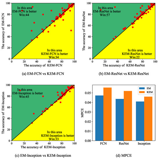
Figure 11.
Comparison between the EM-CNN and KEM-CNN. (a) shows the comparison between EM-FCN and KEM-FCN, (b) shows the comparison between the EM-ResNet and KEM-ResNet, (c) shows the comparison between the EM-Inception and KEM-Inception, (d) shows the MPCE based on different backbone.
4.7. Computational Complexity
Compared to the conventional CNN, the extra parameters added in the EM-CNN come from the matching matrix M. The parameters learned in matrix M are proportional to the corresponding kernel size . Moreover, the number of matrices M is proportional to the number of kernels used in each layer and in layers L in the network. Hence, the overall parameter added in EM-CNN is as presented in Equation (13):
Compared to the parameter learned in the convolutional layers, as in Equation (14), the parameter added by the matching matrix M is at least times . Thus, the EM-CNN can overfit on the UCR archive. Therefore, the matching matrix M of the EM-CNN is fixed on each layer in the experiment. An experimental comparison between the EM-CNN and KEM-CNN is conducted in the next section to confirm the necessity of this:
5. Discussion
From the results shown in Table 2 and Figure 7, the performance of the EM-FCN, EM-ResNet, and EM-Inception are better than the FCN, ResNet, and Inception, respectively. Nevertheless, it should be noted that the EM-CNN is not better than the corresponding CNN in all the datasets and the base architecture is important to the performance. It is more helpful to combine the elastic matching mechanism with the CNN in the “motion” datasets such as “InlineSkate”, “UwaveGestureLibraryAll” because it is common for different people to perform the same movement for different durations. Moreover, as shown in Figure 9, the improvement from the elastic matching mechanism decreases as the number of layers increases. The reason is that temporal distortion is adjusted layer by layer. In the limiting case, if the temporal distortion disappears at some layer, it is expected that the EM-CNN degenerates to the CNN, and performance improvement also disappears.
Besides, EM-CNN is a static model because the matching matrix is fixed after the training is completed. Hence, it is not an optimal solution in theory. The probable solution is to train another auxiliary network to adjust the matching matrix according to the different inputs. Furthermore, despite the results shown in Figure 11, KEM-CNN still has a larger capacity to model the nonlinear relationship between the time series and convolutional kernels, in theory, it is meaningful to apply the KEM-CNN to the large-scale datasets.
6. Conclusions
In this paper, an elastic matching mechanism was proposed to learn the matching relationship between the time series and convolutional kernels. Experiments on the EM-FCN, EM-ResNet and EM-Inception show that this elastic matching mechanism is appropriate to assist CNN to model the nonliear alignment between the time series and convolutional kernels. As presented in the discussion, this elastic matching mechanism is also beneficial to CNN with a different number of layers and convolutional kernel sizes. Compared with the conventional CNN, the extra computational complexity from this elastic matching mechanism is small which ensures this elastic matching mechanism is flexible. In future work, we will consider combining the dynamic filter with the elastic matching mechanism to more complex applications such as multivariable time series classification and clustering.
Author Contributions
Methodology, K.O.; supervision, Y.H. and S.Z.; writing—original draft, K.O.; writing—review and editing, Y.H. and Y.Z. All authors have read and agreed to the published version of the manuscript.
Funding
This work was funded by the National Natural Science Foundation of China under Grant No. 61903373.
Institutional Review Board Statement
Not applicable.
Informed Consent Statement
Not applicable.
Data Availability Statement
The data used in this study is from the UCR archive which can be found here: http://www.timeseriesclassification.com/.
Conflicts of Interest
The authors declare no conflict of interest.
References
- Liu, C.L.; Hsaio, W.H.; Tu, Y.C. Time series classification with multivariate convolutional neural network. IEEE Trans. Ind. Electron. 2018, 66, 4788–4797. [Google Scholar] [CrossRef]
- Ordóñez, F.J.; Roggen, D. Deep convolutional and lstm recurrent neural networks for multimodal wearable activity recognition. Sensors 2016, 16, 115. [Google Scholar] [CrossRef] [Green Version]
- Graves, A.; Jaitly, N.; Mohamed, A. Hybrid speech recognition with deep bidirectional LSTM. In Proceedings of the 2013 IEEE Workshop on Automatic Speech Recognition and Understanding, Olomouc, Czech Republic, 8–13 December 2013; pp. 273–278. [Google Scholar]
- Übeyli, E.D. Wavelet/mixture of experts network structure for EEG signals classification. Expert Syst. Appl. 2008, 34, 1954–1962. [Google Scholar] [CrossRef]
- Lee, D.J.; Schoenberger, R.B.; Shiozawa, D.; Xu, X.; Zhan, P. Contour matching for a fish recognition and migration-monitoring system. In Two-and Three-Dimensional Vision Systems for Inspection, Control, and Metrology II; International Society for Optics and Photonics: Bellingham, WA, USA, 2004; Volume 5606, pp. 37–48. [Google Scholar]
- Fawaz, H.I.; Forestier, G.; Weber, J.; Idoumghar, L.; Muller, P.A. Deep learning for time series classification: A review. Data Min. Knowl. Discov. 2019, 33, 917–963. [Google Scholar] [CrossRef] [Green Version]
- Cai, X.; Xu, T.; Yi, J.; Huang, J.; Rajasekaran, S. DTWNet: A dynamic time warping network. In Advances in Neural Information Processing Systems; The MIT Press: Cambridge, MA, USA, 2019; pp. 11640–11650. [Google Scholar]
- Iwana, B.K.; Uchida, S. Time series classification using local distance-based features in multi-modal fusion networks. Pattern Recognit. 2020, 97, 107024. [Google Scholar] [CrossRef]
- Serra, J.; Arcos, J.L. An empirical evaluation of similarity measures for time series classification. Knowl.-Based Syst. 2014, 67, 305–314. [Google Scholar] [CrossRef] [Green Version]
- Zhao, J.; Itti, L. shapedtw: Shape dynamic time warping. Pattern Recognit. 2018, 74, 171–184. [Google Scholar] [CrossRef] [Green Version]
- Dau, H.A.; Bagnall, A.; Kamgar, K.; Yeh, C.C.M.; Zhu, Y.; Gharghabi, S.; Ratanamahatana, C.A.; Keogh, E. The UCR time series archive. IEEE/CAA J. Autom. Sin. 2019, 6, 1293–1305. [Google Scholar] [CrossRef]
- Ding, H.; Trajcevski, G.; Scheuermann, P.; Wang, X.; Keogh, E. Querying and mining of time series data: Experimental comparison of representations and distance measures. Proc. VLDB Endow. 2008, 1, 1542–1552. [Google Scholar] [CrossRef] [Green Version]
- Jeong, Y.S.; Jeong, M.K.; Omitaomu, O.A. Weighted dynamic time warping for time series classification. Pattern Recognit. 2011, 44, 2231–2240. [Google Scholar] [CrossRef]
- Sakoe, H.; Chiba, S. Dynamic programming algorithm optimization for spoken word recognition. IEEE Trans. Acoust. Speech Signal Process. 1978, 26, 43–49. [Google Scholar] [CrossRef] [Green Version]
- Itakura, F. Minimum prediction residual principle applied to speech recognition. IEEE Trans. Acoust. Speech Signal Process. 1975, 23, 67–72. [Google Scholar] [CrossRef]
- Górecki, T.; Łuczak, M. Using derivatives in time series classification. Data Min. Knowl. Discov. 2013, 26, 310–331. [Google Scholar] [CrossRef] [Green Version]
- Passalis, N.; Tefas, A.; Kanniainen, J.; Gabbouj, M.; Iosifidis, A. Deep Adaptive Input Normalization for Time Series Forecasting. IEEE Trans. Neural Netw. Learn. Syst. 2020, 31, 3760–3765. [Google Scholar] [CrossRef] [PubMed] [Green Version]
- Franceschi, J.Y.; Dieuleveut, A.; Jaggi, M. Unsupervised scalable representation learning for multivariate time series. In Advances in Neural Information Processing Systems; The MIT Press: Cambridge, MA, USA, 2019; pp. 4650–4661. [Google Scholar]
- Dennis, D.K.; Acar, D.; Mandikal, V.; Sadasivan, V.; Simhadri, H.; Saligrama, V.; Jain, P. Shallow RNNs: A method for accurate time-series classification on tiny devices. In Proceedings of the 33rd Conference on Neural Information Processing Systems (NeurIPS 2019), Vancouver, BC, Canada, 8–14 December 2019. [Google Scholar]
- Vincent, L.; Thome, N. Shape and time distortion loss for training deep time series forecasting models. In Advances in Neural Information Processing Systems; The MIT Press: Cambridge, MA, USA, 2019; pp. 4189–4201. [Google Scholar]
- Wang, J.; Wang, Z.; Li, J.; Wu, J. Multilevel wavelet decomposition network for interpretable time series analysis. In Proceedings of the 24th ACM SIGKDD International Conference on Knowledge Discovery & Data Mining, London, UK, 19–23 August 2018; pp. 2437–2446. [Google Scholar]
- Wang, Z.; Yan, W.; Oates, T. Time series classification from scratch with deep neural networks: A strong baseline. In Proceedings of the 2017 International Joint Conference on Neural Networks (IJCNN), Anchorage, AK, USA, 14–19 May 2017; pp. 1578–1585. [Google Scholar]
- Iwana, B.K.; Uchida, S. Dynamic Weight Alignment for Convolutional Neural Networks. arXiv 2017, arXiv:1712.06530. [Google Scholar]
- Fawaz, H.I.; Lucas, B.; Forestier, G.; Pelletier, C.; Schmidt, D.F.; Weber, J.; Webb, G.I.; Idoumghar, L.; Muller, P.A.; Petitjean, F. Inceptiontime: Finding alexnet for time series classification. Data Min. Knowl. Discov. 2020, 34, 1936–1962. [Google Scholar] [CrossRef]
- Gunasekar, S.; Woodworth, B.; Bhojanapalli, S.; Neyshabur, B.; Srebro, N. Implicit regularization in matrix factorization. In Proceedings of the 2018 Information Theory and Applications Workshop (ITA), San Diego, CA, USA, 11–16 February 2018; pp. 1–10. [Google Scholar]
- Liu, W.; Liu, Z.; Rehg, J.M.; Song, L. Neural similarity learning. In Advances in Neural Information Processing Systems; The MIT Press: Cambridge, MA, USA, 2019; pp. 5025–5036. [Google Scholar]
- Demšar, J. Statistical comparisons of classifiers over multiple data sets. J. Mach. Learn. Res. 2006, 7, 1–30. [Google Scholar]
- Bagnall, A.; Lines, J.; Bostrom, A.; Large, J.; Keogh, E. The great time series classification bake off: A review and experimental evaluation of recent algorithmic advances. Data Min. Knowl. Discov. 2017, 31, 606–660. [Google Scholar] [CrossRef] [Green Version]
- Kate, R.J. Using dynamic time warping distances as features for improved time series classification. Data Min. Knowl. Discov. 2016, 30, 283–312. [Google Scholar] [CrossRef]
- Vlachos, M.; Kollios, G.; Gunopulos, D. Discovering similar multidimensional trajectories. In Proceedings of the 18th International Conference on Data Engineering, San Jose, CA, USA, 26 February–1 March 2002; pp. 673–684. [Google Scholar]
- Chen, L.; Özsu, M.T.; Oria, V. Robust and fast similarity search for moving object trajectories. In Proceedings of the 2005 ACM SIGMOD International Conference on Management of Data, Baltimore, MD, USA, 14–16 June 2005; pp. 491–502. [Google Scholar]
- Marteau, P.F. Time warp edit distance with stiffness adjustment for time series matching. IEEE Trans. Pattern Anal. Mach. Intell. 2008, 31, 306–318. [Google Scholar] [CrossRef] [Green Version]
- Stefan, A.; Athitsos, V.; Das, G. The move-split-merge metric for time series. IEEE Trans. Knowl. Data Eng. 2012, 25, 1425–1438. [Google Scholar] [CrossRef] [Green Version]
- Lines, J.; Bagnall, A. Time series classification with ensembles of elastic distance measures. Data Min. Knowl. Discov. 2015, 29, 565–592. [Google Scholar] [CrossRef]
- Lines, J.; Taylor, S.; Bagnall, A. Time series classification with HIVE-COTE: The hierarchical vote collective of transformation-based ensembles. ACM Trans. Knowl. Discov. Data 2018, 12. [Google Scholar] [CrossRef] [Green Version]
- Tanisaro, P.; Heidemann, G. Time series classification using time warping invariant echo state networks. In Proceedings of the 2016 15th IEEE International Conference on Machine Learning and Applications (ICMLA), Anaheim, CA, USA, 18–20 December 2016; pp. 831–836. [Google Scholar]
Publisher’s Note: MDPI stays neutral with regard to jurisdictional claims in published maps and institutional affiliations. |
© 2021 by the authors. Licensee MDPI, Basel, Switzerland. This article is an open access article distributed under the terms and conditions of the Creative Commons Attribution (CC BY) license (https://creativecommons.org/licenses/by/4.0/).


