Article

Storing Set Families More Compactly with Top ZDDs

Graduate School of Information Technology and Science, The University of Tokyo, Tokyo 158-8557, Japan
*
Author to whom correspondence should be addressed.
Algorithms 2021, 14(6), 172; https://doi.org/10.3390/a14060172
Submission received: 15 March 2021 / Revised: 21 May 2021 / Accepted: 29 May 2021 / Published: 31 May 2021
(This article belongs to the Special Issue Algorithms and Data-Structures for Compressed Computation)

Abstract

:
Zero-suppressed Binary Decision Diagrams (ZDDs) are data structures for representing set families in a compressed form. With ZDDs, many valuable operations on set families can be done in time polynomial in ZDD size. In some cases, however, the size of ZDDs for representing large set families becomes too huge to store them in the main memory. This paper proposes top ZDD, a novel representation of ZDDs which uses less space than existing ones. The top ZDD is an extension of the top tree, which compresses trees, to compress directed acyclic graphs by sharing identical subgraphs. We prove that navigational operations on ZDDs can be done in time poly-logarithmic in ZDD size, and show that there exist set families for which the size of the top ZDD is exponentially smaller than that of the ZDD. We also show experimentally that our top ZDDs have smaller sizes than ZDDs for real data.

1. Introduction

Zero-suppressed Binary Decision Diagrams (ZDDs) [1] are data structures which are derived from Binary Decision Diagrams (BDDs) [2] and represent a family of sets (combinatorial sets) in a compressed form using Directed Acyclic Graphs (DAGs). ZDDs are data structures specialized for processing set families and it is known that sparse set families can be compressed well. ZDDs support binary operations between two families of sets in time polynomial in the size of the ZDDs. Because of these advantages, ZDDs are used for combinatorial optimization problems and enumeration problems. Although ZDDs were originally developed for VLSI logic design, it has been shown that they can also be used effectively for graph problems and combinatorial problems because set families are a fundamental concept that appears in various fields [3,4]. Various other application researches related to intelligent information processing have been published, for example, in the fields of data mining [5,6,7], probabilistic graphical models such as Bayesian network [8,9], and game theory [10].
Though ZDDs can store set families compactly, their size may grow for some set families, and we need further compression. DenseZDDs [11] are data structures for storing ZDDs in a compressed form and supporting operations on the compressed representation. DenseZDDs represent a ZDD by a spanning tree of the DAG representing it, and an array of pointers between nodes on the spanning tree. Therefore its size is always linear to the original size, and to compress more, we need another representation.
Our basic idea for compression is as follows. In a ZDD, the identical sub-structures are shared and replaced by pointers. However identical sub-structures cannot be shared if they appear at different heights in ZDD. As a result, even if the DAG of a ZDD contains repetitive structures in the height direction, they cannot be shared.
For not DAGs but trees, there exists a data structure called top DAG compression [12], which can capture repetitive structures in the height direction. We extend it for DAGs and apply it to compress ZDDs which support the operations on compressed ZDDs.
This paper is an extended version of a conference paper published in SEA 2020 [13]. We rewrote the previous work so that readers not familiar with compression methods and operations on compressed data structure can understand our results easily. We added explanations of the DAG compression and how our algorithms work on compressed data with pseudo-codes. We also complement proof of space complexity.
The organization of the paper is as follows. In Section 2, we introduce our notation and data structures used throughout this paper. In Section 3, we introduce top trees and top DAGs. We show how to construct them and what operations they can perform. In Section 4, we propose our data structure, Top ZDD, and present the detailed components of Top ZDD, the theoretical analysis of the size, and the implementation method of the operations. In Section 5, we show the results of experiments for real and artificial data to evaluate construction time, search time and compactness of DenseZDDs. In Section 5, we show the experimental results on real and artificial data and compare Top ZDD, DenseZDD and standard ZDD to confirm the performance of the proposed method. In Section 6, we summarize the overall contents of this paper and discuss future work.

Our Contribution

We propose top ZDDs, which partition the edges of a ZDD into a spanning tree and other edges called complement edges, and store each of them in a compressed form. For the spanning tree, we use the top DAG compression, which represents a tree by a DAG with fewer nodes. For the complement edges, we store them in some nodes of the top DAG by sharing identical edges. We show that basic operations on ZDDs can be supported in O ( log 2 n ) time where n is the number of nodes of the ZDD. For further compression, we use succinct data structures for trees [14] and for bit vectors [15,16].
We show experimental results on the size of our top ZDDs and existing data structures, and query time on them. The results show that the top ZDDs use less space for most of the input data.

2. Preliminaries

Here we explain notations and basic data structures.
Let C = { 1 , , c } be the universal set. Any set in this paper is a subset of C. The empty set is denoted by . For a set S = { a 1 , , a s } C ( s 1 ) , its size is denoted by | S | = s . The size of the empty set is | | = 0 . A subset of the power set of C is called a set family. A set family is also called a family of sets, a set of sets, or a combinatorial set. If a set family F satisfies either S F k S , S { k } F or S F k C , S { k } F , F is said to be monotone. If the former is satisfied, F is monotone decreasing and the latter monotone increasing.

2.1. Zero-Suppressed Binary Decision Diagrams

Zero-suppressed Binary Decision Diagrams (ZDDs) [1] are data structures for manipulating finite set families. A ZDD is a directed acyclic graph (DAG) G = ( V , E ) with a root node satisfying the following properties. A ZDD has two types of nodes; branching nodes and terminal nodes. There are exactly two terminal nodes; ⊥ and ⊤. These terminal nodes have no outgoing edges. Each branching node v has an integer label ( v ) { 1 , , c } , and also has two outgoing edges 0-edge and 1-edge. The node pointed to by the 0-edge (1-edge) of v is denoted by v 0 = zero ( v ) ( v 1 = one ( v ) ). If for any branching node v it holds ( v ) < ( v 0 ) and ( v ) < ( v 1 ) , then the ZDD is said to be ordered. In this paper, we consider only ordered ZDDs. For convenience, we assume ( v ) = c + 1 for terminal nodes v. We divide the nodes of the ZDD into layers L 1 , , L c + 1 Note that if i j there are no edges from layer L i to layer L j . The number of nodes in ZDD G is denoted by | G | and called the size of the ZDD. On the other hand, the data size of a ZDD stands for the number of bits used in the data structure representing the ZDD.
In a ZDD, each node represents a set family. When a ZDD is single-rooted, the set family represented by the root is called the set family represented by the ZDD. The set family represented by a ZDD is defined as follows.
Definition 1
(The set family represented by a ZDD). Let v be a node of a ZDD and v 0 = zero ( v ) , v 1 = one ( v ) . Then the set family F v represented by v is defined as follows. ZDD G = ( V , E ) , rooted at node v V , represents a finite family of sets F v on C defined recursively as follows:
  • If v is a terminal node: if v = , F v = { } , if v = , F v = .
  • If v is a branching node: F v = { S { ( v ) } S F v 1 } F v 0 .
For the root node r of ZDD G, F r corresponds to the set family represented by the ZDD G. This set family is also denoted by F G .
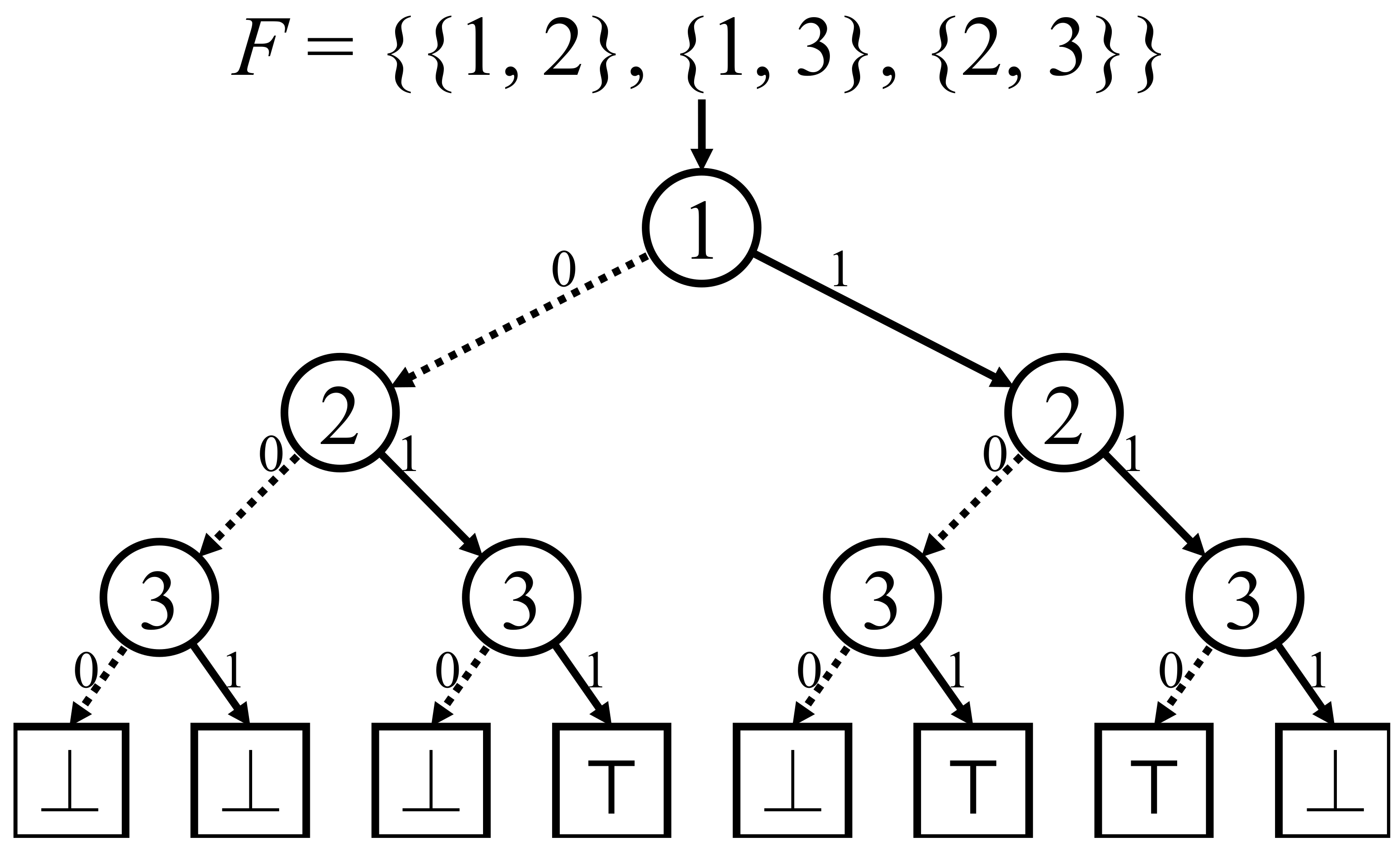
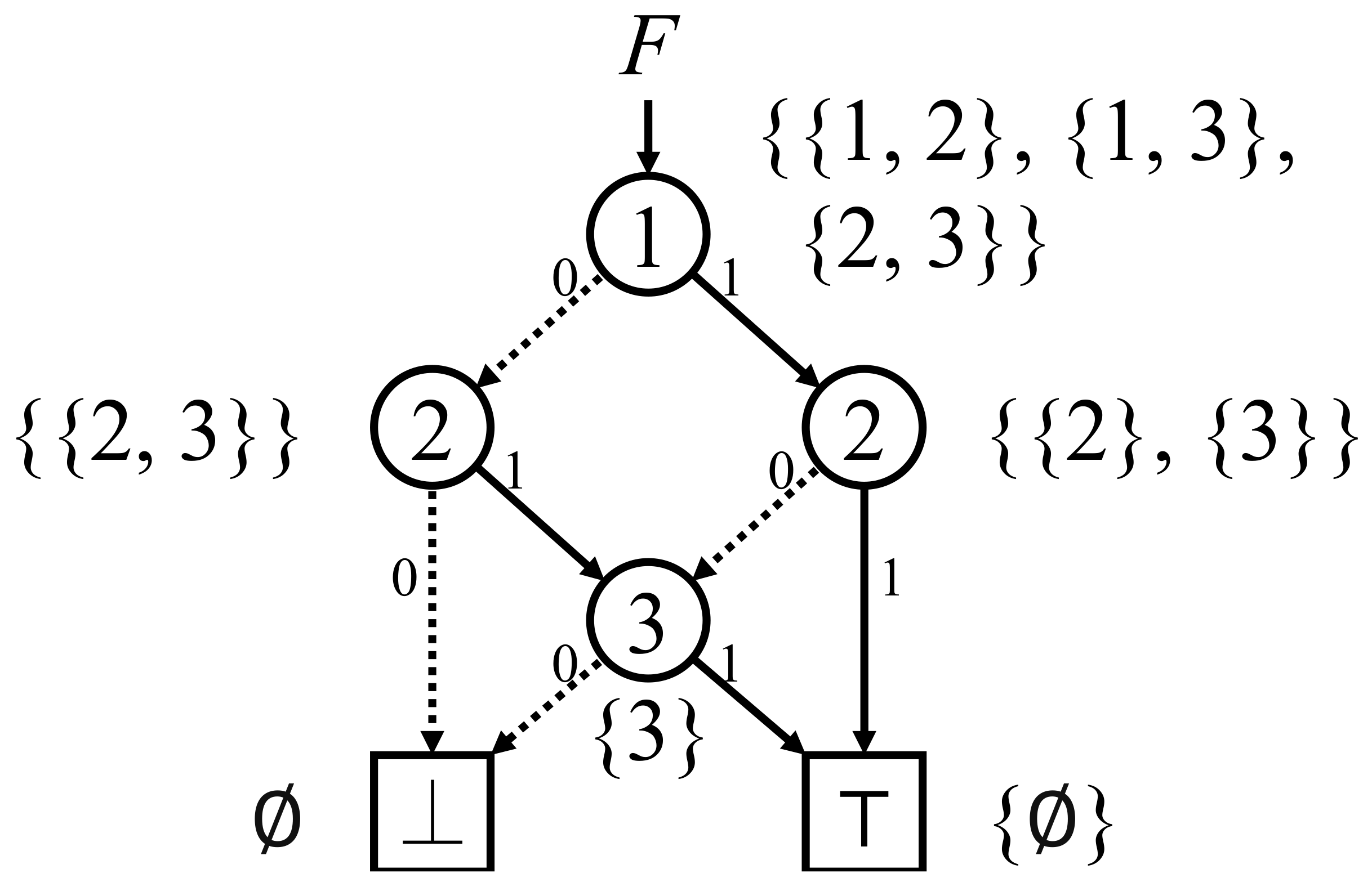
A family of sets can be represented by a binary tree as shown in Figure 1. Let F be a family of sets. For a set S, we traverse the 1-edge at the nodes whose labels are elements in S, and the 0-edge otherwise. Then we reach the ⊤ if S F , and the ⊥ otherwise. Any family of sets can be represented by a binary tree of height c. This is almost equivalent to the bitstring representation of length 2 n . This tree structure can be used for compression, however. A ZDD can be constructed by deleting redundant nodes from the binary tree and merging equivalent nodes. Every path from the root to the terminal ⊤ on ZDD G have a one-to-one correspondence to a set S = { a 1 , , a | S | } in the set family represented by G. Consider a traversal of nodes from the root towards terminals so that for each branching node v on the path, if ( v ) S we go to v 0 = zero ( v ) from v, and if ( v ) S we go to v 1 = one ( v ) from v. By repeating this process, if S F G we arrive at ⊤, and if S F G we arrive at ⊥ or find no branching node corresponding to some a i S during the process. An example is shown in Figure 2. ZDDs also support various set operations, which can be used to obtain new ZDDs from multiple ZDDs, as shown in Figure 3.

2.2. Succinct Data Structures

Succinct data structures are data structures whose size match the information-theoretic lower bound. Formally, a data structure is succinct if any element of a finite set U with cardinality L is encoded in log 2 ( L ) + o ( log 2 ( L ) ) bits. In this paper, we use succinct data structures for bit-vectors and trees.

2.2.1. Bit Vectors

Bit vectors are the most basic succinct data structures. A length-n sequence B { 0 , 1 } n of 0’s and 1’s is called a bit vector. On this bit vector we consider the following operations:
  • a c c e s s ( B , i ) ( 1 i n ): returns B [ i ] { 0 , 1 } , the i-th entry of B.
  • r a n k c ( B , i ) ( 1 i n , c = 0 , 1 ): returns the number of c in the first i bits of B.
  • s e l e c t c ( B , j ) ( 1 j n , c = 0 , 1 ): returns the position of the j-th occurrence of c in B.
The following result is known.
Theorem 1.
([15]) For a bit vector of length n, using a n + O ( n log log n / log n ) -bit data structure constructed in O ( n ) time, a c c e s s ( B , i ) , r a n k c ( B , i ) , s e l e c t c ( B , j ) are computed in constant time on the word-RAM with word length Ω ( log n ) .
Consider a bit vector of length n with m 1’s. For sparse bit vectors, namely, that consisting of a binary sequence with only m = o ( n / log n ) 1’s, we can obtain a more space-efficient data structure.
Theorem 2.
([16]) For a bit vector B of length n = 2 w with m ones, s e l e c t 1 ( B , i ) is computed in constant time using a 2 m + O ( m log log m / log m ) -bit data structure.
Note that on this data structure, r a n k 0 , r a n k 1 , s e l e c t 0 takes O ( log m ) time.

2.2.2. Trees

Consider a rooted ordered tree with n nodes. The information-theoretic lower bound on the size of such trees is 2 n Θ ( log n ) bits. When we traverse a tree by depth-first search and number each node in the order of the first visit, the number is called the preorder id of the node. When nodes are given ids, we may refer to each node as its number. We want to support the following operations:
  • p a r e n t ( x ) : returns the parent of node x.
  • f i r s t c h i l d ( x ) , l a s t c h i l d ( x ) : returns the first/last child of node x.
  • n e x t s i b l i n g ( x ) , p r e v s i b l i n g ( x ) : returns the next/previous sibling of node x.
  • i s l e a f ( x ) : returns if node x is a leaf or not.
  • p r e o r d e r _ r a n k ( x ) : returns the preorder id of node x.
  • p r e o r d e r _ s e l e c t ( i ) : returns the node with preorder id i.
  • l e a f _ r a n k ( x ) : returns the number of leaves whose preorder ids are smaller than that of node x.
  • l e a f _ s e l e c t ( i ) : returns the i-th leaf in preorder.
  • d e p t h ( x ) : returns the depth of node x, that is, the distance from the root to x.
  • s u b t r e e s i z e ( x ) : returns the number of nodes in the subtree rooted at node x.
  • l c a ( x , y ) : returns the lowest common ancestor (LCA) between nodes x and y.
Theorem 3.
([14]) On the word-RAM with word length Ω ( log n ) , the above operations are done in constant time using a 2 n + o ( n ) -bits data structure.
We call this the balanced parenthesis (BP) representation in this paper.

2.3. DenseZDD

A DenseZDD [11] is a static representation of a ZDD with attributed edges [17] by using some succinct data structures. In comparison to the standard ZDD, a DenseZDD provides a much faster membership operation and less memory usage for most cases. When we construct a DenseZDD from a given ZDD, dummy nodes are inserted so that ( v 0 ) = ( v ) + 1 holds for each branching node v for fast traversal. A Spanning Tree consisting of all inverted 0-edges is represented by a simple BP. Notice that, each node always has one 0-edge, and ZDDs have no cycles and the terminal node is only ⊥ if we employ the attributed edge technique. Therefore, if you traverse only the 0-edges from any branching node, you will always end up at the ⊥. The inverted 0-edges thus form a spanning tree rooted at the ⊥. The DenseZDD is a combination of this BP and other succinct data structures that represent the remaining information of the given ZDD. Its size is much smaller than the standard ZDD size and it can execute fast membership operations. A DenseZDD represents 0-edges and 1-edges respectively in a different way. For 0-edges, the spanning tree of a ZDD formed by the 0-edges is stored. We give preorder id for each node by a depth-first traversal of the spanning tree. Some dummy nodes are added such that ( v 0 ) = ( v ) + 1 holds for each node v. Spanning tree and dummy node information are represented by BP and Fully Indexable Dictionary (FID), respectively. For 1-edges, an array stores all the preorder ids of 1-children together.

3. Top Tree and Top DAG

We explain DAG compression [18,19,20] and top DAG compression [12] to compress labeled rooted trees.

3.1. DAG Compression

DAG compression is a scheme to represent a labelled rooted tree by a smaller DAG by sharing identical subtrees appearing repeatedly. See Figure 4 for an example.
When we repeat sharing common sub-structures until the sub-structure rooted at each node u becomes unique, the resulting structure is called the minimal DAG. The minimal DAG is unique and it can be obtained in O ( n ) time for a tree with n nodes [19]. We call representing a tree by the minimal DAG as DAG compression. After DAG compression, the number of nodes may be exponentially smaller than the original tree. On the other hand, in the worst case, the number of nodes never decreases. This is because DAG compression can share only identical subtrees. Here a subtree means the tree consisting of all the descendants of a node. For example, a path in which all nodes have the same label can be represented by just storing the length of the path and the label, DAG compression cannot capture this repeated structure and cannot compress the path.

3.2. Top DAG Compression

Top DAG compression is a compression scheme for labelled rooted trees by converting the input tree into top tree [21] and then compress it by DAG compression [18,19,20]. Top DAG compression can compress repeated sub-structures (not only subtrees). DAG compression can share identical subtrees, but it cannot share similar structures at different heights. This is made possible by top DAG compression. For example, a path of length n with identical labels cannot be compressed at all by DAG compression but can be represented by a top DAG with O ( log n ) nodes. Also, for a tree with n nodes, top DAG supports the following operations in O ( log n ) time: accessing a node label, computing the subtree size, and tree navigational operations such as first child and parent. Here we explain the top tree and its greedy construction algorithm. We also explain operations on top DAGs.

3.2.1. Top Tree

The top tree [21] for a labelled rooted tree T is a binary tree T representing the merging process of clusters of T defined as follows. A top tree is a meta-binary tree for managing tree structure, and its purpose is to transform a given tree into a somewhat balanced binary tree. We assume that all edges in the tree are directed from the root towards leaves, and an edge ( u , v ) denotes the edge from node u to node v. Clusters are subsets of T with the following properties.
  • A cluster is a subset F of the nodes of the original tree T such that nodes in F are connected in T.
  • F forms a tree and we regard the node in F closest to the root of T as the root of the tree. We call the root of F as the top boundary node.
  • F contains at most one node having directed edges to outside of F. If there is such a node, it is called the bottom boundary node.
A boundary node is either a top boundary node or a bottom boundary node.
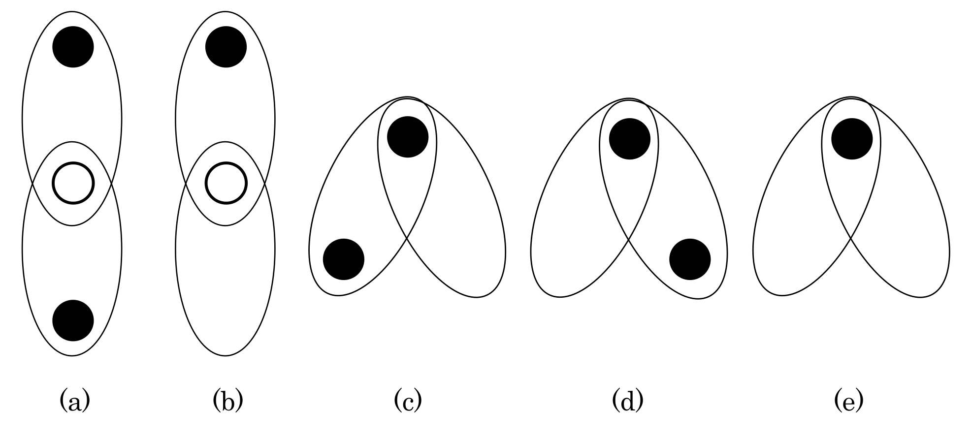
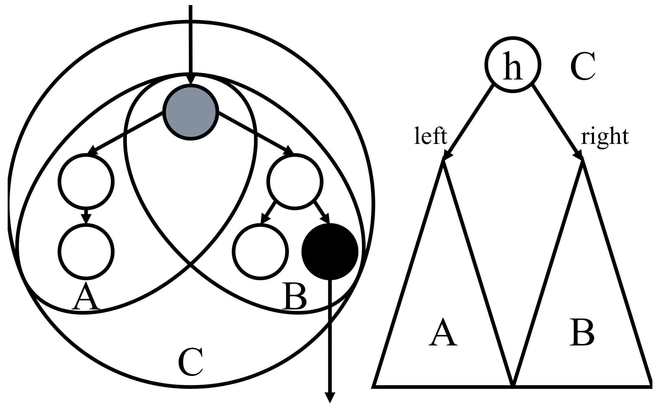
By merging two adjacent clusters, we obtain a new cluster, where merge means to take the union of node sets of two clusters and make it the node-set of the new cluster. There are five types of merges, as shown in Figure 5. In the figure, ellipses are clusters before merge, black circles are boundary nodes of new clusters, and white circles are not boundary nodes in new clusters.
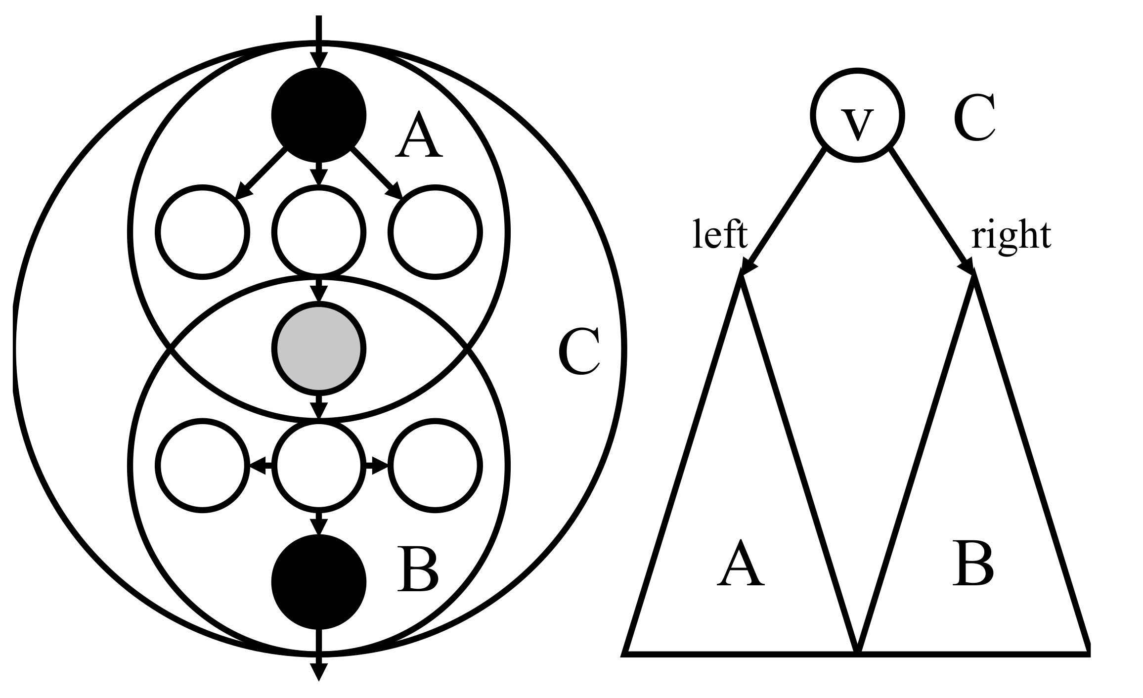
Examples of merge are shown in Figure 6 and Figure 7.
The top tree of the tree T is a binary tree T satisfying the following conditions. Note that we use terms nodes and edges for the original tree T, and vertices and arcs for the top tree T .
  • Each leaf of the top tree corresponds to a cluster with the endpoints of an edge of T.
  • Each internal vertex of the top tree corresponds to the cluster made by merging the clusters of its two children. This merge is one of the five types in Figure 5.
  • The cluster of the root of the top tree is T itself.
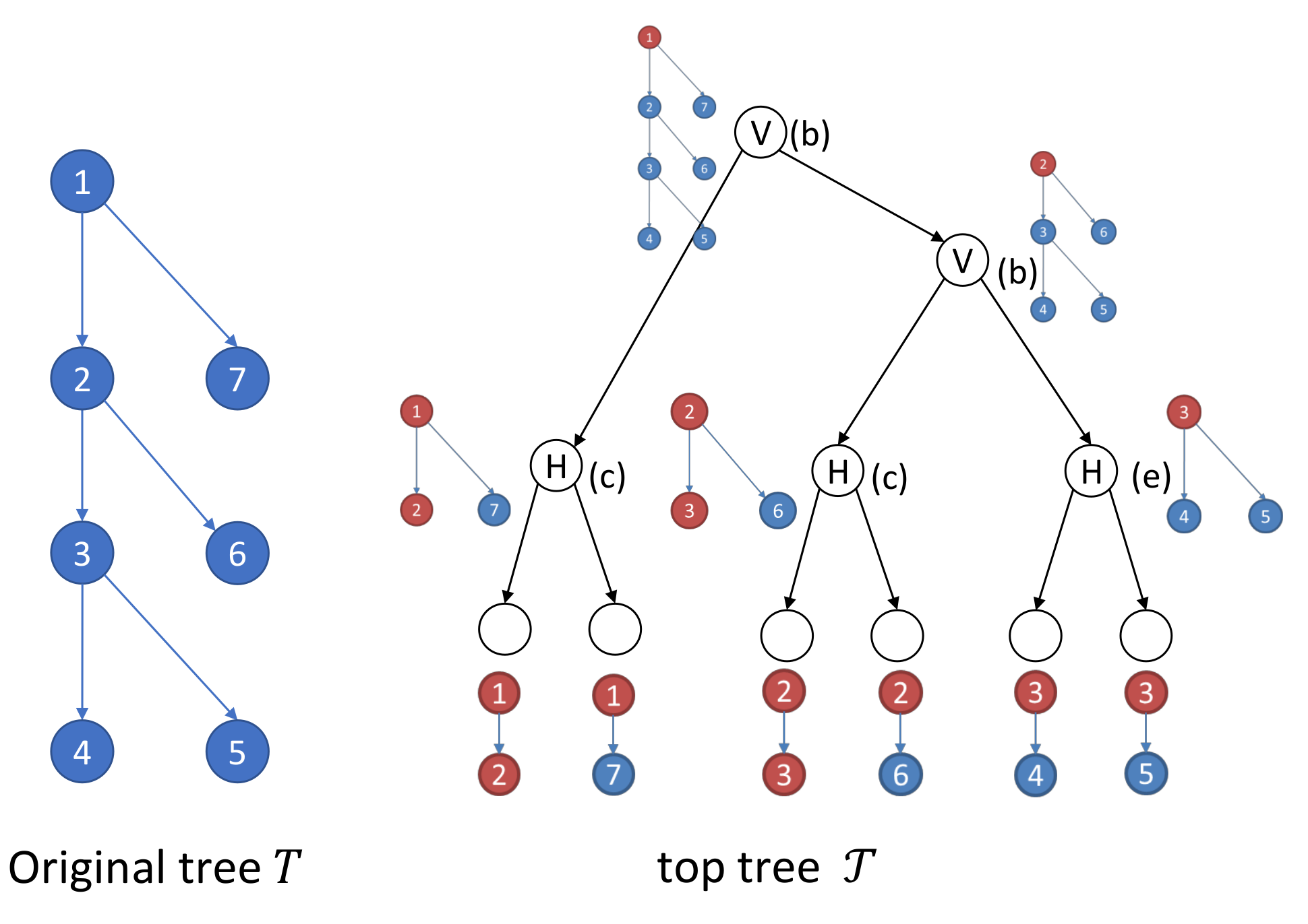
Figure 8 is an example of the top tree T for an unlabeled tree T.
V and H in vertices of the top tree represent vertical and horizontal merges, respectively. Letters on the right of vertices show the type of merges in Figure 5. Clusters corresponding to vertices of the top tree are also shown. Red nodes show boundary nodes of clusters.
We call the DAG obtained by DAG compression of the top tree T as top DAG T D , and the operation to compute the top DAG T D from tree T is called top DAG compression [12].
We define labels of vertices in the top tree to apply DAG compression as follows. For a leaf of the top tree, we define its label as the pair of labels of two endpoints of the corresponding edge in T. For an internal vertex of the top tree, its label must have information about cluster merge. It is enough to consider three types of merges, not five as in Figure 5. For vertical merges, it is not necessary to store the information that the merged cluster has a bottom boundary node or not. For horizontal merges, it is enough to store if the left cluster has a bottom boundary node or not. From this observation, we define labels of internal vertices as follows.
  • For vertices corresponding to vertical merge: we set their labels as V.
  • For vertices corresponding to horizontal merge: we set their labels as H L if the left child cluster has the bottom boundary node, or H R if the right child cluster has the bottom boundary node. If both children do not have bottom boundary nodes, the label can be arbitrary.
Top trees created by a greedy algorithm satisfy the following.
Theorem 4.
([12]) Let n be the number of nodes of a tree T. Then the height of top tree T created by a greedy algorithm is O ( log n ) .

3.2.2. Operations on Top DAGs

Consider to support operations on a tree T which is represented by top DAG T D . From now on, a node x in T stands for the node with preorder id x in T. By storing additional information to each vertex of the top DAG, the following tree operations can be supported [12].
  • A c c e s s ( x ) : returns the label of x.
  • D e c o m p r e s s ( x ) : returns the subtree T ( x ) of T rooted at x.
  • P a r e n t ( x ) : returns the preorder id of the parent of x.
  • D e p t h ( x ) : returns the depth, i.e., the distance to the root, of x.
  • H e i g h t ( x ) : returns the height, i.e., the distance to the farthest leaf, of x.
  • S i z e ( x ) : returns the subtree size rooted at x.
  • F i r s t c h i l d ( x ) : returns the preorder id of the first child of x, or reports x is a leaf.
  • N e x t S i b l i n g ( x ) : returns the preorder id of the next sibling of x, or reports it does not exist.
  • L e v e l A n c e s t o r ( x , i ) : returns the preorder id of the ancestor of x with distance i from x.
  • L C A ( x , y ) : returns the preorder id of the lowest common ancestor between x and y.
For a tree with n nodes, all operations except D e c o m p r e s s ( · ) are done in O ( log n ) time, and D e c o m p r e s s ( · ) is done in O ( log n + | T ( x ) | ) time.
We explain the algorithm for A c c e s s ( x ) based on a recursive function s u b ( u , k ) for a vertex u of the top DAG and an integer k. The function s u b ( u , k ) returns the label of the node with local preorder id k inside the cluster corresponding to vertex u of the top DAG. Note that A c c e s s ( x ) can be achieved by doing s u b ( r , x ) because the cluster corresponding to r is the whole tree. The function s u b ( u , k ) is computed recursively as follows. If u has no outgoing edges, u is a leaf of the top DAG. Thus, u corresponds to a cluster consisting of a single edge. In this case k is either 0 or 1. For such a cluster, only the label of the two endpoints of the edge is stored. Let s and t be the label of the starting point and ending point, respectively. If k = 0 , it returns s u b ( u , k ) = s ; if k = 1 , it returns s u b ( u , k ) = t .
If u is a vertex corresponding to horizontal merge, let v and w be the left and the right child of u, respectively, let c l ( u ) , c l ( v ) , c l ( w ) be the corresponding cluster of u , v , w , respectively, and let C ( u ) , C ( v ) , C ( w ) be their sizes. If we traverse nodes of c l ( u ) in preorder, the first one is the node shared by c l ( v ) and c l ( w ) , then all the nodes of c l ( v ) appear and finally nodes of c l ( w ) are traversed. Therefore s u b ( u , k ) is computed as follows.
  • If k = 1 : the corresponding node for s u b ( u , k ) is contained in both c l ( v ) and c l ( w ) , and it holds s u b ( u , k ) = s u b ( v , 1 ) = s u b ( w , 1 ) .
  • If 2 k C ( v ) : the corresponding node for s u b ( u , k ) is in c l ( v ) , and it holds s u b ( u , k ) = s u b ( v , k ) .
  • If C ( v ) + 1 k C ( v ) + C ( w ) 1 : the corresponding node for s u b ( u , k ) is in c l ( w ) , and it holds s u b ( u , k ) = s u b ( w , k C ( v ) + 1 ) .
This function can be computed if the cluster size C ( · ) is known for each vertex of the top DAG.
Finally, if u is a vertex corresponding to vertical merge, define v, w, c l ( u ) , c l ( v ) , c l ( w ) , C ( u ) , C ( v ) , C ( w ) similarly to the horizontal merge case. We need another value D ( v ) , which is the preorder id of the bottom boundary of c l ( v ) . If we traverse nodes of c l ( u ) in preorder, we first visit nodes of c l ( v ) with local preorder id up to D ( v ) , then visit all nodes of c l ( w ) , then finally visit nodes of c l ( v ) with local preorder id from D ( v ) + 1 . Therefore s u b ( u , k ) is computed as follows.
  • If 1 k D ( v ) 1 : the corresponding node for s u b ( u , k ) is in c l ( v ) , and it holds s u b ( u , k ) = s u b ( v , k ) .
  • If k = D ( v ) : the corresponding node for s u b ( u , k ) is the bottom boundary node of c l ( v ) , which is also the top boundary node of c l ( w ) , and it holds s u b ( u , k ) = s u b ( v , k ) = s u b ( w , 1 ) .
  • If D ( v ) + 1 k D ( v ) + C ( w ) : the corresponding node for s u b ( u , k ) is in c l ( w ) , and it holds s u b ( u , k ) = s u b ( w , k D ( v ) 1 ) .
  • If D ( v ) + C ( w ) + 1 k C ( v ) + C ( w ) 1 : the corresponding node for s u b ( u , k ) is in c l ( v ) , and it holds s u b ( u , k ) = s u b ( v , k C ( w ) 1 ) .
This function can be computed recursively if C ( · ) and D ( · ) are known. Algorithm 1 shows a pseudo code.
Algorithm 1  A c c e s s ( x ) : computes the label of a node whose preorder id in the tree representing the top DAG is x.
  • Input: Preorder x
  • Output: The label of node x
    1:
    r the root of top DAG
    2:
    return SUB ( r , x )
    3:
    procedure SUB( u , k )
    4:
        if vertex u corresponds to a cluster with a single edge e then
    5:
            if  k = 1  then
    6:
               return (the label s of the starting point of e)
    7:
            else
    8:
               return (the label s of the ending point of e)
    9:
        else
    10:
             v ( the left child of   u )
    11:
             w ( the right child of   u )
    12:
             C ( v ) ( the size of the cluster of   v )
    13:
             C ( w ) ( the size of the cluster of   w )
    14:
            if vertex u is horizontal merge then
    15:
               if  1 k C ( v )  then
    16:
                   return  SUB ( v , k )
    17:
               else
    18:
                   return  SUB ( w , k C ( v ) 1 )
    19:
            else
    20:
                D ( v ) ( the preorder id of the bottom boundary node of the cluster of   v )
    21:
               if  1 k D ( v )  then
    22:
                   return  SUB ( v , k )
    23:
               else if  D ( v ) + 1 k D ( v ) + C ( w )  then
    24:
                   return  SUB ( w , k D ( v ) 1 )
    25:
               else
    26:
                   return  SUB ( v , k C ( w ) 1 )

4. Top ZDD

We explain our top ZDD, which is a representation of ZDD by top DAG compression. Though it is easy to apply our compression scheme for general rooted DAGs, we consider the only compression of ZDDs.
A ZDD G = ( V , E ) is a directed acyclic graph in which branching nodes have labels ( · ) and edges have labels 0 or 1. We can regard it as a graph with only edges being labelled. For each edge ( u , v ) of ZDD G, we define its label as a pair (edge label 0/1, ( v ) ( u ) ) if v is a branching node, or a pair (edge label 0/1, ⊥/⊤) if v is a terminal node. Note that in the second case, we are not taking the difference of labels. We only care whether the terminal is ⊤ or ⊥. In practice, we can use c + 1 instead of ⊥, and c + 2 instead of ⊤ for the second element of the second case. It is enough to distinguish the above two cases because ( v ) ( u ) is always less than c for any u , v . Below we assume ZDDs have labels for only edges, and 0-edge comes before 1-edge for each node.
Next, we consider top trees for edge-labelled trees. The difference from node-labelled trees is only how to store the information for single edge clusters. In Section 3.2.1, we stored labels for both endpoints of edges. We change this for storing only edge labels.
The top ZDD is constructed from a ZDD G = ( V , E ) as follows.
  • We perform a depth-first traversal from the root of G and obtain a spanning tree T of all branching nodes. During the process, we do not distinguish 0-edges and 1-edges, and terminal nodes are not included in the tree. Nodes of the tree are identified with their preorder ids in T. If we say node u, it means the node in T with preorder id u. We call edges of G not included in T as complement edges.
  • We convert the spanning tree T to a top tree T by the greedy algorithm.
  • For each complement edge ( u , v ) , we store its information in a node of T as follows. If v is a terminal, let a be the vertex of the top tree corresponding to the cluster of a single edge between u and its parent in T. Note that a is uniquely determined. Then we store a triple ( ( u , v ) , edge label 0/1, ⊥/⊤) in a. If v is a branching node, we store the information of the complement edge to a vertex of T corresponding to a cluster containing both u and v. The information to store is a triple ( ( u , v ) , edge label 0/1, ( u ) ( v ) ). Each vertex stores such information as follows. Let a , b be the vertices of the top tree corresponding to the clusters of single edges towards u , v in T, respectively. Then we store the triple in the lowest common ancestor lca ( a , b ) in T. Here the information ( u , v ) represents local preorder ids inside the cluster corresponding to lca ( a , b ) . Note that lca ( a , b ) may not be the minimal cluster including both u and v.
  • We create a top DAG T D by DAG compression by sharing identical clusters. To determine the identity of two clusters, we compare them together with the information of complement edges in the clusters stored in step 3. Complement edges that do not appear in multiple clusters are moved to the root of T.
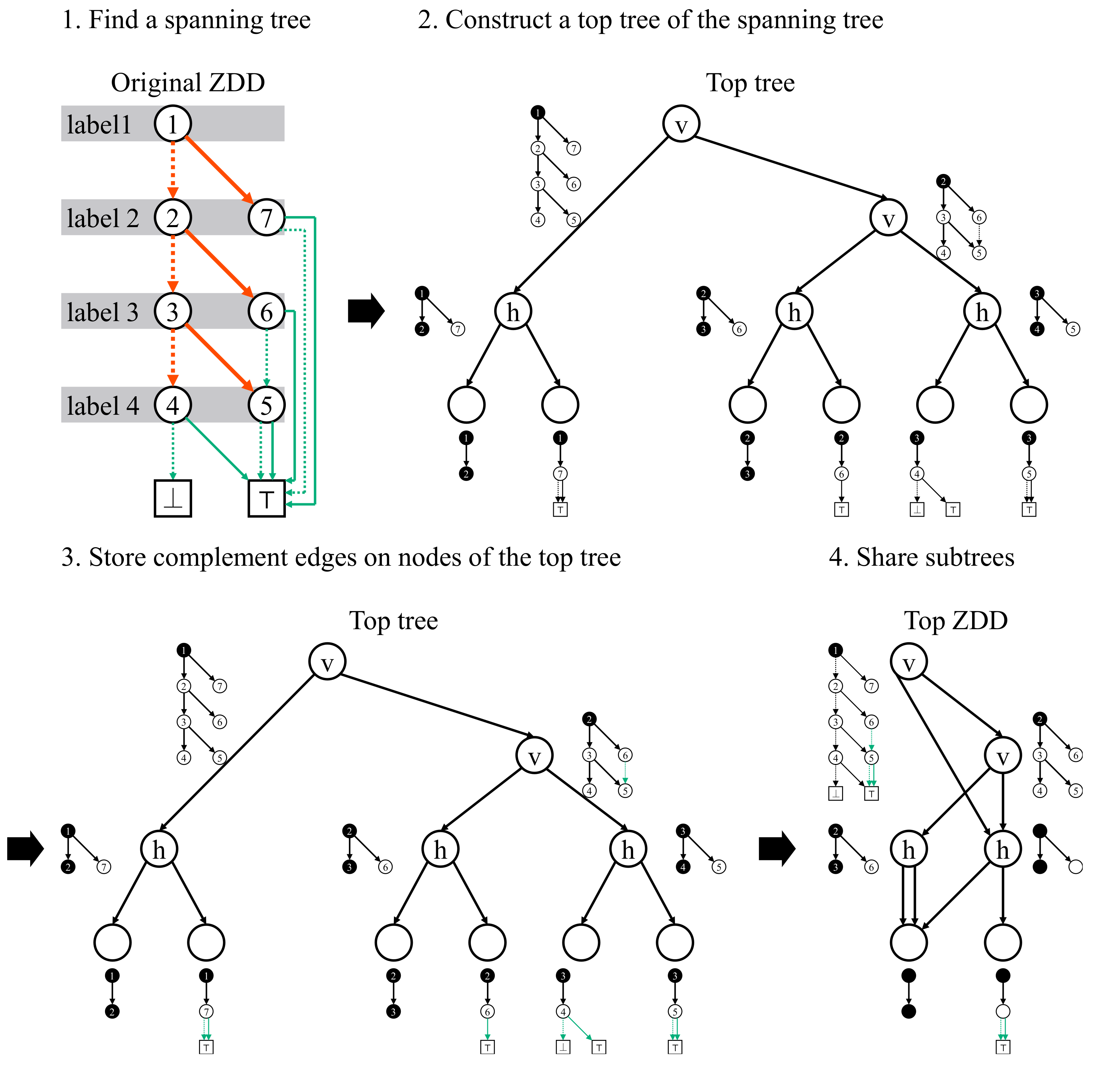
Figure 9 shows an example of how our algorithm works. In this figure, we show the clusters corresponding to each node. But, they are not stored explicitly.
It is crucial to choose an appropriate data structure to store each information to achieve smaller space consumption. For example, in Section 3.2.2, we explained that each vertex of the top DAG stores the cluster size etc., this is redundant and space can be reduced. Next, we explain our space-efficient data structure which is enough to support efficient queries in detail.

4.1. Details of the Data Structure

We need the following information to recover the original ZDD from a top ZDD.
  • Information about the structure of top DAG T D .
  • Information about each vertex of T D . There are three types of vertices: vertices corresponding to a leaf of the top tree, vertices representing vertical merge, and vertices representing horizontal merge. For each type, we store different information.
  • Information about complement edges.
We show space-efficient data structures for storing this information. The data structure to be used is chosen depending on the ratio of 1’s. If the ratio of 1’s is less than 1 4 , then we use the SparseArray [22] to compress a bit vector. Or if the ratio of 1’s is between 1 4 and 3 4 , then we use the succinct bit vector with constant time rank/select support [15].
And, we use the SparseArray for the bit vector whose 0/1 are flipped if the ratio of 0’s is less than 1 4 . To store an array of non-negative integers, we use log 2 m bits for each entry where m is the maximum value in the array. Let n denote the number of branching nodes of a ZDD. We use n + 1 , n + 2 to represent terminals , , respectively.

4.1.1. The Data Structure for the Structure of Top DAG T D

We store top DAG T D after converting it to a tree. We make tree T by adding dummy vertices to T D . For each vertex x of T D whose in-degree is two or more, we do the following.
  • Let a 1 , , a t be the vertices of T D from which there are edges towards x. Note that there may exist identical vertices among them corresponding to different edges. We create t 1 dummy vertices d 1 , , d t 1 .
  • For each 1 i t 1 , remove edge ( a i , x ) and add edge ( a i , d i ) .
  • For each dummy vertex d i , we store information about a pointer to x. In our implementation, we store the preorder id of x in T from which the dummy vertices are removed.
Then we can represent the structure of the top DAG by the tree T and the pointers from the dummy vertices.
Next, we explain how to store T and the information about the dummy vertices. The structure of T is represented by the BP sequence [14]. There are two types of leaves in T : those which exist in the original top DAG, and those for the dummy vertices. To distinguish them, we use a bit vector. Let m be the number of leaves in T . We create a bit vector B dummy of length m whose i-th bit corresponds to the i-th leaf of T in preorder. We set B dummy [ i ] = 1 if the i-th leaf is a dummy vertex, and we set B dummy [ i ] = 0 otherwise.
We add additional information to dummy vertices to support efficient queries. We define an array clsize of length D where D is the number of dummy vertices. For the i-th dummy vertex in preorder, let s i be the vertex pointed to by the dummy vertex. We define clsize [ k ] = i = 1 k ( the number of vertices in the cluster represented by   s i ) . That is, clsize [ k ] stores the cumulative sum of cluster sizes up to k. This array is used to compute the cluster size for each vertex efficiently.

4.1.2. Information on Vertices

We explain how to store information on vertices of T except for dummy vertices. Each vertex corresponding to a leaf in the original top tree is a cluster for a single edge in the spanning tree, and it is a non-dummy leaf in T . We sort these vertices in preorder in T and store information on edges towards them in the following two arrays. One is an array label _ span to store differences of levels between endpoints of edges. Let u and v be the starting and the ending points of the single edge of the cluster corresponding to the i-th leaf, respectively. Then we set label _ span [ i ] = ( v ) ( u ) . The other is an array type _ span to store if an edge is 0-edge or 1-edge. We set type _ span [ i ] = 0 if the edge corresponding to the i-th vertex is a 0-edge, and type _ span [ i ] = 1 otherwise.
Each vertex of T corresponding to vertical merge or horizontal merge is an internal vertex. We sort internal vertices of T in their preorder. Then we make a bit vector B H so that B H [ i ] = 0 if the i-th vertex stands for vertical merge, and B H [ i ] = 1 if it stands for horizontal merge. For vertices corresponding to horizontal merge, we do not store additional information. For vertices corresponding to vertical merge, we use arrays preorder _ diff and label _ diff to store the differences of preorder ids and levels between the top and the bottom boundary nodes of the merged cluster. Let x i be the i-th vertex in preorder corresponding to vertical merge, c l i be the cluster corresponding to x i , t i be the top boundary node of c l i , and b i be the bottom boundary node of c l i . Note that t i and b i are nodes of the ZDD. Then we set preorder _ diff [ i ] = ( the local preorder id of   b i   inside cluster   c l i ) and label _ diff [ i ] = ( b i ) ( t i ) .

4.1.3. Information on Complement Edges

Complement edges are divided into two groups: those stored in the root of the top DAG and those stored in other vertices. We represent them differently.
First, we explain the data structure for storing complement edges in the root of the top DAG. Let E r o o t be the set of all complement edges stored in the root. We sort edges of E r o o t in the preorder of their starting point. Orders between edges with the same starting point are arbitrary.
For complement edges stored in the root, we store the preorder ids of their starting point using a bit vector B src _ root , the preorder ids of their ending point using an array dst _ root , and edge labels 0/1 using an array type _ root . The cluster corresponding to the root of the top DAG is the spanning tree of the ZDD. For each node v of the spanning tree, we represent the number of complement edges in E r o o t whose starting point is v, using a unary code. Unary code is a method of representing a natural number by the length of continuous 1’s. We concatenate and store them in preorder in the bit vector B src _ root . For edges in E r o o t sorted in preorder of the starting points, we store the preorder id of the ending point of the i-th edge in dst _ root [ i ] , and set type _ root [ i ] = 0 if the i-th edge is a 0-edge, and set type _ root [ i ] = 1 otherwise.
Next, we explain the data structure for storing complement edges in vertices other than the root. Let E i n be the set of those edges. We sort the edges as follows.
  • We assign each edge of E i n to a cluster such that it contains both its starting and ending points. Then, we divide E i n into several groups, each corresponding to a certain cluster. We sort these groups by the preorder id of the top tree vertex corresponding to the cluster.
  • Inside each cluster c l ( x ) , we sort the edges of E i n in preorder of starting points of the edges. For edges with the same starting point, their order is arbitrary.
We store the sorted edges of E i n using a bit vector B edge and three arrays src _ in , dst _ in , and type _ in . The bit vector B edge stores the numbers of complement edges in vertices of T by unary codes. The arrays src _ in , dst _ in , and type _ in are defined as: src _ in [ i ] = (the local preorder id of the starting point of the i-th edge inside the cluster), dst _ in [ i ] = ( the local preorder id of the ending point of the i-th edge inside the cluster), type _ in [ i ] = 0 if the i-th edge is a 0-edge, and type _ in [ i ] = 1 otherwise.
Table 1 summarizes the components of the top ZDD.

4.2. Size of Top ZDDs

The size of top ZDDs heavily depends on not only the number of vertices in the spanning tree after top DAG compression but also the number of complement edges for which we store some information. As a result, the size of top ZDDs becomes small if the number of nodes is reduced by top DAG compression and many common complement edges are shared.
In the best case, top ZDDs are exponentially smaller than ZDDs.
Theorem 5.
There exists a ZDD with n nodes to which the corresponding top ZDD has O ( log n ) vertices.
Proof. 
A ZDD storing a power set with n = 2 m elements satisfies the claim. Figure 10 shows this ZDD and top ZDD. A ZDD representing a power set have a linear chain-like shape because no matter how we traverse 0-edges or 1-edges, we will always end up at the ⊤ terminal. The spanning tree of the ZDD is a path consisting of 2 m many 0-edges. Its top tree has a leaf corresponding to a 0-edge of length 1, and internal vertices form a complete binary tree with height m. If we apply DAG compression to this top tree, we obtain the DAG of length m as shown in Figure 10. Sharing complement edges also works very well. The k-th vertex below representing vertical merge stores a 1-edge connecting a node with local preorder id 2 k 1 + 1 inside a cluster and a node with local preorder id 2 k 1 + 2 . The root of the top DAG stores 0-edge and 1-edge to the terminal ⊤. Because the height of the top DAG is O ( log n ) , the claim holds.  □

4.3. Operations on Top ZDDs

We give algorithms for supporting operations on the original ZDD using the top ZDD. We consider the following three basic operations. We identify each node x of the ZDD by its preorder id in the spanning tree T used to construct the top ZDD. An example of ZDD nodal numbering based on this rule is shown in the upper left corner of Figure 9.
  • ( x ) : returns the label of a branching node x.
  • z e r o ( x ) : returns the preorder id of the node pointed to by the 0-edge of x or returns ⊥ or ⊤ if the node is a terminal.
  • o n e ( x ) : returns the preorder id of the node pointed to by the 1-edge of x or returns ⊥ or ⊤ if the node is a terminal.
We show ( x ) is done in O ( log n ) time and other operations are done in O ( log 2 n ) time where n is the number of nodes of the ZDD. Below we denote the vertex of T stored in the top ZDD with preorder id x by “vertex x of T ”.
First we explain how to compute ( x ) in O ( log n ) time. We can compute ( x ) recursively using an algorithm similar to those on the top DAG. A difference is that in Section 3.2.2 we assumed that each vertex of the top DAG stores the cluster size, while in the top ZDD it is not stored to reduce the space requirement. Therefore we have to compute it using the information in Table 1.
To work the recursive computation, we need to compute the cluster size s i z e ( x ) represented by vertex x of T efficiently. We can compute s i z e ( x ) by the number of non-dummy leaves in the subtree of T rooted at x , and the sizes of the clusters corresponding to dummy leaves in the subtree rooted at x . If we merge two clusters of size a and b, the resulting cluster has size a + b 1 . Therefore if we merge k clusters whose total size is S, the resulting cluster after k 1 merges has size S k + 1 . These values can be computed from the BP sequence b p of T , the array clsize , and the bit vector B dummy . By using b p , we can compute the interval [ l , r ] of leaf ranks in the subtree rooted at x . Then, using B dummy , we can find the number c of non-dummy leaves and the interval [ l , r ] of non-dummy leaf ranks, in the subtree of x . Because clsize is the array for storing cumulative sums of cluster sizes for dummy leaves, the summation of sizes of clusters corresponding to l -th to r -th dummy leaves is obtained from clsize [ r ] clsize [ l 1 ] . Since the size of a cluster for a non-dummy leaf is always 2, the summation of cluster sizes for non-dummy leaves is also obtained. Algorithm 2 gives a pseudo-code for computing s i z e ( x ) . This can be done in constant time.
Algorithm 2  s i z e ( x ) : the size of the cluster corresponding to vertex x of T .
  • Input: Preorder x
  • Output: The size of the cluster for x
    1:
    l l e a f _ r a n k ( l e f t m o s t _ l e a f ( x ) )
    2:
    r l e a f _ r a n k ( r i g h t m o s t _ l e a f ( x ) )
    3:
    l r a n k 1 ( B dummy , l 1 ) + 1
    4:
    r r a n k 1 ( B dummy , r )
    5:
    k r l + 1
    6:
    c ( r l + 1 ) ( r l )
    7:
    if l = 0 then
    8:
        return  clsize [ r ] + 2 c k
    9:
    else
    10:
        return  clsize [ r ] clsize [ l 1 ] + 2 c k
Using the function s i z e ( x ) , we can compute a recursive function similar to Algorithm 1. Instead of D ( · ) in Algorithm 1, we use preorder _ diff . When we arrive at a dummy leaf, we use a value in dst _ dummy to move to the corresponding internal vertex of T and restart the recursive computation. Then for the vertex of the original ZDD whose preorder id in T is x, we can obtain the leaf of T corresponding to the cluster of a single edge containing x.
To compute ( x ) , we traverse the path from the root of T to the leaf corresponding to the cluster containing x. First we set s = 1 . During the traversal, if the current vertex is for vertical merge and the next vertex is its right child, that is, the next cluster is in the bottom, we add the label _ diff value of the top cluster to s. The index of label _ diff is computed from B H and b p . When we reach the leaf p of T , if x is its top boundary node, it holds ( x ) = s , otherwise, let k = l e a f _ r a n k ( p ) , then we obtain ( x ) = s + label _ span [ k r a n k 1 ( B dummy , k ) ] . Because each operation is done in constant time and the height of the top DAG is O ( log n ) , ( x ) is computed in O ( log n ) time.
Next, we show how to compute y = z e r o ( x ) . We can compute o n e ( x ) in a similar way. We do a recursive computation as operations on top DAG, a difference is how to process complement edges. There are two cases: if the 0-edge from x is in the spanning tree or not. If the 0-edge from x is in the spanning tree, the edge is stored in a cluster with a single edge ( x , y ) . The top boundary node of such a cluster is x. Therefore we search clusters whose top boundary node is x. If the 0-edge from x is not in the spanning tree, it is a complement edge and it is stored in some vertex on the path from a cluster C with a single edge whose bottom boundary node is x to the root. Therefore we search for C.
First, we recursively find a non-dummy leaf of T whose top boundary node is x. During this process, if there is a vertex whose top boundary is x and its cluster contains more than one edge and corresponds to horizontal merge, we move to the left child, because the 0-edge from x must exist in the left cluster. If we find a non-dummy leaf of T which corresponds to a cluster with a single edge and its top boundary node is x, its bottom boundary node is y = z e r o ( x ) . We climb up the tree until the root to compute the global preorder id of y. If there does not exist such a leaf, the 0-edge from x is not in the spanning tree. We find a cluster with a single edge whose bottom boundary node is x. From the definition of the top ZDD, the 0-edge from x is stored in some vertices visited during the traversal. Because complement edges stored in a cluster are sorted in local preorder ids inside the cluster of starting points, we can check if there exists a 0-edge whose starting point is x in O ( log n ) time. If it exists, we obtain the local preorder id of y inside the cluster. By going back to the root, we obtain the global preorder id of y. Note that complement edges for all clusters are stored in one array, and therefore we need to obtain the interval of indices of the array corresponding to a cluster. This can be done using B edge . In the worst case, we perform a binary search in each cluster on the search path. Therefore the time complexity of z e r o ( x ) is O ( log 2 n ) .

5. Experimental Comparison

We compare our top ZDD with existing data structures. We implemented top ZDD with C++ and measured the required space for storing the data structure. For comparison, we used the following three data structures.
  • top ZDD (proposed): we measured the space for storing the data structures in Table 1.
  • DenseZDD [11]: data structures for representing ZDDs using succinct data structures. Two data structures are proposed; one support constant time queries and the other has O ( log n ) time complexity. We used the latter that uses less space.
  • a standard ZDD: a data structure which naively represents ZDDs. We store for each node its label and two pointers corresponding to a 0-edge and a 1-edge. Space is 2 n log n + n log c bits where n is the number of nodes of a ZDD and c is the size of the universe of a set family.
We constructed ZDDs of the following set families.
  • The power set of a set { 1 , , A } with A elements.
  • For the set { 1 , , A } with A elements, the family of all the set S satisfying
    ( The maximum value of   S ) ( The minimum value of   S ) B .
  • For the set { 1 , , A } with A elements, the family of all the sets with cardinality at most B.
  • Knapsack set families with random weights. That is, for i-th element in a set ( 1 i A ), we define its weight w i as a uniformly random integer in [ 1 , W ] , then sort the elements in decreasing order of weights, and construct a set family consisting of all sets with weight at most C. Because of the randomness of the input, we ran the experiment 1024 times for each setting and calculate the t-value and p-value between top ZDD and DenseZDD.
  • The family of edge sets which are a matching of a given graph. As for graphs, we used the 8 × 8 grid graph, the complete graph with 12 vertices K 12 , and a real communication network “Interoute”.
  • Set families of frequent itemsets.
  • Families of edge sets which are paths from the bottom left vertex to the top-right vertex in n × n grid graph, for n = 6 , 7 , 8 , 9 .
  • Families of solutions of the n-queen problem (The n-queen problem is to find an arrangement of n queens on the n × n chessboard such that no two queens threaten each other. Here, all possible arrangements are stored in a ZDD), for n = 11 , 12 , 13 .
We used several values for the parameters A , B , C , W . The results are shown in Table 2, Table 3, Table 4, Table 5, Table 6, Table 7, Table 8 and Table 9. The unit of size is a byte.
We found that for all data sets, the top ZDD uses less space than the theoretical size of the standard ZDD. We also confirmed that the data sets in Table 2, Table 3 and Table 4 can be compressed very well by top ZDDs. Table 5 shows the results on the sets of solutions of knapsack problems. Top ZDD uses less space than DenseZDD in all cases, and in some cases, the memory usage of top ZDD is almost half that of DenseZDD. Table 6 and Table 7 show the results for families of matching in a graph and frequent itemsets, respectively. There are a few cases where the DenseZDD uses less space than the top ZDD.
The results above are for monotone set families, that is, any subset of the set of the family also exists in the family. Table 8 and Table 9 show results on non-monotone set families. For the set of edges on the path from the bottom left corner to the top right corner of an n × n grid graph, the top ZDD uses less space than the DenseZDD, and for n = 9 , the top ZDD uses about 1 / 3 the memory of DenseZDD. On the other hand, for the sets of all the solutions of the n-queen problem, the top ZDD uses about 10% more space than the DenseZDD. From these experiments, we confirmed that top ZDD uses less space than DenseZDD for many set families.
Next, we show the construction time and edge traversal time of the top ZDD and the DenseZDD in Table 10, Table 11, Table 12, Table 13, Table 14, Table 15, Table 16 and Table 17. For edge traversal time, we traversed from the root of a ZDD towards terminals by randomly choosing 0- or 1-edge 65,536 times, and took the average. When we arrived at a terminal, we restarted from the root.
In almost all cases, the Top ZDD construction took 1.5 to 2.5 times longer than the DenseZDD construction. The first data in Table 11 and the third data in Table 13 took particularly a long time, suggesting that DenseZDD is faster for families of sets where the size of the included sets is small compared to the total number of variables. The same reason is expected for the overall slowness of Top ZDD for n-queen problems. The second data of Table 15 is the only case that Top ZDD is constructed faster than DenseZDD. This is probably because this data is hardly compressed and DenseZDD is worse than the theoretical size of ordinary ZDD. In terms of traversal time, Top ZDD is 10 to 80 times slower than DenseZDD, which is a natural result since traversal time in DenseZDD is O ( log n ) time, while in Top ZDD it is O ( log 2 n ) time. In addition, Top ZDD uses more succinct data structures for computation than DenseZDD, so it takes a larger constant coefficient. Basically, in DenseZDD, the traversal time increases with the number of nodes in the input ZDD, but this is not the case in Top ZDD. For example, there is a large variation in the ratio of the traversal speed of Top ZDD to that of DenseZDD in Table 13, Table 14 and Table 15. The reason for this is that when we execute traverse, Top ZDD performs recursive operations with a maximum O ( log n ) depth O ( log n ) times, but the actual number of times it is called depends on each entity.

6. Concluding Remarks

We have proposed top ZDD to compress a ZDD by regarding it as a DAG. We compress a spanning tree of a ZDD by the top DAG compression and compress other edges by sharing them as much as possible. We showed that the size of a top ZDD can be logarithmic of that of the standard ZDD. We also showed that navigational operations on a top ZDD are done in time polylogarithmic to the size of the original ZDD. Experimental results show that the top ZDD always uses less space than the standard ZDD, and uses less space than the DenseZDD for most of the data. In previous work on decision diagrams, it was not possible to share and compress substructures of different heights even if they were similar. In addition, the existing methods for top trees could not handle DAGs. In trees, it is easy to number nodes linearly and to divide the whole tree, but this is not the case in DAGs. These are the main reasons for the novelty of this research.
Future work will be as follows. First, in the current construction algorithm, we create a spanning tree of ZDD by a depth-first search, but this may not produce the smallest top ZDD. For example, if we choose all 0-edges, we obtain a spanning tree whose root is the terminal ⊤, and this might be better. Second, in this paper, we considered only traversal operations and did not give advanced operations such as choosing the best solution among all feasible solutions based on an objective function. Third, we will apply our method to other methods that use ZDDs. It would be useful to compare the performance of Top ZDD and DenseZDD in a real case study to deepen our knowledge. For example, we can make the ZDDs smaller that represents Fault Trees for reliability assessment of systems [23]. Lastly, we considered only compressing ZDDs, but our compression algorithm can be used for compressing any DAG. We will find applications of our compression scheme.

Author Contributions

Conceptualization, K.M. and K.S.; methodology, K.M., S.D. and K.S.; software, K.M.; validation, K.M.; formal analysis, K.M.; investigation, K.M.; resources, K.M. and S.D.; data curation, K.M.; writing—original draft preparation, K.M.; writing—review and editing, S.D. and K.S.; visualization, K.M.; supervision, K.S.; project administration, K.S.; funding acquisition, K.S. All authors have read and agreed to the published version of the manuscript.

Funding

This research received no external funding.

Data Availability Statement

Not applicable.

Conflicts of Interest

The authors declare no conflict of interest.

References

  1. Minato, S. Zero-suppressed BDDs for Set Manipulation in Combinatorial Problems. In Proceedings of the 30th International Design Automation Conference, Dallas, TX, USA, 14–18 June 1993; pp. 272–277. [Google Scholar] [CrossRef]
  2. Bryant, R.E. Graph-Based Algorithms for Boolean Function Manipulation. IEEE Trans. Comput. 1986, 35, 677–691. [Google Scholar] [CrossRef] [Green Version]
  3. Coudert, O. Solving Graph Optimization Problems with ZBDDs. In Proceedings of the European Design and Test Conference, Paris, France, 17–20 March 1997; pp. 224–228. [Google Scholar] [CrossRef]
  4. Okuno, H.G.; Minato, S.; Isozaki, H. On the properties of combination set operations. Inf. Process. Lett. 1998, 66, 195–199. [Google Scholar] [CrossRef]
  5. Loekito, E.; Bailey, J. Fast Mining of High Dimensional Expressive Contrast Patterns Using Zero-Suppressed Binary Decision Diagrams. In Proceedings of the 12th ACM SIGKDD International Conference on Knowledge Discovery and Data Mining, Philadelphia, PA, USA, 20–23 August 2006; pp. 307–316. [Google Scholar] [CrossRef]
  6. Minato, S.; Arimura, H. Frequent Pattern Mining and Knowledge Indexing Based on Zero-Suppressed BDDs. In Proceedings of the 5th International Workshop on Knowledge Discovery in Inductive Databases, Berlin, Germany, 18 September 2006; pp. 152–169. [Google Scholar]
  7. Minato, S.; Uno, T.; Arimura, H. LCM over ZBDDs: Fast Generation of Very Large-Scale Frequent Itemsets Using a Compact Graph-Based Representation. In Proceedings of the 12th Pacific-Asia Conference on Knowledge Discovery and Data Mining, Osaka, Japan, 20–23 May 2008; pp. 234–246. [Google Scholar]
  8. Ishihata, M.; Kameya, Y.; Sato, T.; Minato, S. Propositionalizing the EM algorithm by BDDs. In Proceedings of the 18th International Conference on Inductive Logic Programming, Prague, Czech Republic, 10–12 September 2008; pp. 44–49. [Google Scholar]
  9. Minato, S.; Satoh, K.; Sato, T. Compiling Bayesian Networks by Symbolic Probability Calculation Based on Zero-suppressed BDDs. In Proceedings of the 20th International Joint Conference on Artificial Intelligence, Hyderabad, India, 6–12 January 2007; pp. 2550–2555. [Google Scholar]
  10. Sakurai, Y.; Ueda, S.; Iwasaki, A.; Minato, S.; Yokoo, M. A Compact Representation Scheme of Coalitional Games Based on Multi-Terminal Zero-Suppressed Binary Decision Diagrams. In Proceedings of the 14th International Conference on Principles and Practice of Multi-Agent Systems, Wollongong, Australia, 16–18 November 2011; pp. 4–18. [Google Scholar]
  11. Denzumi, S.; Kawahara, J.; Tsuda, K.; Arimura, H.; Minato, S.; Sadakane, K. DenseZDD: A Compact and Fast Index for Families of Sets. Algorithms 2018, 11, 128. [Google Scholar] [CrossRef] [Green Version]
  12. Bille, P.; Gørtz, I.L.; M.Landau, G.; Weimann, O. Tree Compression with Top Trees. In Proceedings of the Automata, Languages, and Programming40th International Colloquium Part I, Riga, Latvia, 8–12 July 2013; pp. 160–171. [Google Scholar]
  13. Matsuda, K.; Denzumi, S.; Sadakane, K. Storing Set Families More Compactly with Top ZDDs. In Proceedings of the 18th International Symposium on Experimental Algorithms, Catania, Italy, 16–18 June 2020; Volume 160, pp. 6:1–6:13. [Google Scholar] [CrossRef]
  14. Navarro, G.; Sadakane, K. Fully Functional Static and Dynamic Succinct Trees. ACM Trans. Algorithms 2014, 10, 1–39. [Google Scholar] [CrossRef]
  15. Raman, R.; Raman, V.; Satti, S.R. Succinct Indexable Dictionaries with Applications to Encoding K-Ary Trees, Prefix Sums and Multisets. ACM Trans. Algorithms 2007, 3, 43. [Google Scholar] [CrossRef] [Green Version]
  16. Grossi, R.; Vitter, J.S. Compressed Suffix Arrays and Suffix Trees with Applications to Text Indexing and String Matching. SIAM J. Comput. 2005, 35, 378–407. [Google Scholar] [CrossRef]
  17. Minato, S.; Ishiura, N.; Yajima, S. Shared Binary Decision Diagram with Attributed Edges for Efficient Boolean function Manipulation. In Proceedings of the 27th ACM/IEEE Design Automation Conference, Orlando, FL, USA, 24–28 June 1990; pp. 52–57. [Google Scholar] [CrossRef]
  18. Buneman, P.; Grohe, M.; Koch, C. Path Queries on Compressed XML. In Proceedings of the 29th International Conference on Very Large Data Bases, Berlin, Germany, 9–12 September 2003; pp. 141–152. [Google Scholar]
  19. Downey, P.J.; Sethi, R.; Tarjan, R.E. Variations on the Common Subexpression Problem. J. ACM 1980, 27, 758–771. [Google Scholar] [CrossRef]
  20. Frick, M.; Grohe, M.; Koch, C. Query evaluation on compressed trees. In Proceedings of the 18th Annual IEEE Symposium of Logic in Computer Science, Vienna, Austria, 14–18 July 2003; pp. 188–197. [Google Scholar] [CrossRef] [Green Version]
  21. Alstrup, S.; Holm, J.; de Lichtenberg, K.; Thorup, M. Maintaining Information in Fully Dynamic Trees with Top Trees. ACM Trans. Algorithms 2005, 1, 243–264. [Google Scholar] [CrossRef]
  22. Okanohara, D.; Sadakane, K. Practical Entropy-Compressed Rank/Select Dictionary. In Proceedings of the Ninth Workshop on Algorithm Engineering and Experiments, New Orleans, LA, USA, 6 January 2007. [Google Scholar] [CrossRef] [Green Version]
  23. xing Duan, R.; lin Zhou, H. A New Fault Diagnosis Method Based on Fault Tree and Bayesian Networks. Energy Procedia 2012, 17, 1376–1382. [Google Scholar] [CrossRef] [Green Version]
Figure 1. The binary tree that represents a family of sets F = { { 1 , 2 } , { 1 , 3 } , { 2 , 3 } } .
Algorithms 14 00172 g001
Figure 2. The ZDD obtained from the binary tree in Figure 1 by merging equivalent nodes and deleting redundant nodes. Terminal nodes and branching nodes are depicted by squares and circles, respectively, and 0-edges and 1-edges are depicted by dashed and solid lines, respectively. The family of sets represented by each node is indicated beside it.
Algorithms 14 00172 g002
Figure 3. Example of how ZDDs are utilized to obtain a new ZDD from given ZDDs via a set operation.
Algorithms 14 00172 g003
Figure 4. An example of DAG compression. Dashed lines are 0-edges, and solid lines are 1-edges. Leaves of the same colour represent the identical subtrees.
Algorithms 14 00172 g004
Figure 5. Merging clusters. These five merges are divided into two. (a,b) Vertical merge: two clusters can be merged vertically if the top boundary node of one cluster coincides with the bottom boundary node of the other cluster, and there are no edges from the common boundary node to nodes outside the two clusters. (ce) Horizontal merge: two clusters can be merged horizontally if the top boundary nodes of the two clusters are the same and at least one cluster does not have the bottom boundary node.
Algorithms 14 00172 g005
Figure 6. An example of vertical merge of type (a). The left side is the clusters in the given tree and the right side is the corresponding top tree. A black node above is a boundary node of the clusters A and C. A black node below is a boundary node of the clusters B and C. A light gray node is a boundary node of the clusters A and B, but not of C.
Algorithms 14 00172 g006
Figure 7. An example of horizontal merge of type (d). The left side is the clusters in the given tree and the right side is the corresponding top tree. A black node is a boundary node of the clusters B and C. A dark gray node is a boundary node of clusters A, B and C.
Algorithms 14 00172 g007
Figure 8. An example of top tree. Alongside each vertex of the top tree, the corresponding cluster is drawn. Red nodes show boundary nodes.
Algorithms 14 00172 g008
Figure 9. Running example of the Top ZDD construction algorithm. In each branching node of the original ZDD, its preorder id is denoted instead of its label. Red edges are spanning tree edges and green edges are complement edges. For each vertex of the top tree, the corresponding cluster and the complement edges stored are shown. Boundary nodes of each cluster are denoted as black nodes.
Algorithms 14 00172 g009
Figure 10. A top ZDD with O ( log n ) vertices, where n = 2 m . We omitted the middle of the graph by dots, but the height differs exponentially. In this ZDD, the spanning tree is a path consisting only of 0-edges, represented in red. The complement edges are indicated in green. In the top ZDD, the cluster corresponding to each node is shown in a smaller size next to it.
Algorithms 14 00172 g010
Table 1. Components of the top ZDD.
b p BP sequence representing the structure of T
B dummy bit vector showing i-th leaf is a dummy vertex or not
clsize array storing cumulative sum of cluster sizes of the first to the i-th dummy leaves
label _ span array storing differences of labels of ending points of i-th non-dummy leaf
type _ span array showing the edge corresponding to the i-th non-dummy leaf is 0-edge or not
B H bit vector showing i-th internal vertex is a vertical merge or not
preorder _ diff array storing differences of preorder ids between the top and the bottom boundary nodes of the vertex corresponding to i-th vertical merge
label _ diff array storing differences of labels between the top and the bottom boundary nodes of the vertex corresponding to i-th vertical merge
B src _ root bit vector storing in unary codes the number of complement edges from each vertex
dst _ root array storing preorder ids of ending points of the i-th complement edge stored in root
type _ root array showing the i-th complement edge stored in the root is a 0-edge or not
B edge bit vector storing in unary codes the number of complement edges from each vertex stored in the root
src _ in array storing local preorder ids of starting points of i-th complement edge stored in non-root
dst _ in array storing local preorder ids of ending points of i-th complement edge stored in non-root
type _ in array showing the i-th complement edge stored in non-root is 0-edge or not
Table 2. The power set of { 1 , , A } .
Top ZDDDenseZDDTheoretical Size of ZDD
( 2 n log n + n log c ) / 8
A = 1000 2297 41853750
A = 50,0002507178,764300,000
Table 3. For the set { 1 , , A } with A elements, the family of all the set S satisfying ( The maximum value of   S ) ( The minimum value of   S ) B .
Top ZDDDenseZDDTheoretical Size of ZDD
( 2 n log n + n log c ) / 8
A = 500 , B = 250 2471227,798321,594
A = 1000 , B = 500 2551321,5941,440,375
Table 4. For the set { 1 , , A } with A elements, the family of all the sets with cardinality at most B.
Top ZDDDenseZDDTheoretical Size of ZDD
( 2 n log n + n log c ) / 8
A = 100 , B = 50 386395449882
A = 400 , B = 200 13,654146,550206,025
A = 1000 , B = 500 43,191966,5191,440,375
Table 5. Knapsack set families with random weights. A is the number of elements, W is the maximum weight of an element, C is the capacity of the knapsack.
Top ZDDDenseZDDTheoretical
Size of ZDD
tp
A = 100 , W = 1000 , C = 10,000 1,630,1361,736,2282,453,695490
A = 200 , W = 100 , C = 5000 976,5771,409,6262,026,4841750
A = 1000 , W = 100 , C = 1000 2,078,7312,919,2114,475,97711240
A = 5000 , W = 100 , C = 200 1,138,7781,731,6542,869,18510240
A = 1000 , W = 10 , C = 1000 1,404,8382,627,4304,003,3029510
Table 6. The family of edge sets which are matching of a given graph.
Top ZDDDenseZDDTheoretical Size of ZDD
( 2 n log n + n log c ) / 8
8 × 8 grid12,24616,15018,014
complete graph K 12 23,07816,30425,340
Interoute30,84439,83150,144
Table 7. Set families of frequent item sets.
Top ZDDDenseZDDTheoretical Size of ZDD
( 2 n log n + n log c ) / 8
mushroom ( p = 0.001 ) 104,77491,757123,576
retail ( p = 0.00025 ) 59,89465,21962,766
T40I10D100K ( p = 0.005 ) 177,517188,400248,656
Table 8. Families of paths in n × n grid graph.
Top ZDDDenseZDDTheoretical Size of ZDD
( 2 n log n + n log c ) / 8
n = 6 17,19428,59337,441
n = 7 49,770107,529143,037
n = 8 157,103401,251569,908
n = 9 503,2651,465,9842,141,955
Table 9. Families of solutions of the n-queen problem.
Top ZDDDenseZDDTheoretical Size of ZDD
( 2 n log n + n log c ) / 8
n = 11 40,79235,10145,950
n = 12 183,443167,259229,165
n = 13 866,749799,5241,126,295
Table 10. The power set of { 1 , , A } .
Construction Time (s)Traversal Time (s)
Top ZDDDenseZDDTop ZDDDenseZDD
A = 1000 0.0060.00413.5460.458
A = 50,0000.2170.11611.7680.198
Table 11. For the set { 1 , , A } with A elements, the family of all the set S satisfying ( The maximum value of   S ) ( The minimum value of   S ) B .
Construction Time (s)Traversal Time (s)
Top ZDDDenseZDDTop ZDDDenseZDD
A = 500 , B = 250 0.2640.0789.0820.244
A = 1000 , B = 500 0.7760.41210.4190.229
Table 12. For the set { 1 , , A } with A elements, the family of all the sets with cardinality at most B.
Construction Time (s)Traversal Time (s)
Top ZDDDenseZDDTop ZDDDenseZDD
A = 100 , B = 50 0.0110.00610.8920.320
A = 400 , B = 200 0.2690.12316.0190.534
A = 1000 , B = 500 2.0130.87820.1010.412
Table 13. Knapsack set families with random weights. A is the number of elements, W is the maximum weight of an element, C is the capacity of the knapsack. In this experiment, the t-values ranged from 630 to 915 for all settings, and the p-values were 0.
Construction Time (s)Traversal Time (s)
Top ZDDDenseZDDTop ZDDDenseZDD
A = 100 , W = 1000 , C = 10,0002.9741.21016.7160.259
A = 200 , W = 100 , C = 5000 2.0331.01923.2150.290
A = 1000 , W = 100 , C = 1000 7.0101.48121.6980.534
A = 5000 , W = 100 , C = 200 2.0840.9547.3650.519
A = 1000 , W = 10 , C = 1000 2.5971.71214.1270.244
Table 14. The family of edge sets which are matching of a given graph.
Construction Time (s)Traversal Time (s)
Top ZDDDenseZDDTop ZDDDenseZDD
8 × 8 grid0.0300.02011.6781.053
complete graph K 12 0.0190.00914.8640.290
Interoute0.0280.01615.5880.397
Table 15. Set families of frequent item sets.
Construction Time (s)Traversal Time (s)
Top ZDDDenseZDDTop ZDDDenseZDD
mushroom ( p = 0.001 ) 0.0930.03714.1000.198
retail ( p = 0.00025 ) 0.0990.13412.8570.702
T40I10D100K ( p = 0.005 ) 0.1980.11713.7880.183
Table 16. Families of paths in n × n grid graph.
Construction Time (s)Traversal Time (s)
Top ZDDDenseZDDTop ZDDDenseZDD
n = 6 0.0220.01115.4910.793
n = 7 0.0820.03612.0391.022
n = 8 0.5360.15312.2291.144
n = 9 1.8210.94414.2331.404
Table 17. Families of solutions of the n-queen problem.
Construction Time (s)Traversal Time (s)
Top ZDDDenseZDDTop ZDDDenseZDD
n = 11 0.0380.01517.1840.778
n = 12 0.3350.06521.5810.900
n = 13 1.7220.41920.1731.099
Publisher’s Note: MDPI stays neutral with regard to jurisdictional claims in published maps and institutional affiliations.