A Set-Theoretic Approach to Modeling Network Structure

Abstract

Three computer algorithms are presented. One reduces a network $\mathcal{N}$ to its interior, $\mathcal{I}$. Another counts all the triangles in a network, and the last randomly generates networks similar to $\mathcal{N}$ given just its interior $\mathcal{I}$. However, these algorithms are not the usual numeric programs that manipulate a matrix representation of the network; they are set-based. Union and meet are essential binary operators; contained_in is the basic relational comparator. The interior $\mathcal{I}$ is shown to have desirable formal properties and to provide an effective way of revealing “communities” in social networks. A series of networks randomly generated from $\mathcal{I}$ is compared with the original network, $\mathcal{N}$.

1. Introduction

The textbook way of describing network structure is to represent a network, $\mathcal{N}$, as two sets $(N,L)$ where N is a set of nodes and L is a set of unordered pairs $\{x,y\}\subseteq N$, called links (In graph theory, these unordered pairs are called “edges”. This seems to be derived from the edges of the solid “dodecahedron puzzle” of Sir William Hamilton (1857) and retained through inertia. However, since in social networks they connect individuals, it seems more appropriate to call them “links”) [1,2]. However, although textbook network theory is almost always set based, virtually all computer network algorithms are algebraic [3,4]. Any network can be represented by its adjacency matrix, $A_{n,n}$, where $a_{i,j}=1$ if $\{i,j\}$ is a link and 0 otherwise. There is an abundance of matrix algorithms one can use, such as eigenvector evaluation [3]. In this paper, we supplement these matrix-based algorithms. The common goal is to describe the nature of a network in terms of fundamental properties. A matrix based approach yields numeric properties; the set based approach of this paper yields set-theoretic properties.

Unfortunately, there is a dearth of practical set manipulation software. To overcome this problem, we created our own $C^{++}$ set management system [5]. In this system, sets are strongly typed; for example, there are “sets of nodes” and “sets of links” which are completely distinct. Invoking the subroutines that execute set operations can be awkward and takes time to master; however, one can faithfully duplicate all of the pseudocode presented in this paper. (The $C^{++}$ source code for all procedures of this paper can be obtained from the author.)

Section 2 is long and somewhat heavy for an algorithm paper. The pseudocode for the set based procedure $\omega$ that reduces any network $\mathcal{N}$ to its “interior” $\mathcal{I}$ is presented as Pseudocode I. However, first, we must formally develop the notions of neighborhood closure and irreducibility on which this algorithm, $\omega$, is based. Then, it must be shown (Proposition 2) that $\omega$ really is a well-defined function mapping $\mathcal{N}$ into itself, that is that the output of $\omega$ is unique, regardless of the order in which the elements of $\mathcal{N}$ are encountered. Finally, it must be shown (Proposition 4) that $\mathcal{I}$ can be characterized as a network of “chordless” cycles.

We believe it is worth it. First, the reduction algorithm $\omega$ separates $\mathcal{N}$ into distinct “communities”, a process which is always of interest. Second, $\mathcal{I}$ appears to be an excellent, compressed descriptor of the network $\mathcal{N}$. Much of the remaining paper is a justification of this observation.

To support the claim that $\mathcal{I}$ is a rather good descriptor of any network $\mathcal{N}$, the paper follows an unusual course. It is shown in Section 4 that from $\mathcal{I}$ one can generate a series of networks ${\mathcal{N}}_1,{\mathcal{N}}_2,\dots$, each of which has the same interior $\mathcal{I}$ and similar network properties as $\mathcal{N}$. Section 3 develops those properties, most of which come from the network literature. A short procedure (Pseudocode II) is presented, primarily to illustrate the flexibility of a set based approach since such algorithms already exist in the literature.

Section 3.3 is devoted to showing that $\mathcal{I}$ preserves important centrality features, including both the “center” and “betweeness centers” of a network. This requires three lemmas and two propositions, which might be skipped on a first reading.

Finally, in Section 4, the interior $\mathcal{I}$ of a small network $\mathcal{N}$ (Figure 3) is used to generate by expansion (Pseudocode III) three networks ${\mathcal{N}}_1,{\mathcal{N}}_2,{\mathcal{N}}_3$ together with Table 2 comparing their properties including their principal eigenvector, with those of $\mathcal{N}$. We leave it to the reader to decide if these generated networks are similar to $\mathcal{N}$.

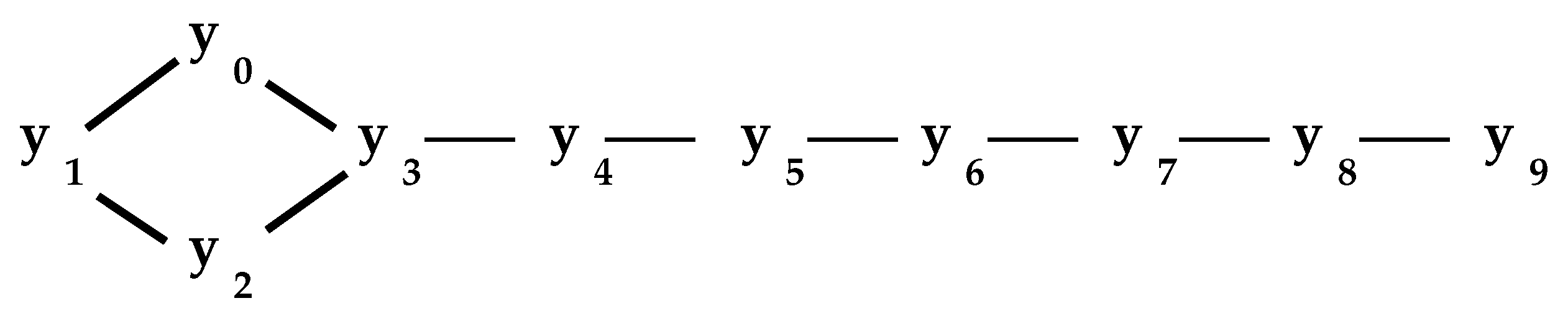
2. The Interior

Let S be a set. An operator $\tau :2^S\to 2^S$ is an injective function which maps subsets of S into subsets of S. We denote operators by Greek letters and use postfix notation, as in $Y.\tau$, where $Y\subseteq S$. An operator $\phi$ is said to be a closure operator if, for all $X,Y\subseteq S$, (C1) $Y\subseteq Y.\phi$ (expansive), (C2) $X\subseteq Y$ implies $X.\phi \subseteq Y.\phi$ (monotone) and (C3) $Y.\phi .\phi =Y.\phi$ (idempotent). Closure operators are a staple of topological mathematics.

If we replace axiom C1 with an contractive axiom I1, so that for all $X,Y\in \mathcal{S}$: (I1) $Y.\iota \subseteq Y$ (contractive); (I2) $X\subseteq Y$ implies $X.\iota \subseteq Y.\iota$ (monotone); and (I3) $Y.\iota .\iota =Y.\iota$ (idempotent), then $\iota$ is said to be an interior operator. We use $\iota$ to denote interior operators and $\phi$ to denote closure operators; they are similar, except that one is contractive while the other is expansive.

If one visualizes S as a polytope, then its closure might be the smallest sphere containing $\mathcal{S}$ (often called its convex hull), while its interior could be the largest inscribed sphere, or ball. Alternatively, if one thinks of S as being a bit of irregular surface terrain with ridges and valleys, then a closure operator fills in the valleys until the terrain is uniformly smooth. An interior operator, in contrast, levels the peaks and ridges until a smooth terrain is obtained.

Let $\mathcal{N}$ be a network. For any $Y\subseteq N$, we say the neighborhood of Y is $Y.\eta =\left\{z\right|\exists y\in Y,\{y,z\}\in L\}\cup Y$. (In graph theory, $Y.\eta$ is sometimes called the “closed neighborhood” of Y, and denoted $N\left[Y\right]$, while $N\left(Y\right)=Y.\eta -Y$ is called the “open neighborhood” [1,2]). Finally, since all operators map sets into sets, even when we are talking about the neighborhood of a single node, for example z in (1) below, we express it as $\left\{z\right\}.\eta$. A neighborhood closure operator, ${\phi }_{\eta }$, on $\mathcal{N}$ can be defined by

$$Y.{\phi }_{\eta }=\{z\in Y.\eta |\left\{z\right\}.\eta \subseteq Y.\eta \}.$$

(1)

$Y\subseteq Y.{\phi }_{\eta }\subseteq Y.\eta$, so ${\phi }_{\eta }$ is expansive. It is not hard to see that ${\phi }_{\eta }$ is monotone. Finally, since $Y.{\phi }_{\eta }\subseteq Y.\eta$, $Y.{\phi }_{\eta }$ must be idempotent, implying ${\phi }_{\eta }$ is a closure operator. (C3, or idempotency, is normally the most difficult property to prove when establishing a closure, or interior, operator.) The neighborhood closure operator, ${\phi }_{\eta }$, is fundamental to the development of following sections.

2.1. The Network Interior

Consider any node $y\in N$, and suppose there exists $z\in \left\{y\right\}.{\phi }_{\eta }$ implying $\left\{z\right\}.\eta \subseteq \left\{y\right\}.\eta$. Such a node, z whose “horizon” is contained in that of y, contributes very little to the information content of the network so that its removal from $\left\{y\right\}.\eta$ will result in little information loss. This node $z\in \left\{y\right\}.{\phi }_{\eta }$ can be reduced. The node y is irreducible if $\left\{y\right\}.{\phi }_{\eta }=\left\{y\right\}$. A sub-network, $\mathcal{I}\subseteq \mathcal{N}$, of irreducible nodes is called the network’s interior. In the remainder of this section we define an operator, $\omega$, which reduces any network to its irreducible core, and prove that it is almost an interior operator.

If $\left\{y\right\}$ is not closed, only elements z in $\left\{y\right\}.\eta$ could possibly be in $\left\{y\right\}.{\phi }_{\eta }$ so only those need be considered. If $\left\{z\right\}.\eta \subseteq \left\{y\right\}.\eta$ so that $z\in \left\{y\right\}.{\phi }_{\eta }$, we say z is subsumed by y, or z belongs to y. We can remove z from N, together with all its connections, and add z to $\left\{y\right\}.\beta$, the set of all nodes belonging to $\left\{y\right\}$. This set $\left\{y\right\}.\beta$ is called its $\beta$-set. Of course, $y\in \left\{y\right\}.\beta$. The cardinality $\left|\right\{y\}.\beta |$ is called its $\beta$-count.

The pseudocode reduce Pseudocode I was used to implement a process $\omega$ that reduces any network $\mathcal{N}$ to its irreducible core, $\mathcal{I}=\mathcal{N}.\omega$.

while there exist reduceable nodes {

reducible = 0

for_each {y} in N {

for_each {z} in {y}.nbhd - {y} {

if ({z}.nbhd contained_in {y}.nbhd {

// z is subsumed by y

remove z from network;

{y}.beta = {y}.beta union {z}.beta

reducible = 1 } } } }

Pseudocode I, $\omega$, reduce_network

Applied to ${\mathcal{N}}_1$, the well-known “Karate” network [6], this reduction code yields the interior depicted by bolder links in Figure 1.

Figure 1. The interior $\mathcal{I}$ of ${\mathcal{N}}_1$, the Karate network, is shown with bolder links.

In this figure, two nodes of the interior have been suffixed by “:n” to denote their $\beta$-count. Only nodes 1 and 33 have non-trivial $\beta$-sets of 12 and 8 elements, respectively, which have been delimited by dotted lines. (The $\beta$-set of node 33 might equally well have been the $\beta$-set of node 34; however, 33 precedes 34 in the reduction process).

Proposition 1.

The process ω described above is (I1) contractive and (I3) idempotent.

Proof. 

Readily, $\omega$ is contractive and it is idempotent because, when $\mathcal{I}=\mathcal{N}.\omega$ is irreducible, the loop is not executed, so $\mathcal{N}.\omega .\omega =\mathcal{I}=\mathcal{N}.\omega$.    □

One can show that $\mathcal{N}\subset {\mathcal{N}}^{\prime }$ need not imply that $\mathcal{N}.\omega \subset {\mathcal{N}}^{\prime }.\omega$, so $\omega$ is not an interior operator, even though we call $\mathcal{I}=\mathcal{N}.\omega$ the “interior”.

Proposition 2.

Let $\mathcal{I}=\mathcal{N}.\omega$ and ${\mathcal{I}}^{\prime }=\mathcal{N}.{\omega }^{\prime }$ be irreducible subsets of a finite network $\mathcal{N}$, then $\mathcal{I}\cong {\mathcal{I}}^{\prime }$.

Proof. 

Let $y_0\in \mathcal{I}$, $y_0\notin {\mathcal{I}}^{\prime }$. Then, $y_0$ belongs to some point $y_1$ in ${\mathcal{I}}^{\prime }$ and $y_1\notin \mathcal{I}$ else because $y_0.\eta \subseteq y_1.\eta$ implies $y_0\in \left\{y_1\right\}.\phi$ so $\mathcal{I}$ would not be irreducible.

Similarly, since $y_1\in {\mathcal{I}}^{\prime }$ and $y_1\notin \mathcal{I}$, there exists $y_2\in \mathcal{I}$ such that $y_1$ belongs to $y_2$. Now, we have two possible cases; either $y_2=y_0$, or not.

Suppose $y_2=y_0$ (which is often the case), then $y_0.\eta \subseteq y_1.\eta$ and $y_1.\eta \subseteq y_0.\eta$ or $y_0.\eta =y_1.\eta$. Hence, $i\left(y_0\right)=y_1$ is part of the desired isometry, i.

Now, suppose $y_2\ne y_0$. There exists $y_3\ne y_1\in {\mathcal{I}}^{\prime }$ such that $y_2.\eta \subseteq y_3.\eta$, and so forth. Since $\mathcal{I}$ is finite, this construction must halt with some $y_n$. The points $\{y_0,y_1,y_2,\cdots y_n\}$ constitute a complete graph $Y_n$ with $\left\{y_i\right\}.\eta =Y_n.\eta$, for $i\in [0,n]$. In any reduction, all $y_i\in Y_n$ reduce to a single point. All possibilities lead to mutually isomorphic maps.    □

Proposition 2 assures us that, even though which nodes are preserved in $\mathcal{I}$ is completely dependent on the order in $\omega$ that they are visited, the output must be effectively identical. For example, in Figure 2, assume the nodes x and z are irreducible elements of $\mathcal{I}$.

Figure 2. Equivalent nodes $y_i$ in an interior $\mathcal{I}$.

In each case, if $y_0\in \mathcal{I}$, then $y_1$ or $y_2$ could be as well. They are the equivalent nodes defining the isometry. Each set of equivalent nodes must be a “complete” subgraph of $\mathcal{N}$. (A graph, or network, K is said to be complete if for all $x,y\in K$, there is a link $\{x,y\}$. A complete graph on n nodes is denoted by $K_n$.)

A sequence, $\dot{\rho }=⟨y_0,\dots ,y_n⟩$ of $n+1$ nodes, where $\{y_{i-1},y_i\}\in L$, or a set of n links $\overline{\rho }=⟨\{y_0,y_1\},\dots ,\{y_{n-1},y_n\}⟩$ is called a path $\rho (y_0,y_n)$ of length n. It is often easier to describe a path in terms of its nodes, $\dot{\rho }$ rather than $\overline{\rho }$, which is more precise. By $\left|\rho \right(x,z\left)\right|$, we mean the length of the path independent of whether we are counting nodes or links.

A cycle $\dot{C}=⟨y_0,y_1,\dots ,y_n⟩$, where $y_n=y_0$, of length $n\ge 4$ is said to have a bridge if there exists a path $\overline{\rho }(y_i,y_k)\in L$ where $(k-i)mod\left(n\right)\ne 1$ [2]. If the path consists of a single link, it is called a chord. If C has no such chords, it is said to be a chordless cycle. Graphs, in which every cycle of length $\ge 4$ must have a chord, are called “chordal graphs” [7].)

Proposition 3.

The nodes of a chordless cycle are irreducible.

Proof. 

Let $\{y_{i-1},y_i\},\{y_i,y_{i+1}\}\in L$. Suppose $y_i\in y_{i-1}.{\phi }_{\eta }$ implying $y_{i+1}\in \left\{y_i\right\}.\eta \subseteq \left\{y_{i-1}\right\}.\eta$ or $\{y_{i+1},y_{i-1}\}\in L$ contradicting chordless assumption.    □

Proposition 4.

Let $\mathcal{N}$ be a finite network with $\mathcal{I}=\mathcal{N}.\omega$ being an irreducible subset. If $y\in \mathcal{I}$ is not an isolated point, then either:

   (1) there exists a chordless k-cycle $\dot{C}$, $k\ge 4$ such that $y\in \dot{C}$; or

   (2) there exist chordless k-cycles ${\dot{C}}_1,{\dot{C}}_2$ each of length $\ge 4$ with $x\in {\dot{C}}_1$ $z\in {\dot{C}}_2$ and y lies on a path from x to z.

Proof. 

Let $y_1\in \mathcal{I}$. Since $y_1$ is not isolated, let $y_0\in y_1.\eta$, so $\{y_0,y_1\}\in L$. $\ge 4$. Since $y_1$ is not subsumed by $y_0$, $\exists y_2\in y_1.\eta ,y_2\notin y_0.\eta$, and since $y_2$ is not subsumed by $y_1$, $\exists y_3\in y_2.\eta$, $y_3\notin y_1.\eta$. Since $y_2\notin y_0.\eta$, $y_3\ne y_0$.

Suppose $y_3\in y_0.\eta$, then $⟨y_0,y_1,y_2,y_3,y_0⟩$ constitutes a k-cycle $k\ge 4$, and we are done.

Suppose $y_3\notin y_0.\eta$. We repeat the same path extension. $y_3.\eta ⊈y_2.\eta$ implies $\exists y_4\in y_3.\eta$, $y_4\notin y_2.\eta$. If $y_4\in y_0.\eta$ or $y_4\in y_1.\eta$, we have the desired cycle. If not $\exists y_5,\dots$ and so forth. Because $\mathcal{N}$ is finite, this path extension must terminate with $y_k\in y_i.\eta$, where $0\le i\le n-3$, $n=\left|N\right|$.

The preceding establishes that any link sequence in $\mathcal{I}$ terminates in a cycle of length ≥4. Since $\mathcal{N}$ is symmetric, the link sequence could be extended in the opposite direction yielding (2).

Thus, if (1) is not the case, (2) must be.    □

The condition that y not be an isolated point is significant. Any tree structured network reduces to a single point, as do many networks consisting of triangles.

Corollary 1.

$\mathcal{N}$ is connected if and only if $\mathcal{I}$ is connected.

A collection of chordless cycles constitutes a cycle system which is itself a matroid [8] with a well defined rank [9]. If the network is projected onto a planar representation, then counting those cycles without a bridge yields the rank.

Figure 3 illustrates the interior of a small network on 21 nodes. It is a cycle system of rank 5. Here, the links of the interior have been made bolder and again its nodes have their $\beta$-counts appended.

Figure 3. A small network, ${\mathcal{N}}_2$, of 21 nodes. Interior links are bolder. $\beta$-sets are dotted.

The $\beta$-sets, such as $\{e$:$2\}.\beta$, are suggested by dotted lines. Note that this process effectively resolves the question of partitioning networks into disjoint communities [3,10,11], without having to specify the number of communities in advance, although some $\beta$-sets would have to be combined.

2.2. Reduction Performance

Technically, the $\omega$ process of Pseudocode I is $O\left(n^2\right)$ since it can achieve a worst case performance on the unbalanced network of Figure 4 provided the outer loop of the $\omega$ code of Pseudocode I encounters the nodes in order of their subscripts.

Figure 4. An unbalanced network.

Then, it will remove only one node on each iteration. However, in practice, $\omega$ appears to actually offer sub-linear performance. With networks of several thousand nodes, $\omega$ has never required more than seven iterations. For example, given the well-known Newman co-authorship network [12] of 363 persons with 823 connecting links, three iterations of the outer loop of the $\omega$ code of Pseudocode I reduces the network to 65 individuals with 111 links constituting its interior shown in Figure 5. (A fourth iteration is required to verify that there are no more reducible nodes.) The node Stauffer, in the upper left, has a $\beta$-set of 23 elements for which it may be regarded as a surrogate, and the lower left node Barabasi has a $\beta$-set of 41 elements. In the case of the Newman co-authorship network, the interior represents a significant reduction in the complexity of the network,

Figure 5. The interior $\mathcal{I}$ of ${\mathcal{N}}_3$, the 363 node co-authorship network of Newman [12].

3. Network Properties

There are several scalar properties associated with every network $\mathcal{N}$, including $n\_nodes=\left|N\right|$, $n\_links=\left|L\right|$ and $density=\left|L\right|/\left|N\right|$. The average node degree over all nodes is $2·density$, since every link has two end nodes [1,2]. These are trivial to calculate given N and L.

The number of triangles [13] embedded in $\mathcal{N}$ can be calculated by the count_triangles whose code is given in Pseudocode II.

k_total = 0

for_each link {x, z} in L {

MEET = {x}.nbhd meet {z}.nbhd

{x, z}.k_count = cardinality_of(MEET)

k_total = k_total + {x, z}.k_count }

n_triangles = k_total/3

Pseudocode II, count_triangles

Here, the $k\_count$ of a link denotes the number of triangles for which the link $\{x,z\}$ is one “side”. Since that triangle has three links, $n\_triangles=k\_total/3$. The computational cost of $\left\{x\right\}.nbhd\cap \left\{z\right\}.nbhd$ is essentially constant, so the cost of count_triangles is linear, or $O\left(L\right)$.

Other scalar properties are dependent on the concept of shortest paths. Let $x,z$ be two nodes in a connected network $\mathcal{N}$. Because $\mathcal{N}$ is connected, there exists a path $\rho (x,z)$ of length n. This may, or may not, be the shortest path (of minimal length) between them. We let $\sigma (x,z)$ denote the (or all) shortest path(s) between x and z. The path length $\left|\sigma \right(x,z\left)\right|$ is also known as the distance, $d(x,z)$, between x and y [1,2]. The $diameter\left(\mathcal{N}\right)$ of the network is the maximal distance, $d(x,z)$ for all $x,z\in N$. The $eccentricity$ of a node x is $e\left(x\right)=max\left(d\right(x,z\left)\right)$ for all $z\in N$. The $radius$, $r\left(\mathcal{N}\right)$, of the network is minimum eccentricity of any node y [2].

3.1. Communities

Many networks, especially those that represent social connections, are spotted with “clusters” of more densely connected nodes. These clusters of triangular links, which are often called communities, arise from the social phenomenon called triadic closure [14]. It is known that, in many social contexts, if x is connected to y and y is connected to z, then x is likely to be connected to z. Even though triadic closure is not really a closure operator, its principle has been identified on many repeated occasions [11,15]. (As normally encountered, triadic closure is not idempotent. Applied literally, the triadic closure of any network would be the complete graph/network on its n nodes).

However, we know of no formal definition as to what really constitutes a “community”.

There have been numerous efforts to identify communities in a network [16]. Several work on the principle of “bisection” in which removal of certain links separates the network into n distinct communities [10]. A common problem is that usually n must be designated in advance. Others iteratively partition the network, often using the Fiedler eigenvector [17]. Here, the question is when to stop the iteration.

A portion of the network that is dense with triangles may be regarded as a community. A connected sub-network of triangles is called a k-truss [18]. A connected subset of triangles could be tree-structured, so it is common to specify that a k-truss is a connected collection of links with a $k\_count>1$, where the $k\_count$ of a link $\{x,z\}$ is $\left|\right\{x\}.\eta \cap \{z\}.\eta |$ as in Pseudocode II. If $k\_count=2$, the Karate network of Figure 1 has just one 2-truss, consisting of links connecting the nodes {1, 2, 3, 4, 5, 6, 7, 8, 9, 11, 14, 30, 31, 33, 34} or just less than half the network. It has two 3-trusses connecting the nodes {1, 2, 3, 4, 8, 14} and {9, 24, 33, 34}. The small network of Figure 3 has two 2-trusses of links connecting the nodes {a, e, d, g, h, l, m, p, q, r, s} and {b, f, j, k, o} and four small 3-trusses, which are {b, j}, {d, g, l, m}, {p, q} and {r, s}. There are 23 2-trusses in the Newman network and each is large; however, there are only three 8-trusses. They are {Arenas, Dido-Guilera}, {Mano, Occaletti} and {Barabasi, Jeong, Oltavi, Raven, Schubert}; however, Arenas, Mano, Oltavi, Raven, and Schubert are not elements of the interior and thus not shown in Figure 5.

The larger values of the principal eigenvector of $A_{n\times n}$ (the adjacency matrix of the network) can indicate well-connected nodes, and often communities [3]. Nodes 1, 3, 33 and 34 of ${\mathcal{N}}_1$, the Karate network of Figure 1, dominate its principal eigenvector. The principal eigenvector of ${\mathcal{N}}_2$, the small network of Figure 3, are given in Table 2. Here, nodes $d,e,m,r$ stand out. Higher values in this eigenvector appear to correlate with higher node degree. The nodes $Barabasi$, $Jeong$ and $Oltvai$ (in $\left\{Jeong\right\}.\beta$) are most prominent in the eigenvector of the Newman network.

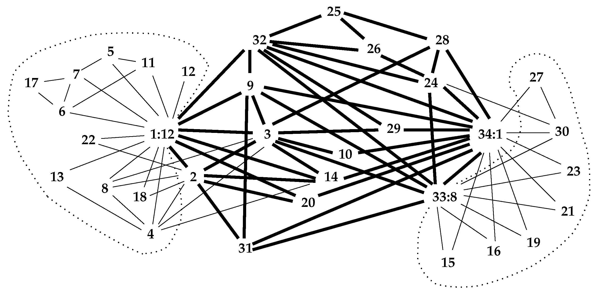
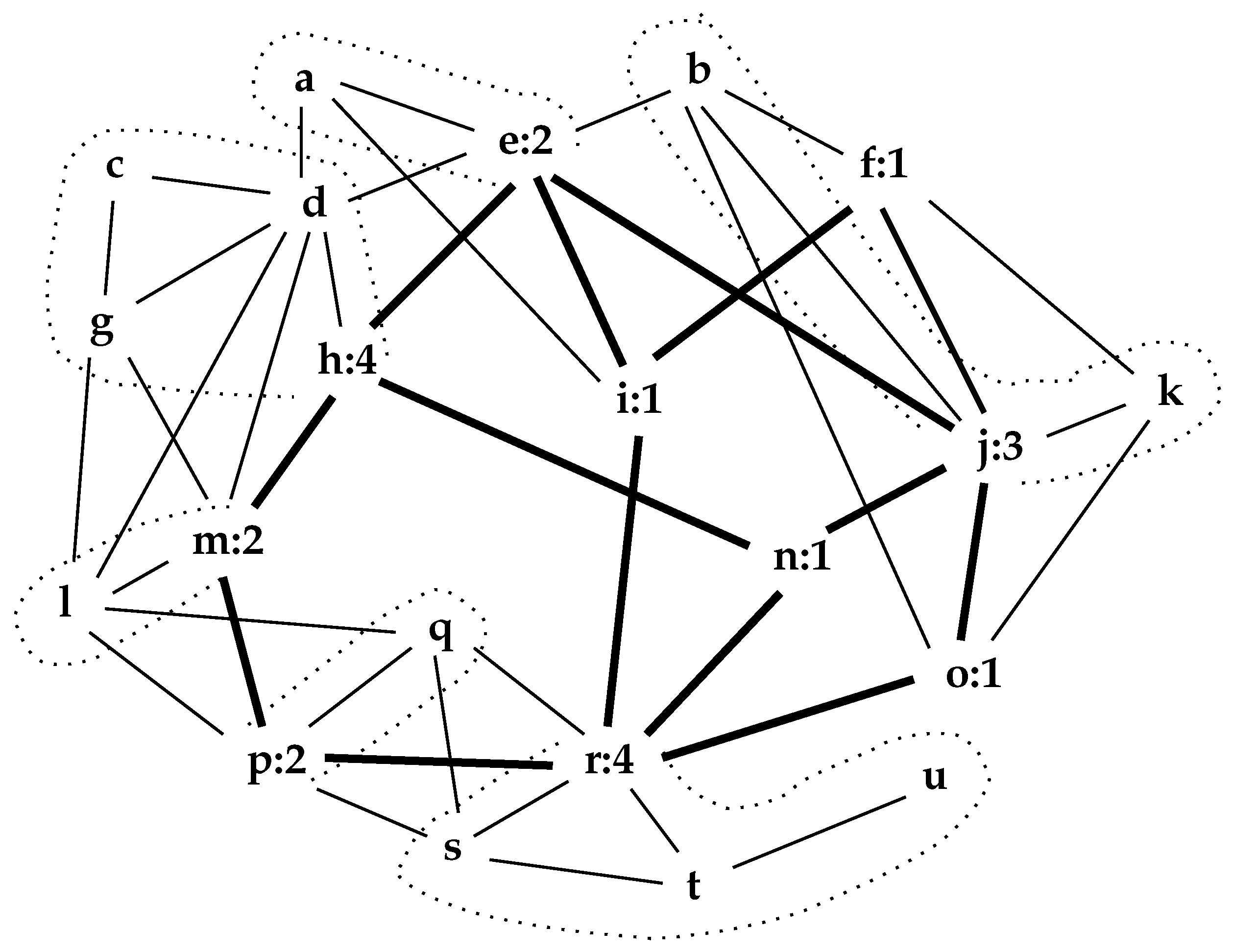
All of these methods have been proposed to denote “communities”. We would suggest that the $\beta$-sets attached to $\mathcal{I}$ also denote “communities”.

3.2. Important Nodes

A fundamental quest in the analysis of many networks is the identification of its “important” nodes. They may be a node of high degree in a community, but need not be. In social networks, “importance” may also be defined with respect to the path structure [19,20]. Those nodes, $C_d=\{y\in \mathcal{N}\}$ for which the eccentricity, $e\left(y\right)$, or ${\sum }_{x\ne y}d(x,y)$, is $minimal$, have traditionally been called the center of $\mathcal{N}$ [1,2]; they are “closest” to all other nodes. It is well known that this subset of nodes must be edge connected. One may assume that these nodes in the “center” of a network are “important” nodes.

Alternatively, one may consider those nodes which “connect” many other nodes, or clusters of nodes, to be the “important” ones. Let $ns{p}_{xz}\left(y\right)$ denote the number of shortest paths $\sigma (x,z)$ containing y; then, those nodes y for which $ns{p}_{xz}\left(y\right)$ is $maximal$ are involved in the most connections. Let $C_b=\{y\in \mathcal{N}\}$, for which $ns{p}_{xz}\left(y\right)$ is locally maximal. This is sometime called “betweenness centrality” [19,20,21]. (In [20], Newman proposed the notion of “random walk betweenness” as an alternative to shortest path betweenness).

3.3. Network Properties Preserved by the Interior

The next three lemmas, culminating in Proposition 5, help clarify the interaction of $\beta$-sets with the nodes of $\mathcal{I}$. In these lemmas, we assume that $x_0,y_0$ and $z_0\in \mathcal{I}$.

Lemma 1.

Let $y_k\in \left\{y_0\right\}.\beta$. There exists a node sequence $⟨y_0,y_1,\dots ,y_k⟩$ such that $y_i\in \left\{y_0\right\}.\beta$, $0\le i\le k$.

Proof. 

In the reduction process of Pseudocode I, if $y_{i+1}$ is subsumed by $y_i$, then $\left\{y_{i+1}\right\}.\beta \subset \left\{y_i\right\}.\beta$ yielding the chain of nested sets $\left\{y_k\right\}.\beta \subset \left\{y_{k-1}\right\}.\beta \subset \dots \subset \left\{y_0\right\}.\beta$.    □

Note that, even if $y_i\in \left\{y_{i-1}\right\}.\eta$ belongs to $y_{i-1}$, there may be other nodes $x_i\in \left\{y_{i-1}\right\}.\eta$ such that $x_i\notin \left\{y_{i-1}\right\}.\beta$.

Lemma 2.

Let $⟨y_0,\dots ,y_k⟩\in \left\{y_0\right\}.\beta$ and let $\{y_k,z\}\in L$ where $z\notin \left\{y_0\right\}.\beta$. Then, for all $y_i,0\le i\le k$, $\{y_i,z\}\in L$.

Proof. 

By the reduction process $\omega$, when $y_i$ is subsumed by $y_{i-1}$, $\left\{y_i\right\}.\eta \subseteq \left\{y_{i-1}\right\}.\eta$. Thus, if $\{y_i,z\}\in L$, then $z\in \left\{y_{i-1}\right\}.\eta$ or $\{y_{i-1},z\}\in L$.    □

Lemma 3.

Let $x\in \left\{x_0\right\}.\beta ,z\in \left\{z_0\right\}.\beta$ where $x_0,z_0\in \mathcal{I}$. If $\{x,z\}\in L$, then there exists $y\in \mathcal{I}$ such that $\{x,y\},\{y,z\}\in L$.

Proof. 

By Lemma 2, we know $\exists \{x,z_0\},\{z,x_0\}\in L$. If $\{x_0,y_0\}\in L,$ we are done. Thus, let us suppose not. By Proposition 4, we can assume $\exists y\in \mathcal{I}$ (or a sequence $y_i$) such that $\{x_0,y\},\{y,z_0\}\in L$. We claim $\{x,y\}\in L$, since otherwise $⟨y,x_0,\dots ,x,\dots ,z_0,y⟩$ is a chordless cycle of length $\ge 4$, and hence by Proposition 3 is irreducible. Similarly, $\{y,z_0\}\in L$.    □

Two $\beta$-sets, $\left\{x_0\right\}.\beta ,\left\{y_0\right\}.\beta$ are said to be $\beta$-connected if there exists $x,y\ne x_0,y_0$ where $x\in \left\{x_0\right\}.\beta$, $y\in \left\{y_0\right\}.\beta$ and $\{x,y\}\in L$. The preceding lemmas describe links that must exist if $\beta$-sets are connected. These are illustrated in Figure 6.

Figure 6. Links that can be inferred between connected $\beta$-sets.

In this figure, solid lines denote links that are “known” to exist for one reason or another. The dotted (⋯) lines that enclose $\beta$-sets were established by the reduction process. Each conforms to Lemma 1. Observe that the entire set of nodes, $\{x_1,x_2,z_1,z_2,z_3\}$ could constitute either $\left\{x_0\right\}.\beta$ or $\left\{z_0\right\}.\beta$ depending solely on the order of node reduction. This is illustrated in ${\mathcal{N}}_1$, Figure 1, where $\left\{33\right\}.\beta$ could have been $\left\{34\right\}.\beta$. Proposition 2 establishes that the structure of the interior, $\mathcal{I}$, is independent of the order in which nodes are encountered in the $\omega$ process; however, the structure of $\beta$-sets produced by the code reduce can be very dependent on this order.

The dashed links ( - - - ) denote links that can be inferred from Lemma 2. For instance, $z_1$ cannot subsume $z_2$ unless $x_1\in \left\{z_1\right\}.\eta$ because $x_1\in \left\{z_2\right\}.\eta$. The ( - $··$ - ) links connecting y to the nodes $x_1,z_1,z_2$ can be inferred from Proposition 3.

While in many networks the $\beta$-sets will be separated (as in Figure 3), they may be links between them. It is not hard to imagine a link between $a\in \left\{e\right\}.\beta$ and $c\in \left\{h\right\}.\beta$. The lemmas establish that either such a link must introduce a new chordless cycle into $\mathcal{I}$, or else there must be an abundance of “triangles” surrounding the network interior.

Proposition 5.

Let $\rho (x,z)$ be a path where $\{x,z\}\notin L$ ($i.e.,$$\left|\rho \right(x,z\left)\right|\ge 2$) and $x\in \left\{x_0\right\}.\beta$ and $z\notin \left\{x_0\right\}.\beta$. Then, there exists a path ${\rho }^{\prime }(x,y,z)$ where $y\in \mathcal{I}$ and $|{\rho }^{\prime }(x,y,z)|\le |\rho (x,z)|$.

Proof. 

We may assume that $\rho (x,z)\cup \mathcal{I}=\varnothing$, else there is nothing to prove. Thus, we may also assume that $\rho (x,z)$ lies entirely within connected $\beta$-sets. By Lemma 3, $\exists y\in \mathcal{I}$ such that $\{x,y\},\{y,z\}\in L$, so $|{\rho }^{\prime }(x,y,z)|=2\le |\rho (x,z)|$.    □

3.4. Network Centrality

Proposition 6.

If $\mathcal{N}$ is not unbalanced, then the center $C_d$ (in terms of distance) is an element of (or intersects with) the interior $\mathcal{I}$ of $\mathcal{N}$.

Proof. 

If x and z are in separated $\beta$-sets, then $\sigma (x,z)=⟨x=x_k,x_{k-1},\dots ,x_0⟩\cup ⟨y_1,\cdots ,y_m⟩\cup ⟨z_0,\dots ,z_n⟩$ where $y_1=x_0$, $y_m=z_0$ and $y_i\in \mathcal{I}$. Since $\mathcal{N}$ is not unbalanced, we may assume $k\approx n$, so the center of $\sigma (x,z)$ is one of the $y_1,\dots ,y_m$.

If x and z are in connected $\beta$-sets and $\left|\rho \right(x,z\left)\right|\ge 2$, then Proposition 5 establishes the existence of a shortest path through $\mathcal{I}$ as well.

If $x,z\in \left\{x\right\}.\beta$, then no shortest path involves $\mathcal{I}$; however, since $\mathcal{N}$ is not unbalanced, these constitute a small number of cases and can be ignored.    □

In Figure 2b, if $y_1$ is in the center C, then so are $y_0$ and $y_2$, implying $C\cap I\ne \varnothing$.

Proposition 6 requires that $\mathcal{N}$ not be too unbalanced. Figure 4 illustrates why. It is not hard to show that $y_5$ is the center with maximum distance over all x being $d(x,y_5)=4$. Our rule of thumb is that a network is reasonably well-balanced if, given any $x\in \left\{x_0\right\}.\beta$, then the probability that a randomly chosen y is also in $\left\{x_0\right\}.\beta$ is small, that is $pr(y\in \left\{x_0\right\}.\beta |x\in \left\{x_0\right\}.\beta )<\epsilon$ where $\epsilon <0.20$.

Proposition 7.

If $\mathcal{N}$ is not unbalanced, then any center $C_b$ of $\mathcal{N}$(in terms of betweenness) is an element of $\mathcal{I}$.

Proof. 

This proof follows the line of Proposition 6, in which, unless x and z are in the same $\beta$-set, all shortest paths $\sigma (x,z)$ either involve $\mathcal{I}$ or have a path ${\rho }^{\prime }(x,y,z)$ of the same length through $\mathcal{I}$. Hence, a node y for which ${\sigma }_{x,z}\left(y\right)$ is maximal will be an element of $\mathcal{I}$.    □

That $\mathcal{I}$ contains the betweenness center is evident in the Karate network of Figure 1 and the small network of Figure 3.

Figure 7 illustrates a somewhat different “unbalanced” network in which x and $z\notin \mathcal{I}$ are betweenness centers.

Figure 7. Another unbalanced network.

One can calculate that $nsp\left(x\right)=nsp\left(z\right)=6\ast 6+4\ast 6\ast 6+4\ast 6=204$ which are locally maximal.

Calculating betweenness centers is computationally expensive, even with improved algorithms (e.g., [21]). Knowing that they must exist in the interior $\mathcal{I}$ and restricting the calculation to just those nodes can greatly improve performance, especially when betweenness is employed in other procedures (e.g., [10]). Consequently, dwelling too much on unbalanced networks can be self defeating since the majority, and possibly almost all, networks are well-balanced.

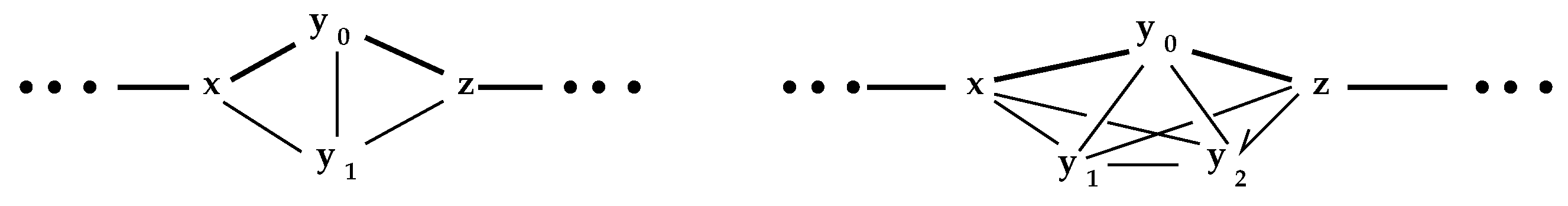
4. Network Generation by Expansion

The interior, $\mathcal{I}$, of a network $\mathcal{N}$ represents its global structure. If the $\beta$-count is appended to each node of $\mathcal{I}$, how well does $\mathcal{I}$ represent $\mathcal{N}$ as a whole? In effect, what is the information content of $\mathcal{I}$, so augmented?

One measure of the information content of any collection of network properties is the ability to construct, or generate, similar networks based on those properties. For example, given a network $\mathcal{N}=(N,L)$ one can construct many different networks ${\mathcal{N}}^{\prime }=(N^{\prime },L^{\prime })$ such that $|N^{\prime }|=|N|$ and $|L^{\prime }|=|L|$. However, they need not be at all similar to $\mathcal{N}$. Here, we are using “similar” in its colloquial sense. A formal notion of “similarity” would require it to be an equivalence relation. One way of determining the nature of networks with a given interior, $\mathcal{I}$, and known $\beta$-counts is to randomly generate some. Let $\mathcal{I}$ be given. Suppose the $\beta$-count of a node y is greater than one. New nodes can be attached to replace those of the original $\beta$-set. Let y:n be the node to be expanded ($n>1$) and let z denote the new node. Our code generates artificial node names of the form ‘A0, B0, …, Z0, A1, …’. The last generated node in the expansion of Figure 5 is $M11$. Besides the link $\{y,z\}$, we require $\left\{z\right\}.\eta \subseteq \left\{y\right\}.\eta$. A random number determines how many of the other nodes in $\left\{y\right\}.\eta$ will be linked to z, and which, if any, of those are also randomly chosen.

In the reduction process, $\omega$, nodes with considerable $\beta$-sets may be subsequently reduced themselves. In the re-expansion, a portion of the $\beta$-count of y may be transferred to the $\beta$-count of z. Pseudocode for a procedure expand to implement an operator $\epsilon$ that generates new nodes relative to the interior is given in Pseudocode III. ($\epsilon$, as shown here, is a round-robin procedure expanding one node in a $\beta$-set at a time. An alternative, and slightly faster, process can be found in [22]).

while still_expanding {

still_expanding = 0

for_each y in NODES {

if (y.beta_count > 1) {

z = new_node()

add new_node to NODES

chosen = choose_subset (y.nbhd)

// distribute some of y.beta_count to z

increment = y.beta_count/(n_chosen+1)

y.beta_count = y.beta_count - increment

z.beta_count = 1 + increment

add (y, z) to LINKS

// link z to chosen nodes in y.nbhd

for_each x in chosen {

add (x, z) to LINKS }

still_expanding = 1 } } }

Pseudocode III, $\epsilon$, expand_network

As a test, the interior $\mathcal{I}$ of ${\mathcal{N}}_2$, Figure 3, was expanded three times (using different random number seeds) to yield $exp.1$, $exp.2$ and $exp.3$ of Figure 8.

Figure 8. Three different expansions of $\mathcal{I}={\mathcal{N}}_2.\omega$, Figure 3.

Proposition 8.

Let $\mathcal{I}$ be the interior of a network $\mathcal{N}$, that is $\mathcal{I}=\mathcal{N}.\omega$, then $\mathcal{I}.\epsilon .\omega =\mathcal{I}$.

Proof. 

The expansion procedure of Pseudocode III was written to make this true. Consider $z_n$, the last node appended by $\epsilon$. By construction, $x_n.\eta \subseteq y_n.\eta$ for some $y_n$; thus, $z_n$ can be subsumed into $y_n.\beta$. A finite induction $z_n,\dots ,z_1$ completes the proof.    □

Considered as operators, $\epsilon$ is a left-inverse of $\omega$ since $\epsilon ·\omega =1$, where 1 denotes the identity operator. However, $\omega ·\epsilon \ne 1$, as shown by Figure 8.

To what extent are the network features of $\mathcal{N}$ enumerated in the preceding section preserved in the randomly generated networks, $\mathcal{N}.\omega .\epsilon$? Readily, the generation process $\epsilon$ was constrained so that $|\mathcal{N}.\omega .\epsilon |=\left|\mathcal{N}\right|$ and $\mathcal{N}.\omega .\epsilon .\omega =\mathcal{I}=\mathcal{N}.\omega$, thus the path-based centers of Section 3.4 are preserved. Some other network properties are illustrated in Table 1.

Table 1. Network properties of networks in Figure 8 generated from $\mathcal{I}={\mathcal{N}}_2.\omega$, Figure 3.

	$\left|\mathit{N}\right|$	$\left|\mathit{L}\right|$	$\mathbf{Density}$	$\mathit{Triangles}$	$2\_\mathit{Trusses}$	$3\_\mathit{Trusses}$
${\mathcal{N}}_2$	21	44	2.095	21	2	4
exp.1	21	49	2.333	31	1	3
exp.2	21	46	2.190	25	2	3
exp.3	21	37	1.762	13	2	2

Table 2 presents the principal eigenvector associated with the nodes of ${\mathcal{N}}_2$ in Figure 3 and for the three expansions shown in Figure 8. Note that, except for the ten nodes of $\mathcal{I}$, node values for generated expansions are not comparable with node values of the original $\mathcal{N}$.

Table 2. Value of nodes in Figure 3 and Figure 8 as expressed by the principal eigenvector.

	a	b	c	d	e	f	g	h	i	j	k
$\mathcal{N}$	0.179	0.182	0.123	0.350	0.293	0.155	0.226	0.234	0.194	0.231	0.120
	A0	B0	C0	D0	e	f	E0	h	i	j	F0
exp.1	0.170	0.295	0.225	0.033	0.355	0.129	0.053	0.306	0.202	0.265	0.162
exp.2	0.048	0.095	0.203	0.021	0.262	0.183	0.026	0.192	0.254	0.285	0.303
exp.3	0.125	0.212	0.056	0.187	0.265	0.120	0.093	0.353	0.270	0.243	0.195
	l	m	n	o	p	q	r	s	t	u
$\mathcal{N}$	0.291	0.293	0.159	0.174	0.271	0.220	0.280	0.187	0.104	0.022
	G0	m	n	o	p	H0	r	I0	J0	K0
exp.1	0.054	0.190	0.387	0.133	0.112	0.265	0.224	0.164	0.104	0.272
exp.2	0.192	0.118	0.379	0.271	0.142	0.253	0.325	0.307	0.017	0.115
exp.3	0.144	0.236	0.336	0.208	0.163	0.056	0.369	0.276	0.132	0.132

This section began with the question “how well does $\mathcal{I}$ represent $\mathcal{N}$ as a whole?” Figure 8 and Table 1 and Table 2 provide abundant evidence that, given just $\mathcal{I}$, with each node augmented with its $\beta$-count, a random process can generate new networks whose properties are very similar to those of $\mathcal{N}$. It would seem to be a very good description of $\mathcal{N}$.

5. Observations

This paper might have been titled “An Operator Approach to …” since the operators $\eta$, ${\phi }_{\eta }$, $\omega$ and $\epsilon$ play such an important role. This aspect is briefly suggested by Proposition 8, but not enlarged. However, surely, interesting networks are dynamic; they change over time which demands an operator approach. Thus, one might ask: “Is a transformation $\tau :\mathcal{N}\to {\mathcal{N}}^{\prime }$ continuous?” [23] The operators $\omega$ and $\epsilon$ are, in fact, “continuous” with respect to ${\phi }_{\eta }$. Moreover, it appears that $\mathcal{N}.\nu =\mathcal{N}-\mathcal{N}.\omega =\mathcal{N}-\mathcal{I}$ is a violator space in the sense of [24]. This could be expanded in the future.

However, computability is such a dominant theme in current network analysis and understanding that we thought focusing on the use of set-theoretic computer procedures such as reduce, count_triangles and expand was more important. Programming with set operators is not widespread. However, these set-theoretic procedures appear to be fast and quite scalable. The reduction, $\omega$, of the Newman co-authorship network to Figure 5 took 0.008 s; reduction of the smaller networks (Figure 1 and Figure 3) were each less than 0.001 s. Calculation of the eigenvectors of Figure 5 exceeded 5 s. Such anecdotal evidence is suggestive, but far from definitive.

Only standard set-theoretic reasoning was used to develop the reduction process, $\omega$, which leads to the concept of the “interior”, $\mathcal{I}$, of a network, $\mathcal{N}$, and its $\beta$-set. It is a powerful concept that effectively captures the essence of many networks, as shown by Section 4, in which very similar networks can be generated from $\mathcal{I}$ alone. Moreover, by reducing a network to its interior, one effectively partitions the network into it constituent $\beta$-set communities.

However, the reduction process has its limitations. Some networks are nearly irreducible to start with. The sparse network of Norwegian corporate directors [25] is an example. Hierarchical networks reduce to a single node, that is a single node interior with a very large $\beta$-set. Other networks can be too dense. The complete network $K_n$ also reduces to a single node. However, we believe that the easily computed interior is a most effective network descriptor and possibly should be an automatic first step in network description and understanding.

References

- Agnarsson, G.; Greenlaw, R. Graph Theory: Modeling, Applications and Algorithms; Prentice Hall: Upper Saddle River, NJ, USA, 2007. [Google Scholar]
- Harary, F. Graph Theory; Addison-Wesley: Reading, MA, USA, 1969. [Google Scholar]
- Newman, M.E.J. Finding community structure in networks using the eigenvectors of matrices. Phys. Rev. E 2006, 74, 1–22. [Google Scholar] [CrossRef] [PubMed]
- Newman, M. Networks; Oxford University Press: Oxford, UK, 2018. [Google Scholar]
- Orlandic, R.; Pfaltz, J.L.; Taylor, C. A Functional Database Representation of Large Sets of Objects. In Proceedings of the 25th Australasian Database Conference (ADC 2014), Brisbane, Australia, 14–16 July 2014; Wang, H., Saraf, M.A., Eds.; Springer: Cham, Switzerland, 2014; pp. 189–196. [Google Scholar]
- Zachary, W.W. An Information Flow Model for Conflict and Fission in Small groups. J. Anthropol. Res. 1977, 33, 452–473. [Google Scholar] [CrossRef]
- McKee, T.A. How Chordal Graphs Work. Bull. ICA 1993, 9, 27–39. [Google Scholar]
- White, N. Theory of Matroids; Cambridge University Press: Cambridge, UK, 1986. [Google Scholar]
- Pfaltz, J.L. Cycle Systems. Math. Appl. 2020, 9, 55–66. [Google Scholar] [CrossRef]
- Girvan, M.; Newman, M.E.J. Community structure in social and biological networks. Proc. Natl. Acad. Sci. USA 2002, 99, 7821–7826. [Google Scholar] [CrossRef]
- Newman, M.E.J. Detecting community structure in networks. Eur. Phys. J. B 2004, 38, 321–330. [Google Scholar] [CrossRef]
- Newman, M.E.J. The structure and function of complex networks. SIAM Rev. 2003, 45, 167–256. [Google Scholar] [CrossRef]
- Tsourakakis, C.E.; Drineas, P.; Michelakis, E.; Koutis, I.; Faloutos, C. Spectral counting of triangles via element-wise sparsification and triangle-based link recommendation. Soc. Netw. Anal. Min. 2011, 1, 75–81. [Google Scholar] [CrossRef]
- Mollenhorst, G.; Völker, B.; Flap, H. Shared contexts and triadic closure in core discussion networks. Soc. Netw. 2012, 34, 292–302. [Google Scholar] [CrossRef]
- Granovetter, M.S. The Strength of Weak Ties. Am. J. Sociol. 1973, 78, 1360–1380. [Google Scholar] [CrossRef]
- Newman, M.E.J. Modularity and community structure in networks. Proc. Natl. Acad. Sci. USA 2006, 103, 8577–8582. [Google Scholar] [CrossRef] [PubMed]
- Fiedler, M. Algebraic Connectivity of Graphs. Czechoslovak Math. J. 1973, 23, 298–305. [Google Scholar] [CrossRef]
- McCulloh, I.; Savas, O. k-Truss Network Community Detection. In Proceedings of the 2020 IEEE/ACM International Conference on Advances in Social Networks Analysis and Mining (ASONAM), The Hague, The Netherlands, 7–10 December 2020. [Google Scholar]
- Freeman, L.C. Centrality in Social Networks, Conceptual Clarification. Soc. Netw. 1978, 1, 215–239. [Google Scholar] [CrossRef]
- Newman, M.E.J. A measure of betweenness centrality based on random walks. Soc. Netw. 2005, 27, 39–45. [Google Scholar] [CrossRef]
- Brandes, U. A Faster Algorithm for Betweeness Centrality. J. Math. Sociol. 2001, 25, 163–177. [Google Scholar] [CrossRef]
- Pfaltz, J.L. Computational Processes that Appear to Model Human Memory. In Proceedings of the 4th International Conference, Algorithms for Computational Biology (AlCoB 2017), Aveiro, Portugal, 5–6 June 2017; pp. 85–99. [Google Scholar]
- Pfaltz, J.; Šlapal, J. Transformations of discrete closure systems. Acta Math. Hung. 2013, 138, 386–405. [Google Scholar] [CrossRef]
- Kempner, Y.; Levit, V.E. Violator spaces vs closure spaces. Eur. J. Comb. 2019, 80, 203–213. [Google Scholar] [CrossRef]
- Seierstad, C.; Opsahl, T. For the few not the many? The effects of affirmative action on presence, prominence, and social capital of female directors in Norway. Scand. J. Manag. 2011, 27, 44–54. [Google Scholar] [CrossRef]