Abstract
HIFUN is a high-level query language for expressing analytic queries of big datasets, offering a clear separation between the conceptual layer, where analytic queries are defined independently of the nature and location of data, and the physical layer, where queries are evaluated. In this paper, we present a methodology based on the HIFUN language, and the corresponding algorithms for the incremental evaluation of continuous queries. In essence, our approach is able to process the most recent data batch by exploiting already computed information, without requiring the evaluation of the query over the complete dataset. We present the generic algorithm which we translated to both SQL and MapReduce using SPARK; it implements various query rewriting methods. We demonstrate the effectiveness of our approach in temrs of query answering efficiency. Finally, we show that by exploiting the formal query rewriting methods of HIFUN, we can further reduce the computational cost, adding another layer of query optimization to our implementation.
1. Introduction
Data emanating from high-speed streams are prevalent everywhere in today’s data eco-system. Examples of data streams include IoT data [1], data series [2], network traffic data [3], financial tickers [4], health care transactions [5,6], the Linked Open Cloud [7,8] and so on. In order to extract knowledge and find useful patterns [9,10], these data need to be rapidly analyzed and processed. However, this is a challenge, as new data batches arrive continuously at high speed, and efficient data processing algorithms are needed.
The research community has already provided open-source and commercial distributed batch processing systems such as Hadoop [11], MapReduce [12] and Oracle Cloud Infrastructure [13], that allow query processing over static and historical datasets, enabling scalable parallel analytics. However, even with those technologies, processing and analyzing large volumes of data is not efficient enough. This is true especially in scenarios that need rapid responses to change over continuous (big) data streams [14]. Consequently, stream processing has gained significant attention. Several streaming engines, including Spark Streaming [15], Spark Structured Streaming [16], Storm [17], Flink [18] and Google Data Flow [19], have been developed to that purpose.
Current research mainly focuses data stream management systems processing continuous queries over traditional data streams [20], or massive amounts of spatio-temporal data that are increasingly being collected and stored. Most of the existing methodologies have been devised to store all the incoming data on distributed storage [21], and others [22,23] use complex indexing techniques to increase the performance from the data access point of view. However, such approaches are untenable in real world problems, and continuous query processing techniques have been developed to overcome this limitation by utilizing the storage space to produce results in an incremental fashion rather than aiming to process all the available data [24,25].
Continuous query processing is a major challenge in a streaming context. A continuous query is a query which is evaluated automatically and periodically over a dataset that changes over time [26], and allows the user to retrieve new results from a dataset without the need to issue the same query repeatedly. The results of continuous queries are usually fed to dashboards, in large enterprises, to provide support in the decision-making process [27]. In addition, besides their ever increasing volume, datasets change frequently, and as such, results to continuous queries have to be updated at short intervals.
Motivation and Contributions
As new data are constantly arriving at a high rate, datasets are growing rapidly, and the re-evaluations of queries are incurring delays. The problem on which we focus in this work is incremental query evaluation; that is, given the answer to a given query at time t, on dataset D, how can one find the answer to the same query at time on dataset , assuming that the answer at time t has been saved andthe results become stale and stagnant over time. Incremental processing is an auspicious approach for refreshing mining results, as it uses previously saved results to avoid the cost of re-computation from scratch. There is an obvious relationship between continuous queries and materialized views [28], since a materialized view is a derived database relation whose contents are periodically updated by either a complete or an incremental refresh based on a query. Incremental view maintenance methods [29] exploit differential algorithms to re-evaluate the view expression in order to enable the incremental updating of materialized views. However, in our case, although the target was the same, the methods used were different: we devised an algorithm for incremental processing of continuous queries that processes only the most recent data partition and exploits already computed information, without requiring evaluating the query over the entire dataset.
In this paper, we study this problem in the context of HIFUN, a recently proposed high-level functional language of analytic queries [30,31]. Two distinctive features of HIFUN are that (a) analytic queries and their answers are defined and studied in the abstract, independently of the structure and location of the data, and (b) each HIFUN query can be mapped either to an SQL group-by query or to a MapReduce job. HIFUN separates the conceptual and the physical levels so that one can express analysis tasks as queries at the conceptual level independently of how their evaluations are done at the physical level using existing mechanisms (e.g., SQL engines, Graph engines or MapReduce) which perform the actual evaluation of queries. In [32], the authors investigated how HIFUN can be used for easing the formulation of analytic queries over RDF data. In this works we focus on relational and unstructured data. For example, if the data reside in a relational database, then the mapping mechanism can use SQL in order to evaluate the conceptual query, whereas if the data are unstructured, then mapping mechanisms need to be algorithms specialized to the evaluation based on MapReduce programming model. Our approach exploits the Spark Streaming and the Spark Structured Streaming in the physical layer to implement an incremental evaluation algorithm using HIFUN semantics.
An initial approach in this direction has already been presented in a workshop [33], focusing on incrementally updating continuous query results, preventing the costly recomputation from scratch. Based on those ideas, in this paper, we exploit complex rewritings at the physical layer in order to further minimize the evaluation cost.
More specifically, the contributions of this paper are as follows:
- We use the HIFUN language to define the continuous query problem and give a high-level generic algorithm for its solution.
- Then we map the generic algorithm to the physical level, implementing the evaluation mechanism both as SQL queries and MapReduce tasks.
- Further, we show how HIFUN query rewriting can be implemented in the physical layer.
- Finally, we experimentally show that our implementation provides considerable benefits in terms of efficiency.
Although an incremental evaluation of queries based on the HIFUN language was already published [33], and although similar rewritings have been used extensively on relational databases [34], this is the first time that similar rewritings have been proposed for the HIFUN functional language. In addition, they are not trivially implemented either. In this paper, besides the functional layer, we also show how to implement it in two completely different physical setups. The remainder of the paper is organized as follows. In Section 2, we present related work, and in Section 3 the theoretical framework and the query language model used. Then in Section 4, we describe our algorithms for incremental evaluations of continuous queries at the HIFUN level, and in Section 5, the corresponding implementation at the physical level. In Section 6, we present an evaluation of our system, and finally, in Section 6, we conclude the paper and discuss possible directions for future work.
2. Related Work
To respond to the intensive computational requirements of massive dataset analysis, a number of frameworks are already available in the literature that deal with continuous queries such as Spark Streaming and Flink [35]. Continuous queries were introduced for the first time in the TQL language in Tapestry [36], for content-based filtering of an append-only email and message posting database. Conceptually, a restricted subset of the SQL was used, and it was converted into an incremental query that was defined to retrieve all answers obtained in an interval of t seconds. The incremental query was issued continuously, every t seconds, and the union of answers returned constituted the answer to the continuous query. An incremental evaluation approach was used, to avoid the repetitive computations and to return only the new results to the users. Besides this, other architectures have been proposed as well to process continuous queries, such as the NiagaraCQ [37] and the OpenCQ [38]. Both systems use continuous queries over changing data, similarly to Tapestry, periodically executing individual queries. However, all aforementioned approaches focus on relational databases and thus do not deal with issues that appear when moving to semi- and unstructured data.
STREAM [26] is an all-purpose framework that focuses on addressing the demands imposed by data streams on data management. The authors pay attention to memory management in order to enable approximate query answering. In particular, one of the project’s goals is to understand how to efficiently run queries given a bounded amount of memory. The system can process streaming data, but it is designed as a centralized system.
Our approach is a coherent integration of Apache Spark, as a computational engine, with semantics of HIFUN that can be used to rewrite continuous queries for optimization. Spark can tackle different paradigms (e.g., structured and unstructured processing) based on a common set of abstractions. The data itself can be stored in a centralized or distributed manner with different data models (e.g., relational and unstructured sources). In other words, HIFUN queries are agnostic to the evaluation layer and the nature and location of the data.
3. Preliminaries—The HIFUN Query Language
In this section, we describe briefly the conceptual model of the HIFUN language. For further details on the HIFUN language, the interested reader is referred to some relevant papers [30,31].
The basic notion used in defining HIFUN is that of an of a dataset. In HIFUN, each attribute is seen as a function of the dataset for some domain of values. For example, if the dataset D is a set of tweets, then the attribute “character count” (denoted as cc) is seen as a function , such that, for each tweet t, is the number of characters in t.
Next we provide an example that we will use throughout the paper. Consider a distribution center (e.g., Walmart) which delivers products of various types in a number of branches, and suppose that D is the set of all delivery invoices collected over a year. Each delivery invoice has an identifier (e.g., an integer) and shows the date of delivery, the branch in which the delivery took place, the type of product delivered (e.g., CocaLight) and the quantity (i.e., the number of units delivered of that type of product). There is a separate invoice for each type of product delivered; and the data on all invoices during the year are stored in a data warehouse for analysis purposes. The information provided by each invoice would most likely be represented as a record with the following fields: invoice number, date, branch, product and quantity. In the HIFUN approach, this information is seen as a set of four functions, namely, d, b, p and q, as shown in Figure 1, where D stands for the set of all invoice numbers and the arrows represent attributes of D. Following this view, given an invoice number, the function d returns a date, the function b a branch, the function p a product type and the function q a quantity (i.e., the number of units of that product type).
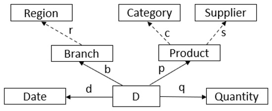
Figure 1.
Running example.
Assume now that we want to know the total quantity delivered to each branch (during the year); call this query Q. Its evaluation needs the extensions of only two among the four functions, namely, b and q. Figure 2a shows a toy example, where the dataset D consists of seven invoices, numbered 1 to 7. It also shows the values of the functions b and q, for example, , , and so on; and , , and so on.
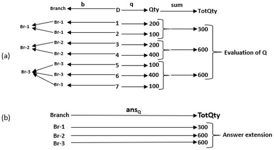
Figure 2.
An analytic query (a) and its answer (b).
In order to find the answer to query Q, for each branch , we proceed in three steps as follows:
- Grouping. Group together all invoices j of D such that .
- Measuring. Apply q to each invoice j of the -group to find the corresponding quantity .
- Aggregation. Sum up the s thus obtained to get a single value .
This process creates a function associating each branch with a value , as shown in Figure 2b. We view the ordered triple as a query, the function as the answer to Q and the computations described above as the query evaluation process. The function b that appears first in the triple and is used in the grouping step is called the grouping function; the function q that appears second in the triple is called the measuring function; and the function that appears third in the triple is called the reduction operation (or the aggregate operation).
3.1. Analysis Context
Now, the attributes d, b, p and q of our running example are “factual” or “direct” attributes of D in the sense that their values appear on the delivery invoices. However, apart from these attributes, analysts might be interested in attributes that are not direct but can be “derived” from the direct attributes. Figure 1 shows the direct attributes together with several derived attributes: attribute r can be derived from attribute b based on geographical information on the location of each branch; and attributes s and c can be derived from a product’s master table. The set of all attributes (direct and derived) that are of interest to a group of analysts is called an analysis context (or simply a context).
Actually, as we shall see shortly, the context is the interface between the analyst and the dataset, in the sense that the analyst uses attributes of the context in order to formulate queries (in the form of triples, as seen earlier). The users of a context can combine attributes to form complex grouping functions.
In HIFUN one can form complex grouping or measuring functions using the following three operations on functions: composition, pairing and Cartesian product projection. An example is shown in Figure 2. As shown, in order to ask for the total quantities by region, we need to use the composition as a grouping function in order to express the query: . The attribute r is derived, as the value can be computed from this of attribute b (e.g., from a specific branch name one can derive the region in which the branch exists). For pairing, in order to ask for a total quantities delivered by a branch product, we need to use the pairing ∧ operator as a grouping function in order to express the query: (e.g., its answer associates every pair (branch, product) with a total quantity). We assume now that the query has been evaluated and its results stored in a cache. Then we can compute the totals by branch and the totals by product from the result of Q, using the following rewritings:
3.2. Query Rewriting
Independently of how a given query is evaluated, the formal model of HIFUN supports query rewriting. An incoming query or a set of queries can be rewritten at the conceptual level, in terms of other queries to reduce the evaluation cost.
Common Grouping and Measuring Rewriting Rule (CGMRR): Let be a set of n queries with the same grouping function and the same measuring function, but possible different reduction operations. In this case the rewriting of Q is the following: , meaning that the grouping and the measuring steps are done only once and the n reduction operations are applied to the measuring results.
Common Grouping Rewriting Rule (CGRR): Let be a set of n queries with the same grouping function but possibly different measuring and reduction operations. In this case the rewriting of Q is the following: , meaning that the grouping is done only once and the n measuring and reduction steps are applied to the results of grouping.
Common Measuring and Operation Rewriting Rule (CMORR): Let be a set of n queries with the same measuring function and the same reduction operation, but possibly different grouping functions. In this case the rewriting of Q is the following: , where denotes the domain of definition of . This rewriting rule is derived from the following basic rewriting rule of the HIUN Language [30,31]:
Basic Rewriting Rule (BRR): Let and . Then Q can be rewritten as follows: under the assumption that the operation is distributive.
A more concise expression of this rule is the following: , which can be read as: evaluate first the “inner” query ; then use its answer as the measuring function to evaluate the “outer” query .
4. Methods
4.1. Incremental Computation in HIFUN
In this section, we show how we can use HIFUN language to incrementally evaluate continuous queries. An important common feature of real-life applications is that the input data continuously grow and old data remain intact. As such, for the rest of this paper we assume that the dataset being processed can only increase in size between t and . In such a scenario, the idea of incrementally evaluating a continuous query is to use the results of an already performed computation on the old data, and evaluate the query only on the data appended between t and ; eventually new and previous results should be merged.
As we saw earlier, in an HIFUN query , the domain of the definition of an answer coincides with the range of the grouping function. Consider, for instance, the query of our running example, asking for the totals by branch. The domain of the answer is the set of all branches and this set is also the range of b. We call this set the key of the query. Now, in a continuous query, the key might change over time. Indeed, in the case of totals by branch, new branches might start operation between t and , whereas branches operating at time t might cease to operate between t and .
Figure 3 illustrates our incremental approach for continuous queries—the same query asked two times. We perceive the problem of incremental evaluation as follows: let be the answer of continuous query Q at time t, on dataset D; let be the answer of Q at time on dataset , where ; and let be the answer of Q at time on dataset . Moreover, let K be the key of Q at time t and let be the key of Q at time .
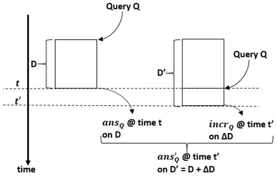
Figure 3.
Incremental computing over an append-only dataset.
Our algorithm for computing supports both distributive and non-distributive operations. Without loss of generality, we present in the sequel four cases of distributive operations and a non-distributive one:
- op= sum: if i is in ;if i is in ; if i is in ;
- op= min: if i is in ; if i is in ; if i is in ;
- op= max: if i is in ; if i is in ; if i is in ;
- op= count: if i is in ; if i is in ; if i is in ;
The non-distributive aggregate operation of the average can be computed by applying a combination of distributive aggregate operations. More specifically, the answer of query Q at time is computed as follows:
- op = avg:
- -
- if i is in ;
- -
- if i is in ;
- -
- if i is in ;
Distributive aggregate operations are those whose computation can be distributed and be recombined using the distributed aggregates. All operations , , and are distributive. This means that if the data are distributed into n sets, and we apply the aforementioned distributive operation to each one of them (resulting in n aggregate values), the total aggregate operation can be computed for all data by applying the aggregate operation for each subset and then combining the results. For example: . We also support the non-distributive aggregate operation: . Non-distributive aggregate operations can be computed by algebraic functions that are obtained by applying a combination of distributive aggregate functions. For example, the average can be computed by summing a group of numbers and then dividing by the count of those numbers. Both sum and count are distributive operations.
4.2. System Implementation
As already mentioned, HIFUN queries can be defined at the conceptual level independent of the nature and the location of the data. These queries can be evaluated by encoding them either as MapReduce jobs or SQL group-by queries, depending on the nature of the available data. Two different physical-level mechanisms are used to physically evaluate HIFUN queries over live data streams: (1) Spark Streaming [15] and (2) Spark Structured Streaming [16]. Both mechanisms support the micro-batching concept—fragmentation of the stream as a sequence of small batch chunks of data. On small intervals, the incoming stream is packed to a chunk of data and is delivered to the system to be further processed. This system is based on definitions and features as formally proposed by HIFUN, and performs optimizations through incremental approach and query rewritings to reduce the computational costs.
4.2.1. Continuous HIFUN Queries over Micro-Batches
In the micro-batching approach, as a dataset continuously grows and as new data become available, we process the tuples in discrete batches. The batches are processed according to a particular sequence. As a high volume of tuples can be processed per micro-batch, the aforementioned mechanism uses parallelization to speed up data processing. An initial dataset is followed by a continuous stream of incremental batches that arrive at consecutive time intervals . As we already explained, incremental evaluation would produce the query results at time by simply combining the query results at time t with the results from processing the incremental batches . Two key observations should be made here. The first is that computations needed are solely performed within the specific batch, following the evaluation scheme described in the previous section. Therefore, for every batch interval we calculate a result based on delta subset , e.g., . The second observation is that the state should be kept across all batches to perform in-memory computations by wrapping the accessed data as distributive data collections. After the evaluation of each query is completed for each micro-batch, we need to keep the states across all batches. The previous state value and the current delta result are merged together, and the system produces a new state incrementally, e.g., . Figure 4 illustrates this incremental approach.
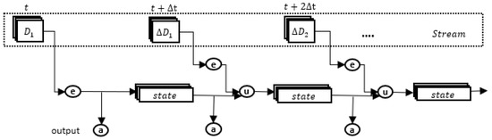
Figure 4.
State maintenance.
4.2.2. Continuous HIFUN Queries Using MapReduce
The abstract definition of a query evaluation is implemented on the physical level using the MapReduce programming model exploiting Spark Streaming. Spark Streaming is a stream processing framework based on the concept of discretized streams and provides the DStream API, which accepts sequences of data which arrive over time. The API implements the micro-batch stream processing approach with periodic checking of internal state at each batch interval. Internally, each DStream is represented as a sequence of data structure called resilient distributed datasets (RDDs) which keeps the data in memory as they arrive in each batch interval.
Generic Evaluation Schema to MapReduce. In this section, we elaborate on the generic query evaluation schema, described in Section 3, by presenting details of its implementation in the physical layer when Spark Streaming and the MapReduce programming model are sed:
- (a)
- Query Input Preparation. A set of attributes which are included in grouping and measuring part of Q is used to extract the information from the initial unstructured dataset. A map function is used that applies the given attributes to each record of the initial DStream and returns a new DStream which contains the information useful for the next evaluation steps.
- (b)
- Grouping Partition Construction. In this step, a map function constructs the grouping partition as follows. The mapper receives the tuples created from the previous step and extracts the key–value pairs. The result is a new PairDStream in which the key K is the value of the grouping attribute of each data item or the value of the grouping attributes if the domain of is the Cartesian product of two or more grouping attributes. The value V is the value of the measuring attribute of each data item.
- (c)
- Grouping Partition Reduction. In this step a reduce function is used to merge the values of each key using a query operation , and a new DStream is created as the query answer of the current micro-batch.
Rewritings to MapReduce As already described, a set Q can be rewritten according to certain rewriting rules. In this subsection, we give a detailed description how the evaluation mechanism leverages these rules.
Common Grouping and Measuring Rewriting Rule. In this case of rewriting, n different operations are applied to the common grouping and measuring attributes. In the Query Input Preparation step the information is extracted from the initial unstructured dataset using the common grouping and measuring attributes, which appear in the query set Q. A map function is used to apply the given common attributes to each record of the initial DStream and returns a new DStream containing the values of the common grouping and measuring attributes for each record. This is useful for the following evaluation steps. As a next evaluation step, a map function constructs the grouping partition as follows. The mapper receives the tuples created from the previous step and emits key–value pairs , where K is the value of the common grouping attribute for each tuple and value V is synthetic and carries a list of measuring attribute values. The measuring value of each tuple is used and repeated n times to create a list of n values assigned to the key K. The length n of the list depends on the number of the operations which appear in the query set Q. As a final evaluation step, the reduction of the grouping partition is needed. A reduce function merges the n values for each key, using the n operations included in the rewritten set, and produces the query answer in the form of key–value pairs , where is the key of the query, and its synthetic value containing the reduced value for each operation applicable to the measuring attribute. The answer of the Common Grouping and Measuring Rewriting Rule is completed when a set of is created.
Common Grouping Rewriting Rule. The evaluation of this rewriting rule is slightly different to the evaluation of the Common Grouping and Measuring Rewriting Rule. In this case n different measuring attributes are reduced to the common grouping attribute, applying n possible different operations. In the Query Input Preparation step, the information is extracted from the initial unstructured dataset using the common grouping and the n different measuring attributes which appear in the query set Q. A mapping function is used to apply the given common grouping attribute and the n measuring attributes to each record of the initial DStream. It then returns a new DStream, containing the values of the common grouping and measuring attributes for each record, useful for the next evaluation steps. As a next evaluation step, a map function constructs the grouping partition as follows: The mapper receives the tuples created from the previous step and emits the key–value pairs , where K is the value of the common grouping attribute for each tuple and the value V is synthetic, and carries a list of n measuring attribute values. The length n of the list depends on the number of the measuring attributes which appear in the query set Q. As the final evaluation step, the Grouping Partition Reduction is performed as follows: The reduce function applies for each key K, the n operations on the list of n values and produces the query answer in the form of key–value pairs , where is the query key and its synthetic value containing the reduced value for each operation applicable to the measuring attributes. The answer of the Common Grouping Rewriting Rule is completed when a set of is created.
Common Measuring and Operation Rewriting Rule. In this rule, the same measuring attribute and the same operation are associated with the n grouping attributes. The evaluation of the base query is first required as described in the generic evaluation schema, and produces an intermediate result required to the evaluation of the projection queries. The intermediate result is produced in the form of key–value pairs , where is the key of the base query and its reduced value. For each projection query, a map function receives the pair tuples of the intermediate result and a MapReduce job constructs the answer as follows: In the Grouping Partition Construction step a mapper emits key–value pairs , where the key is emitted as the value of the subset of the key , which is specified by the projection operation, and the value is emitted as a new value assigned to . Finally, to perform the Grouping Partition Reduction step, the reduce function is applied and produces the answer for each projection query in the form of key–value pairs , where is the query key and its value. The final answer of this rule is completed when n sets of are created.
Basic Rewriting Rule. The evaluation of the base query is required first as described in the generic evaluation schema, and produces an intermediate result of the “inner” query required for the evaluation of the “outer” query. The intermediate result is produced in the form of key–value pairs , where is the key of the base query and its value. A set of key–value pairs is available for the evaluation of the “outer” query as follows. A map function receives the key–value pair of the intermediate result and constructs a new set of the key–value pairs as follows. For each key a new key is emitted, specified by the association between and as defined in the context. The value is emitted as a new value for the key . Finally, a reducing function is applied and produces the answer of the “outer” query in the form of key–value pairs , where is the query key and its value.
Incremental Evaluation
We have to note that we maintain the state across the micro-batches (using the mapWithState method), using the key–value pairs produced for each micro-batch. Stateful transformation is a particular property used in this case, and it enables us to maintain the state between the various micro-batches across a period of time. That operation is able to execute partial updates for only the newly arrived keys in the current micro-batch. As such, computations are initiated only for the records that need to be updated. The state information is stored as a mapWithStateRDD, thereby benefiting from the distribution’s effectiveness of Spark.
Next we focus on how the incremental update mechanism leverages the rewriting rules and allows updating the state(s) between the micro-batches using the MapReduce programming model. We distinguish the incrementalization of the rewritings into two cases.
Case 1. The first case includes the Common Grouping and Measuring Rewriting Rule, Common Grouping Rewriting Rule and Basic Rewriting Rule. In these rules when a rewritten query is executed over a micro-batch, a DStream is created in a form of . The is the key of the query and is the synthetic value of its in the current micro-batch. The mapWithState method is used to update the current state, which is also in the form of , where is the key of the aggregated query and is the synthetic value of its . In each micro-batch, this method is executed only for the keys of the state that need to be updated, which is a great performance optimization.
Case 2. The second case includes the Common Measuring and Operation Rewriting Rule. In this rule when a rewritten query is executed over a micro-batch, n DStreams are created in a form of . Here, the denotes the key of the projection query and denotes the value of its in the current micro-batch. The n DStreams depend on the number of different grouping attributes appearing in the rewritten set Q. A chain of mapWithState methods is used to update the n current states, which are also in the form of . The denotes the key of the aggregated projection query and denotes the value of its .
4.2.3. Translating Continuous HIFUN Queries to SQL
The abstract definition of a query evaluation can be realized when the involved dataset D is stored in an unbounded append-only relation table; and also, mapping this abstract definition to the existing physical-level mechanism using the semantics of the SQL exploiting group-by SQL queries of Spark Structured Streaming. The basic idea in Structured Streaming is treating continuously arriving data as a table that is being continuously appended. Structured Streaming runs in a micro-batch execution model as well. Spark waits for a time interval and combines into batches all events that were received during that interval. The mapping mechanism defines a query on the input table, as if it were a static table, computing a result table that will be updated through the data stream. Spark automatically converts this batch-like query to a streaming execution plan. This is called incrementalization: Spark figures out what needs to be maintained to update the result each time a new batch arrives. At each time interval, Spark checks for new rows in the input table and incrementally updates the result. As soon as a micro-batch execution is complete, the next batch is collected and the process is reapplied.
Generic Evaluation Schema to SQL
In [30,31] it was already proven that HIFUN queries can be mapped to SQL group-by queries. In general, for the query , two cases are distinguished.
Case 1. The attributes A and B appear in the same table (e.g., T). In this case we can obtain the answer of Q using the following group-by statement of SQL.
Case 2. The attributes A and B appear in two different tables (e.g., S and T). In this case we can obtain the answer of Q using the following group-by statement of SQL.
To this end, next we present examples of mapping analytic queries directly to SQL. We shall use the context of the Figure 5 and we assume that the dataset is stored in the form of a relation using the star schema shown in that figure. In general, a star schema includes one or more fact tables, indexing a number of associated dimension tables. In our example, this star schema consists of the fact table FT and two-dimensional tables: the dimensional table of the branch and the dimensional table of the product. The edges of the context are embedded in these three tables as functional dependencies that the tables must satisfy, and the underlying attribute in each of these three tables in the key of the table.
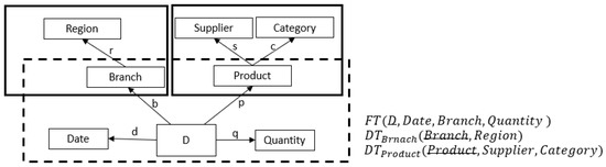
Figure 5.
A context and its underlying data stored in the form of a relation schema.
Our implementation handles the above relation schema as follows: The fact table is represented as an unbounded table containing the primary incoming streaming data, and the dimensional tables and are represented as static tables which are connected to the fact table. By using static dimensional tables, we avoid the stream-stream joins. The problem of generating inner join results between the two data streams is that, at any time, the view of the dataset is incomplete for both sides of the joining, making it inefficient to find the matching values between two inputs data streams. Any row received from the input stream can match with any future not yet received row from the other input stream. Thus, the solution for this is to buffer the past input as a streaming state to match every future input with past input and accordingly to generate join results. As such, our implementation supports joins between a streaming and static relational table.
In this setting, consider the query in the context of Figure 5, asking for totals by branch. In this query, the grouping and measuring attributes appear in the same fact table. This query will be mapped to the following SQL query:
- Select Branch, sum(Quantity) As ansQ(Branch)
- From FT
- Group by Branch
Next we present another example. Consider again the context in Figure 5 and assume we need to evaluate the following query asking for the totals by supplier and category. In this query, the grouping attributes supplier and category appear different in the table from the measuring attribute quantity. We map Q to the following SQL query over a star schema:
- Select Supplier, Category, sum(Quantity)
- As ansQ(Supplier, Category)
- From join (FT, DTProduct)
- Group by Supplier, Category
In the Input Preparation step, the grouping attributes are selected, which are the grouping attributes supplier and category and the measuring attribute quantity. The attributes supplier and category appear in the dimensional table so the fact table and the dimensional table are joined accordingly. The Grouping Partition Construction is performed by the “group by” clause to group rows that have the same attributes supplier and category. In Grouping Partition Reduction, the query operation sum is applied to the measuring attribute quantity. The ‘’ is a user defined attribute and the query returns the answer of Q in the form of a table with two attributes, and .
Rewritings to SQL
In this section, we present a detailed description of how the evaluation mechanism leverages these rules and an HIFUN rewritten set Q mapped to a physical-level mechanism of Spark Structured Streaming, and the semantics of SQL when the evolving datasets are stored in an unbounded append-only relation table.
Common Grouping and Measuring Rewriting Rule. In this rewriting rule, the SQL query is created by customizing the reduction step of SQL group-by query by adding the aggregate functions related to the n operations on the common measuring attribute, which appears in the rewritten HIFUN Q set.
Common Grouping Rewriting Rule. In this rewriting, the SQL query is created similarly to the previous rewriting rule. In the reduction step of the SQL group-by query, the aggregate functions are added to the n operations for the n corresponding measuring attributes—which appear in the rewritten HIFUN Q set.
Common Measuring and Operation Rewriting Rule and Basic Rewriting Rule. These rewriting rules are not supported when Spark Structured Streaming is used as the physical-level evaluation engine. Firstly, the evaluation of the the base query produces the base table used to evaluate the next queries. Each one of the outer queries uses the base table to produce the final answer. The above computations are achievable under the SQL semantics by mapping the base HIFUN query to a SQL group-by query, and each one of the outer queries also to SQL group-by queries. In the current version of Spark Structured Streaming, multiple streaming aggregations (i.e., chain of aggregation on a streaming DataFrame) are not supported yet.
5. Results
In this section, we describe the experiments that we conducted to verify the effectiveness of the query rewriting rules implemented. The purpose is to verify the extent to which the proposed incremental query mechanism with and without the rewriting rules will result in a significant performance gain to the overall query evaluation. More specifically, in our experiments, first we compared our incremental approach with the batch processing approach to show the benefits that we can get for continuous queries when evaluated incrementally to avoiding unnecessary query evaluations. We also present further performance gains achieved through our proposed rewritings.
5.1. Setup and Datasets
For our experiments we used a cluster that consisted of four nodes, each equipped with 38 cores at 2.2 GHz, 250 GB RAM and 1 TB storage. A synthetic dataset, 50 GB, was split into 10 files of 5 GB each (80 million records). Our contribution in this paper lies mainly in the definition of the query rewriting rules for the HIFUN language and their implementations in two versatile low-level configurations that demonstrate the generality of the approach. As such, the experiments presented in this section only verify the applicability of the whole approach. The source code, the dataset and the queries can be found online (https://github.com/petrosze/ContHIFUN accessed on 8 May 2021).
Each dataset is represented as an RDD and each RDD was pushed into a queue and treated as a batch of data in the DStream, and processed like a stream. To distribute the data uniformly among all the cluster workers, the data follow a uniform distribution. The following experiments were conducted in synthetic datasets stored in distributed file system (HDFS). In the case of the MapReduce execution model, the source dataset was provided in a single text file, and the analysis context of this dataset is depicted in Figure 6, whereas in the case of the SQL execution model, the source dataset was structured according to relational table, and the analysis context of this dataset is depicted in Figure 7. The attribute values were produced following uniform distribution, achieving a workload balance between all cluster nodes used.
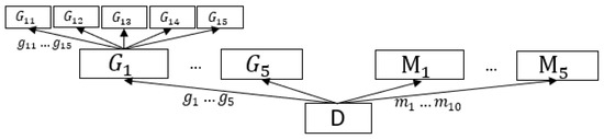
Figure 6.
Analysis context of the unstructured dataset.
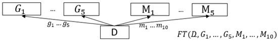
Figure 7.
Analysis context of the structured dataset.
5.2. Results
In order to evaluate the effectiveness of the incremental evaluation approach and the benefits of query rewriting, we next present the two main focuses of our experimental evaluation: incrementality and query rewriting.
5.2.1. Defining the Queries
Evaluation of CGMR Rule. In order to evaluate the Common Grouping and Measuring Rewriting Rule, the grouping attribute and the measuring attribute, was used to create a set Q of five queries with five different aggregation operations applicable to measuring attribute . The query set Q is defined as follows:
The equivalent rewritten of Q by this rule is the following query:
Evaluation of the CGR Rule. In order to evaluate the Common Grouping Rewriting Rule, the grouping attribute and five measuring attributes, are used to create a set Q of five queries with five different aggregation operations applicable to those measuring attributes. The query set Q is defined as follows:
The equivalent rewritten of Q by this rule is the following query:
Evaluation of the CMOR Rule. In order to evaluate the Common Measuring and Operation Rewriting Rule, the attributes … are used as grouping attributes, the attribute is used as a measuring attribute and the aggregation operation is a sum applied to measuring attribute .
The equivalent rewritten of Q by this rule is the following query:
Evaluation of the BR Rule. We define the following set of queries:
Q contains five queries, and all of them have the same distributive operation applicable to the same measuring attribute . As described by the rewriting theory, Q can be equivalently rewritten by the basic rewriting rule as follows:
5.2.2. Evaluating Incrementality
We evaluated the effectiveness of the incremental approach, contrasting it to the batch approach. The batch computation approach looks at the entire dataset when new data are available to be processed. From this perspective, two different scenarios were evaluated: In the first scenario, Q was executed by the evaluation of the included queries individually (e.g., without rewriting), and in the second scenario, the rewritten set was executed as defined by the rewritten theory. The incremental computation approach is more efficient by examining only the new incoming data in the last time interval and incorporates the increment in the result. From this perspective we evaluate the two scenarios again: the first scenario required the execution of the Q; the second scenario required the execution of rewritten .
Figure 8 and Figure 9 illustrate the evaluation times when Q and were executed using the MapReduce execution model and the two different approaches; Figure 10 illustrates the evaluation time when Q and are executed using the SQL execution model and the two different approaches. For example, at time , the batch computation approach requires one to execute the query set Q or the rewritten set , over all data generated in range of . At time , the incremental computation approach requires one to execute the query set Q or the rewritten set only on data generated in range of , and then incorporates the increment into the aggregated result.
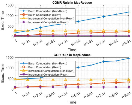
Figure 8.
Evaluation of CGMRR and CGRR when the MapReduce execution model is used over an unstructured dataset.
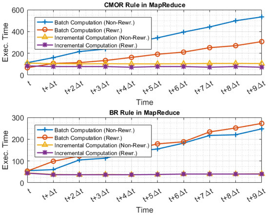
Figure 9.
Evaluation of CMORR and BRR when the MapReduce execution model is used over an unstructured dataset.
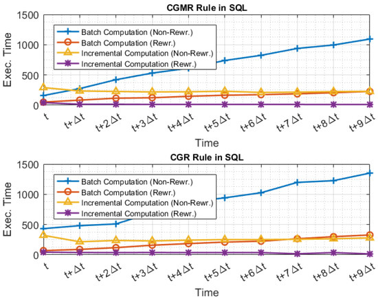
Figure 10.
Evaluation of CGMRR and CGRR when the SQL execution model is used over an structured dataset.
The experimental results presented in the figures demonstrate the effectiveness of our incremental computation. As shown, as the dataset grows, the evaluation cost remains stable independently of the overall increasing data size. On the other hand, when the queries are evaluated over a batch data, the evaluation cost grows linearly to the size of the input batch data. Furthermore, as shown, the execution time of the non-rewritten queries is dramatically higher as the dataset increases, independently of the applicable rewriting rule. However, when the rewritings are used, in total, querying consumes significantly less execution time, exploiting the shared common attributes. In addition, we can observe that the execution times are similar to when the MapReduce and the SQL execution models are used for the same rewritings (Figure 8 and Figure 10).
5.2.3. Evaluating Rewritings
In this experimental protocol we focused more on the effectiveness of the rewritings, when the incremental processing approach was used to refresh previously generated results. We also used the queries defined in previous experiment for each rewriting rule. Firstly, we evaluated the non-rewritten set Q by running the query evaluation process for it. We started by including only one query in Q, and gradually increasing the query number to reach queries. In this scenario, each included query in Q was executed for each micro-batch individually, and we report the average execution time. Secondly, we evaluated the execution of the rewritten set by starting again with one query () and gradually increasing the query number to . In this scenario, each included query in is executed for each micro-batch, and the average execution time is reported.
Figure 11 and Figure 12 illustrate the results for this series of experiments. As shown, when Q was executed without rewritting, the execution cost increased as the number of participating queries increased as well. Moreover, we observed that even with the more queries participating in the rewritten set , the execution cost remained the same. The variation in the execution time between the rewriting rules arose due to the nature of the queries included in the non-rewritten set Q and depends on the types of shared common attributes.
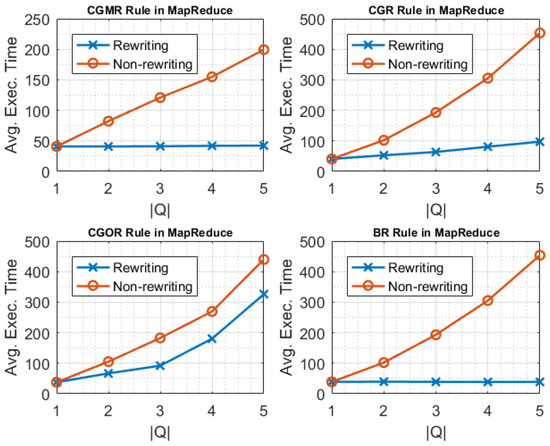
Figure 11.
Evaluation of rewriting rules for unstructured datasets, while the number of queries in the rewritten and non-rewritten set Q increases.
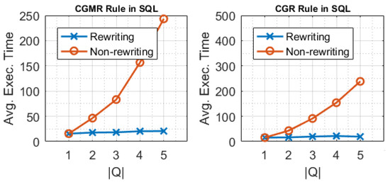
Figure 12.
Evaluation of CGMRR and CGRR for structured datasets, while the number of queries in the rewritten and the non-rewritten set Q increases.
The evaluation of and demonstrates that the reduction of evaluation cost was significant while the number of queries included in the query set increased. This is because the grouping construction and grouping reduction steps were performed once by applying the n operations, whereas in the case of the non-rewritten set, the grouping construction and grouping reduction steps were executed as many times as the number of queries included. The effectiveness of the and the rewritings was significant, as the number of included queries increased. The rewritten set consisted of five queries and each one used the answer of the base query as its measure. To investigate the effectiveness of the rewriting rule, we ran the experiments for the sets Q and , starting initially with one query and adding each time another one, till we reached a total number of five queries to be executed each time. We noticed that as more queries participated in the rewritten , a significant improvement in the performance resulted due the exploitation of the intermediate answers of each additional query.
6. Conclusions
In this paper, we leveraged the HIFUN language, while adding an incremental evaluation mechanism using Spark Streaming. We presented an approach allowing the incremental updating of continuous query results, thereby preventing costly re-computation from scratch. We also showed the additional benefits of query rewriting, enabled by the adoption of the HIFUN language. The query rewriting rules can be implemented in the physical layer as well, further benefiting the efficiency of query answering. We demonstrated experimentally the considerable advantages gained by using the incremental evaluation—reducing the overall evaluation cost using both the MapReduce implementation and the SQL one. Our system provides a compact solution for big data analytics and can be extended to support a big variety of dataset formats; its evaluation mechanisms work regardless of the nature of the data.
Limitations and Future Work
As a next step we intend to extend our system to make it capable of low-latency query processing. A critical aspect in real life applications is the evaluation of a query in the millisecond low-latency processing mode of streaming called continuous mode. Our implementation exploits stream processing capabilities through micro-batching. The main disadvantage of this approach is that each query is evaluated on a micro-batch, which needs to be collected and scheduled at regular intervals. This introduces latency. However, in real world use cases, we want to analyze and detect interesting patterns almost instantly. The continuous processing mode which we intend to explore next attempts to overcome this limitation by avoiding launches of periodic tasks and processes the incoming data in real-time. However, applying our model to that setting is challenging and will require further research. Finally, another limitation of our paper is the fact that real world data in many cases have missing values and nulls which should be appropriately tackled, whereas data distribution also plays an essential role in query efficiency. However, those topics are orthogonal to our approach and fall outside the scope of our paper.
Author Contributions
Formal analysis, P.Z.; methodology, H.K. and N.S.; software, P.Z.; supervision, N.S. and D.P.; writing—original draft, P.Z.; writing— review and editing, N.S. and D.P. All authors have read and agreed to the published version of the manuscript.
Funding
This research received no external funding.
Conflicts of Interest
The authors declare no conflict of interest.
References
- Mello, B.; Rios, R.; Lira, C.; Prazeres, C. FoT-Stream: A Fog platform for data stream analytics in IoT. Comput. Commun. 2020, 164, 77–87. [Google Scholar] [CrossRef]
- Kondylakis, H.; Dayan, N.; Zoumpatianos, K.; Palpanas, T. Coconut: Sortable summarizations for scalable indexes over static and streaming data series. VLDB J. 2019, 28, 847–869. [Google Scholar] [CrossRef]
- Queiroz, W.; Capretz, M.A.; Dantas, M. An approach for SDN traffic monitoring based on big data techniques. J. Netw. Comput. Appl. 2019, 131, 28–39. [Google Scholar] [CrossRef]
- Carcillo, F.; Dal Pozzolo, A.; Le Borgne, Y.A.; Caelen, O.; Mazzer, Y.; Bontempi, G. SCARFF: A scalable framework for streaming credit card fraud detection with spark. Inf. Fusion 2018, 41, 182–194. [Google Scholar] [CrossRef]
- Banerjee, A.; Chakraborty, C.; Kumar, A.; Biswas, D. Chapter 5—Emerging trends in IoT and big data analytics for biomedical and health care technologies. In Handbook of Data Science Approaches for Biomedical Engineering; Balas, V.E., Solanki, V.K., Kumar, R., Khari, M., Eds.; Academic Press: Cambridge, MA, USA, 2020; pp. 121–152. [Google Scholar] [CrossRef]
- Kondylakis, H.; Bucur, A.I.D.; Crico, C.; Dong, F.; Graf, N.M.; Hoffman, S.; Koumakis, L.; Manenti, A.; Marias, K.; Mazzocco, K.; et al. Patient empowerment for cancer patients through a novel ICT infrastructure. J. Biomed. Inform. 2020, 101, 103342. [Google Scholar] [CrossRef]
- Agathangelos, G.; Troullinou, G.; Kondylakis, H.; Stefanidis, K.; Plexousakis, D. Incremental Data Partitioning of RDF Data in SPARK; Springer: Cham, Swizterland, 2018. [Google Scholar]
- Kondylakis, H.; Plexousakis, D. Ontology Evolution in Data Integration: Query Rewriting to the Rescue. In Proceedings of the Conceptual Modeling—ER 2011, 30th International Conference, ER 2011, Brussels, Belgium, 31 October–3 November 2011; Volume 6998, Lecture Notes in Computer Science. Jeusfeld, M.A., Delcambre, L.M.L., Ling, T.W., Eds.; Springer: Berlin/Heidelberg, Germany, 2011; pp. 393–401. [Google Scholar] [CrossRef]
- Pappas, A.; Troullinou, G.; Roussakis, G.; Kondylakis, H.; Plexousakis, D. Exploring Importance Measures for Summarizing RDF/S KBs. In Proceedings of the Semantic Web—14th International Conference—ESWC 2017, Portorož, Slovenia, 28 May–1 June 2017; Part I; Volume 10249, Lecture Notes in Computer Science. pp. 387–403. [Google Scholar] [CrossRef]
- Troullinou, G.; Kondylakis, H.; Stefanidis, K.; Plexousakis, D. Exploring RDFS KBs Using Summaries. In Proceedings of the Semantic Web—ISWC 2018—17th International Semantic Web Conference, Monterey, CA, USA, 8–12 October 2018; Part I; Lecture Notes in Computer Science. Springer: Berlin/Heidelberg, Germany, 2018; Volume 11136, pp. 268–284. [Google Scholar] [CrossRef]
- Bolt, C.R. Hadoop: The Definitive Guide; OReilly Media, Inc.: Sebastopol, CA, USA, 2014. [Google Scholar]
- Dean, J.; Ghemawat, S. MapReduce: Simplified data processing on large clusters. Commun. ACM 2008, 51, 107–113. [Google Scholar] [CrossRef]
- Jakóbczyk, M.T. Practical Oracle Cloud Infrastructure; Springer: Berlin/Heidelberg, Germany, 2020. [Google Scholar]
- Karimov, J.; Rabl, T.; Katsifodimos, A.; Samarev, R.; Heiskanen, H.; Markl, V. Benchmarking Distributed Stream Data Processing Systems. In Proceedings of the 2018 IEEE 34th International Conference on Data Engineering (ICDE), Paris, France, 16–19 April 2018; pp. 1507–1518. [Google Scholar]
- Zaharia, M.; Das, T.; Li, H.; Hunter, T.; Shenker, S.; Stoica, I. Discretized streams: Fault-tolerant streaming computation at scale. In Proceedings of the Twenty-Fourth ACM Symposium on Operating Systems Principles, Farmington, PA, USA, 3–6 November 2013. [Google Scholar]
- Armbrust, M.; Das, T.; Torres, J.; Yavuz, B.; Zhu, S.; Xin, R.; Ghodsi, A.; Stoica, I.; Zaharia, M. Structured Streaming: A Declarative API for Real-Time Applications in Apache Spark. In Proceedings of the 2018 International Conference on Management of Data, Houston, TX, USA, 10–15 June 2018. [Google Scholar]
- Iqbal, M.; Soomro, T.R. Big Data Analysis: Apache Storm Perspective. Int. J. Comput. Trends Technol. 2015, 19, 9–14. [Google Scholar] [CrossRef]
- Carbone, P.; Katsifodimos, A.; Ewen, S.; Markl, V.; Haridi, S.; Tzoumas, K. Apache Flink™: Stream and Batch Processing in a Single Engine. IEEE Data Eng. Bull. 2015, 38, 28–38. [Google Scholar]
- Akidau, T.; Bradshaw, R.W.; Chambers, C.; Chernyak, S.; Fernández-Moctezuma, R.; Lax, R.; McVeety, S.; Mills, D.; Perry, F.; Schmidt, E.; et al. The Dataflow Model: A Practical Approach to Balancing Correctness, Latency, and Cost in Massive-Scale, Unbounded, Out-of-Order Data Processing. Proc. VLDB Endow. 2015, 8, 1792–1803. [Google Scholar] [CrossRef]
- Alami, K.; Maabout, S. A framework for multidimensional skyline queries over streaming data. Data Knowl. Eng. 2020, 127, 101792. [Google Scholar] [CrossRef]
- Ramesh, S.; Baranawal, A.; Simmhan, Y. Granite: A distributed engine for scalable path queries over temporal property graphs. J. Parallel Distrib. Comput. 2021, 151. [Google Scholar] [CrossRef]
- Kvet, M.; Matiasko, K. Flower Master Index for Relational Database Selection and Joining; Springer: Cham, Switzerland, 2021; pp. 181–202. [Google Scholar] [CrossRef]
- Kvet, M.; Kršák, E.; Matiaško, K. Study on Effective Temporal Data Retrieval Leveraging Complex Indexed Architecture. Appl. Sci. 2021, 11, 916. [Google Scholar] [CrossRef]
- Dam, T.L.; Chester, S.; Nørvåg, K.; Duong, Q.H. Efficient top-k recently-frequent term querying over spatio-temporal textual streams. Inf. Syst. 2021, 97, 101687. [Google Scholar] [CrossRef]
- Dhont, M.; Tsiporkova, E.; Boeva, V. Layered Integration Approach for Multi-View Analysis of Temporal Data; Springer: Cham, Switzerland, 2020; pp. 138–154. [Google Scholar] [CrossRef]
- Babu, S.; Widom, J. Continuous queries over data streams. SIGMOD Rec. 2001, 30, 109–120. [Google Scholar] [CrossRef]
- Franklin, A.; Gantela, S.; Shifarraw, S.; Johnson, T.R.; Robinson, D.J.; King, B.R.; Mehta, A.M.; Maddow, C.L.; Hoot, N.R.; Nguyen, V.; et al. Dashboard visualizations: Supporting real-time throughput decision-making. J. Biomed. Inform. 2017, 71, 211–221. [Google Scholar] [CrossRef]
- Laurent, D.; Lechtenbörger, J.; Spyratos, N.; Vossen, G. Monotonic complements for independent data warehouses. VLDB J. 2001, 10, 295–315. [Google Scholar] [CrossRef][Green Version]
- Ahmad, Y.; Kennedy, O.; Koch, C.E.; Nikolic, M. DBToaster: Higher-order Delta Processing for Dynamic, Frequently Fresh Views. Proc. VLDB Endow. 2012, 5, 968–979. [Google Scholar] [CrossRef]
- Spyratos, N.; Sugibuchi, T. HIFUN—A high level functional query language for big data analytics. J. Intell. Inf. Syst. 2018, 51, 529–555. [Google Scholar] [CrossRef]
- Spyratos, N.; Sugibuchi, T. A High Level Query Language for Big Data Analytics. Available online: http://publications.ics.forth.gr/tech-reports/2017/2017.TR467_HiFu_Query_Language_Big_Data_Analytics.pdf (accessed on 8 May 2021).
- Papadaki, M.E.; Spyratos, N.; Tzitzikas, Y. Towards Interactive Analytics over RDF Graphs. Algorithms 2021, 14, 34. [Google Scholar] [CrossRef]
- Zervoudakis, P.; Kondylakis, H.; Plexousakis, D.; Spyratos, N. Incremental Evaluation of Continuous Analytic Queries in HIFUN. In International Workshop on Information Search, Integration, and Personalization; Springer: Cham, Switzerland, 2019; pp. 53–67. [Google Scholar]
- Garcia-Molina, H.; Ullman, J.D.; Widom, J. Database Systems—The Complete Book (International Edition); Pearson Education: London, UK, 2002. [Google Scholar]
- Le, D.; Chen, R.; Bhatotia, P.; Fetze, C.; Hilt, V.; Strufe, T. Approximate Stream Analytics in Apache Flink and Apache Spark Streaming. arXiv 2017, arXiv:1709.02946. [Google Scholar]
- Terry, D.; Goldberg, D.; Nichols, D.; Oki, B.M. Continuous queries over append-only databases. In Proceedings of the SIGMOD ’92, San Diego, CA, USA, 3–5 June 1992. [Google Scholar]
- Chen, J.; DeWitt, D.; Tian, F.; Wang, Y. NiagaraCQ: A scalable continuous query system for Internet databases. In Proceedings of the SIGMOD ’00, Dallas, TX, USA, 16–18 May 2000. [Google Scholar]
- Liu, L.; Pu, C.; Tang, W. Continual Queries for Internet Scale Event-Driven Information Delivery. IEEE Trans. Knowl. Data Eng. 1999, 11, 610–628. [Google Scholar]
Publisher’s Note: MDPI stays neutral with regard to jurisdictional claims in published maps and institutional affiliations. |
© 2021 by the authors. Licensee MDPI, Basel, Switzerland. This article is an open access article distributed under the terms and conditions of the Creative Commons Attribution (CC BY) license (https://creativecommons.org/licenses/by/4.0/).