Article

An Improved Artificial Bee Colony for Feature Selection in QSAR

College of Computer and Information Sciences, Fujian Agriculture and Forestry University, Fuzhou 350002, China
*
Author to whom correspondence should be addressed.
These authors contributed equally to this work.
Algorithms 2021, 14(4), 120; https://doi.org/10.3390/a14040120
Submission received: 9 March 2021 / Revised: 2 April 2021 / Accepted: 7 April 2021 / Published: 9 April 2021

Abstract

:
Quantitative Structure–Activity Relationship (QSAR) aims to correlate molecular structure properties with corresponding bioactivity. Chance correlations and multicollinearity are two major problems often encountered when generating QSAR models. Feature selection can significantly improve the accuracy and interpretability of QSAR by removing redundant or irrelevant molecular descriptors. An artificial bee colony algorithm (ABC) that mimics the foraging behaviors of honey bee colony was originally proposed for continuous optimization problems. It has been applied to feature selection for classification but seldom for regression analysis and prediction. In this paper, a binary ABC algorithm is used to select features (molecular descriptors) in QSAR. Furthermore, we propose an improved ABC-based algorithm for feature selection in QSAR, namely ABC-PLS-1. Crossover and mutation operators are introduced to employed bee and onlooker bee phase to modify several dimensions of each solution, which not only saves the process of converting continuous values into discrete values, but also reduces the computational resources. In addition, a novel greedy selection strategy which selects the feature subsets with higher accuracy and fewer features helps the algorithm to converge fast. Three QSAR datasets are used for the evaluation of the proposed algorithm. Experimental results show that ABC-PLS-1 outperforms PSO-PLS, WS-PSO-PLS, and BFDE-PLS in accuracy, root mean square error, and the number of selected features. Moreover, we also study whether to implement scout bee phase when tracking regression problems and drawing such an interesting conclusion that the scout bee phase is redundant when dealing with the feature selection in low-dimensional and medium-dimensional regression problems.

1. Introduction

Quantitative structure–activity relationship (QSAR) plays a vital role in drug design and discovery [1]. It aims to build the relationship between molecular structure properties of chemical compounds and their corresponding biological activities [2]. In QSAR modeling, the structure properties of the chemical compounds are encoded by a variety of features (molecular descriptors) such as topological, constitutional, thermodynamic parameters. QSAR models can be defined as regression or classification models by using different computational strategies [3]. The features are related with biological activities by using statistical methods or artificial intelligence approaches, such as Multiple Linear Regression (MLR) [4], Support Vector Regression (SVR) [5], Boosted Tree [6], and Partial Least Squares (PLS) regression [7], etc. In particular, machine learning methods have become extensively used in this field during the last few years [8,9,10,11,12,13,14,15]. These methods effectively improve the accuracy of QSAR modeling to a certain extent.
However, several computational issues must be addressed when QSAR models are inferred by machine learning methods. One of these problems is to address the complexity of data sets for selection of appropriate features important for defining a particular QSAR model. Specifically, not all features are related to the activity, and the redundant or irrelevant features may cause over-fitting or weak correlation [16]. The optimal feature subset with only related and non-redundant features increases the accuracy of prediction and the interpretability of the QSAR model. Thus, feature selection (FS) which selects an optimal subset of all features is a vital pre-processing step in QSAR studies to increase the interpretability and improve the prediction accuracy [17].
In principle, feature selection is an NP-hard combination problem. For a search space with D dimensions, the number of subsets to search is 2 D . In other words, the search space increases exponentially as the dimension of the given problem grows, hence it is intractable for limited computational resources.
Evolutionary Computation (EC) techniques are optimization methods inspired by scientific understanding of natural or social behavior, which can be regarded as search procedures at some abstraction level [18]. In general, these algorithms can be classified as either Evolutionary Algorithms (EAs) or Swarm Intelligence (SI) algorithms [19]. EAs start by randomly generating a set of candidate solutions, iteratively combine these solutions, and implement survival of the fittest until an acceptable solution is achieved. The classic EAs include Genetic Algorithm (GA) [20], Differential Evolution (DE) [21], Biogeography-Based Optimization (BBO) [22], and Genetic Programming (GP) [23], etc. SI algorithms start with a set of individuals, and a new set of individuals is created based on historical information and related information in each iteration. A considerable number of new SI algorithms have emerged, such as Ant Colony Algorithm (ACO) [24], Bat Algorithm (BA) [25], Firefly Algorithm (FA) [26], Cuckoo Search (CS) [27], Coyote Optimization Algorithm (COA) [28], and Social Network Optimization (SNO) [29].
SI is a relatively new category of evolutionary computation comparing with EAs and other single-solution based approaches and has paid sufficient attention to feature selection due to its potential global search ability. In particular, the interaction between features can be considered in the screening process, which breaks through the shortcomings of traditional feature selection algorithms. The surveys [30,31] have presented the proven usage of SI algorithms for FS.
The Artificial Bee Colony (ABC) [32] algorithm, which simulates the intelligent foraging behavior of a honeybee swarm, is one of the most well-known SI algorithms. Karaboga et al. concluded that, although ABC uses fewer control parameters, it performs better than or at least comparable to other typical SI algorithms [33]. Ozger et al. [34] carried out a comparative study on different binary ABC algorithms on feature selection. BitABC [35] employs bitwise operators such as AND, OR, XOR to generate new candidate solutions, and the binary ABC algorithm uses different functions to convert continuous vector to binary vectors, such as rounding function [36], sigmoid function [37], and tangent function [38]. The experimental results showed that BitABC generated better feature subsets in shorter computational time. Moreover, many studies combine ABC with other optimization algorithms, such as DE [39], ACO [40], and PSO [41], and they achieve promising results as well. However, the ABC algorithm is seldom applied to regression and prediction problems and achieve promising results.
To improve the accuracy and interpretability of QSAR that is a regression and prediction problem, we apply ABC algorithm to feature selection in QSAR. Major novelties and contributions of our study are described as follows:
(1)
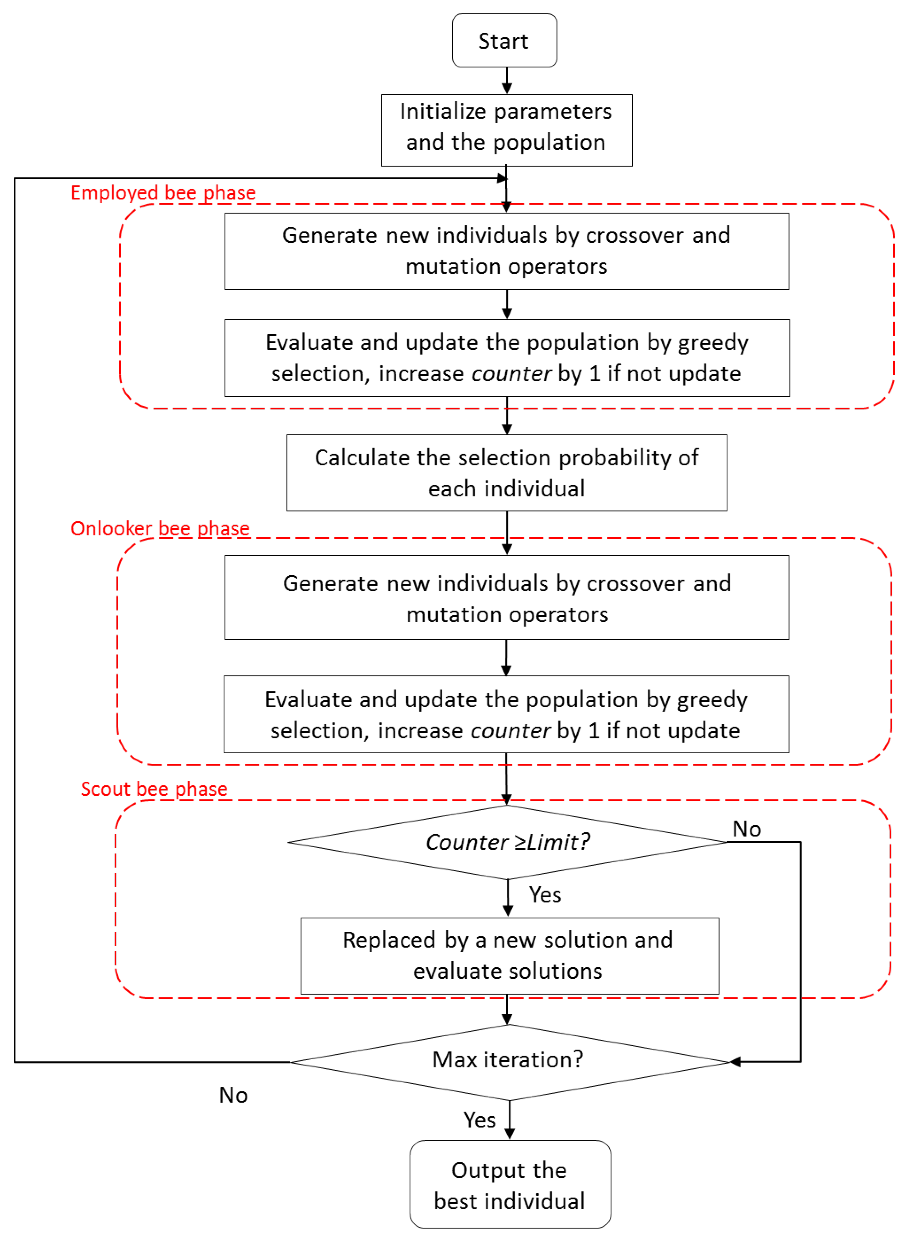
To save the process of converting continuous space into discrete space and reduce the consumption of computing resources, a two-point crossover operator and a two-way mutation operator are employed to generate food sources in employed bee phase and onlooker bee phase.
(2)
To achieve fast convergence, a novel greedy selection strategy is employed to greatly reduce the possibility of food sources being abandoned.
(3)
Furthermore, we investigate the influence of different threshold values that determine whether to implement the scout bee phase on the performance of QSAR and draw an interesting conclusion that the scout bee phase is redundant when dealing with the feature selection in low-dimensional and medium-dimensional regression problem.
The rest of this paper is organized as follows: Section 2 reviews the related work of FS methods based on SI. Section 3 briefly describes QSAR modeling and the FS problem. Section 4 presents the basic ABC algorithm and proposes two improved ABC variants for FS in QSAR. Section 5 describes the experimental datasets and parameter settings. Section 6 presents the experimental results. Conclusions are given in Section 7.

2. Related Work

SI algorithms are well-known for their global exploration capability and are gaining more attention by the feature selection community recently. It has been proven by the well-known “No Free Lunch (NFL) theorem” [42] that there is no heuristic algorithm that can solve all types of optimization problems. Specifically, since the exploration—exploitation balance is an unsolved issue within SI algorithms, each SI algorithm introduces an experimental solution through the combination of deterministic models and stochastic principles. Under such conditions, each SI algorithm holds distinctive characteristics that properly satisfy the requirements of particular problems [18]. Therefore, a particular SI algorithm is not able to solve all problems adequately. This motivates many researchers to investigate the effectiveness of different algorithms in different fields. Between 2010 and 2020, there have been a total of 85 papers used SI algorithms for feature selection in different fields [30].
For the medical application, Mehrdad et al. integrated the node centrality and PSO algorithm [43] to improve the performance on FS. Neggaz et al. [44] applied the sine–cosine algorithm and the disruption operator to Salp Swarm Algorithm (SSA) to improve the accuracy of disease diagnosis. Mafarja and Mirjalili [45] proposed a novel Whale Optimization Algorithm (WOA) for FS, and the crossover and mutation operators are used to enhance the exploitation of the WOA algorithm. An FS method suppressed less relevant features in the breast cancer datasets by ABC. Then, to minimize the potential of ABC being trapped in a local optimum, the accuracy of classification by GBDT is employed to evaluate the quality of the inputs [46]. To select a DNA microarray subset of relevant and non-redundant features for computational complexity reduction, Indu et al. [47] proposed a two-phase hybrid model based on improved-binary PSO (iBPSO). A recursive PSO method was developed by Prasad et al. [48] for gene selection. Ahead of this, an Ant Colony Optimization-selection (ACO-S) is utilized to generate a gene subset with the smallest size and salient features while yielding high classification accuracy [49]. Furthermore, Yan et al. [50] hybridized the V-WSP, proposed by Ballabio et al. [51], with PSO to improve the accuracy of laser-induced breakdown spectroscopy. Moreover, to solve the feature selection problem for acoustic defect detection, a single-objective feature selection algorithm hybridizing the Shuffled Frog Leaping Algorithm (SFLA) with an improved minimum-redundancy maximum-relevancy (ImRMR) was proposed by Zhang et al. [52]. To handle the challenges of the network detection that detecting anomalies from high dimensional network traffic feature is time-consuming, an FA-based feature selection was attempted by Selvakumar and Muneeswaran [53]. to obtain an optimized detection rate. In addition, FS methods based on the firefly algorithm were investigated for Arabic text classification. Ref. [54] and facial expression classification [55].
Additionally, various SI algorithms have been applied to FS in QSAR. Kumar et al. [56] first used multi-layer variable selection strategy, and then used GA to select meaningful descriptors from a large set of initial descriptors. PSO has been widely applied to selection descriptors in QSAR. For instance, Shen et al. [57] modified PSO named PSO-PLS for variable selection in MLR and PLS modeling. The hybridization of PSO with GA are used as a FS technique by Goodarzi et al. [58]. After that, Wang et al. [59] proposed a weighted sampling PSO-PLS (WS-PSO-PLS) to select the optimal descriptor subset in the QSAR/QSPR model. Moreover, the improved binary Pigeon Optimization Algorithm (POA) was applied to selecting the most relevant descriptors (variables) in QSAR/QSPR classification models [60].
Compared with PSO and ACO, there are fewer studies applying ABC algorithm to FS. Most of them are applied to classification or clustering problems, and rarely used to select features for regression problems. Therefore, in this paper, the ABC algorithm is used to select features for PLS modeling, which is the most straightforward linear regression-based modeling method in QSAR.

3. Preliminaries

3.1. QSAR Modeling

In QSAR study, the number of parameters describing the molecular structure of compounds is generally much larger than the number of samples, and there may be obvious chance correlations and multicollinearity between these parameters. By decomposing and screening the information in the data system, the Partial Least Squares (PLS) method can extract the variables with a strong explanation to overcome the adverse effects of chance correlations and multicollinearity in modeling. Therefore, the PLS method is often used as a prediction model for QSAR modeling.
The PLS method is often utilized to predict the relationship between compounds and their corresponding biological activities or chemical properties. It models the relationship between two data matrices, the independent variables X and target variable Y, by a linear multivariate model with factor analysis [61]. The basic principle of PLS regression depends on latent variables. Latent variables are extracted from a set of descriptors that include the basic information essential for modeling the target. QSAR is modeled by using a dependent (response variable) and several independent (molecular descriptors) variables.
The value of Q 2 , a well-known metric which employs the cross-validation technique, measures the accuracy of QSAR modeling, and it is defined as follows:
Q 2 = 1 i = 1 n ( y i y i ^ ) i = 1 n ( y i y i ¯ )
where y i , y i ^ , and y i ¯ are the observed value of activity of the compound, the predicted value by the PLS model via using cross-validation procedure, and the average observed value of all compounds, respectively. n is the total number of compounds.

3.2. Feature Selection

Let S be a dataset of L samples with D features. A feature selection problem can be described as follows: selecting d features ( d < D ) from all features, to optimize a given function H ( · ) . In regression analysis and prediction, H ( · ) generally represents the accuracy or error rate. Generally, we use a binary string to encode a solution X in FS problems:
X = ( x 1 , x 2 , , x D ) , x j 0 , 1
where x j = 1 represents that the jth feature is selected into the subset X, otherwise, not selected. Then, taking the case of that function H ( · ) being prediction accuracy, the FS problem can be formulated as follows:
m a x H ( X ) s . t . X = ( x 1 , x 2 , , x D )

4. The Proposed Method

4.1. The Basic Artificial Bee Colony Algorithm

ABC is a swarm intelligence algorithm that simulates the foraging behavior of a honey bee colony [32]. It has been used widely in many fields for solving optimization problems [62]. In the hive, three types of bees are assigned to the foraging task: employed bees, onlooker bees, and scout bees. Employed bees use the previous source information to find better food sources and share the information with onlooker bees. Onlooker bees waiting on the hive exploit a source with the help of the information shared by employed bees. Scout bees search for undiscovered sources based on an internal rule or possible external clues. The basic implementation of ABC is as follows:
(1) Initialization phase: From the perspective of an optimization problem, each food source represents a probable solution which is described as a vector: X = ( x i , 1 , x i , 2 , , x i , D ) , and is generated by Equation (4):
x i , j = x j m i n + r a n d ( 0 , 1 ) ( x j m a x x j m i n )
where i = 1 , 2 , , S N and S N is the number of the food source. j = 1 , 2 , , D and D is the dimensionality of the search space. x i , j is the jth dimension of x i . x j m a x and x j m i n are the maximum and minimum boundary value, respectively.
(2) Employed bee phase: Each employed bee is associated with a food source. Employed bees need to modify the position of their food source to find new better ones. Thereby, they learn from a neighbor source which is selected randomly among all sources except for itself. The new food source is produced by Equation (5):
x i , j = x i , j + ϕ i , j ( x i , j x k , j )
In the above formula, ϕ i , j is a uniformly distributed random value within [−1,1]. After x i is produced, its fitness value can be evaluated according to Equation (1). Then, a greedy selection is applied to the selection between x i and x i . Specifically, if f ( x i ) > f ( x i ) , x i replaces x i to enter the next iteration and its counter holding, the number of trials is reset to 0. Otherwise, x i is kept into the next iteration and its counter holding the number of trials is increased by 1.
(3) Onlooker bee phase: After getting the information concerning nectar amount (fitness value) and positions of food sources from employed bees, each onlooker bee selects a food source according to the fitness values by a roulette-wheel scheme, where the better the fitness value of the source, the higher the probability of being selected. The probability value of each food source is calculated by Equation (6):
P i = f i t n e s s i j = 1 S N f i t n e s s j
After calculating the probability value of each source, a random number r a n d ( 0 , 1 ) is generated to determine whether to be chosen. If P i > r a n d ( 0 , 1 ) , x i is chosen to update just as in the employed bee phase.
(4) Scout bee phase: Each source has a counter which is zero at the beginning. If the counter holding the number of trials exceeds the predefined threshold value, its corresponding food source will be abandoned and replaced by a new food source, which is generated by Equation (4).

4.2. ABC Algorithm for FS in QSAR

The basic ABC algorithm is originally proposed for optimization problems in continuous space; however, FS is an optimization problem in discrete space. Each feature subset is represented with a binary string. “1” in the string means the feature is selected and “0” means the feature is not selected. Hence, the value obtained by Equation (4) needs to be converted into a discrete value by Equation (7):
x i , j = 1 , x i , j 0.5 0 , o t h e r w i s e
If the value of a dimension is greater than or equal to the threshold value 0.5, the corresponding feature is selected and then its value will be set as 1. Otherwise, it is not selected and its value will be set as 0. Accordingly, an ABC-based algorithm for feature selection in QSAR is proposed, namely ABC-PLS. The pseudo code of the ABC-PLS algorithm can be seen in Algorithm 1.
Algorithm 1 Pseudo code of the ABC-PLS algorithm
Input: Population size S N , Maximum number of iterations M a x I t , Abandonment limit L, c o u n t e r = 0 , t = 0 .
Output: The optimal food source x b e s t , the best fitness value f ( x b e s t ) .
1:
Initialize the population x i , ( i = 1 , 2 , S N ) by using Equation (4).
2:
Evaluate the fitness value of each food source by using Equation (1).
3:
while t M a x I t do
4:
    %Employed bee phase
5:
    for each employed bee do
6:
        Randomly select a different food source x k .
7:
        Generate a new food source according to Equation (5) and convert it into discrete values by using Equation (7).
8:
        Evaluate the fitness value of each food source by using Equation (1).
9:
        Update x i according to greedy selection, and increase its c o u n t e r counter by 1 if not update.
10:
    end for
11:
    Calculate the selection probability of each food source by using Equation (6).
12:
    %Onlooker bee phase
13:
    for each onlooker bee do
14:
        Select a food source x i according to the selection probability by the roulette-wheel scheme.
15:
        Randomly select a different food source x k .
16:
        Generate a new food source according to Equation (5) and convert it into discrete values by using Equation (7).
17:
        Evaluate the fitness value of each food source by using Equation (1).
18:
        Update x i according to greedy selection, and increase its c o u n t e r counter by 1 if not update.
19:
    end for
20:
    %Scout bee phase
21:
    for each food source do
22:
        if c o u n t e r L then
23:
           Replaced by a new food source according to Equation (5) and convert it into discrete values by Equation (7).
24:
           Evaluate the fitness value of the new food source by using Equation (1).
25:
        end if
26:
    end for
27:
end while
28:
Output x b e s t and f ( x b e s t ) .

4.3. An Improved ABC Algorithm for FS in QSAR

Since ABC-PLS needs to convert continuous values into discrete values in all four phases of the algorithm, it consumes more computational resources (time, memory). Inspired from Hancer [63], the two-point crossover operator and two-way mutation operator are employed to generate food sources in the employed bee phase and onlooker bee phase. In the algorithm proposed by Hancer, x i and x k generate two new food sources by the crossover operation, and generate another two new food sources by the mutation operator. Therefore, the size of a set with S N solutions will expand to 5 × S N after cross-mutation. Furthermore, the 5 × S N solutions are ranked using non-dominated sorting, and S N number of solutions are selected to update the population through rank and crowding distance. Instead of expanding the size of the solutions set, which consumes much computational time and memory, the two-point crossover operator and the two-way mutation operator used in this paper are described as follows:

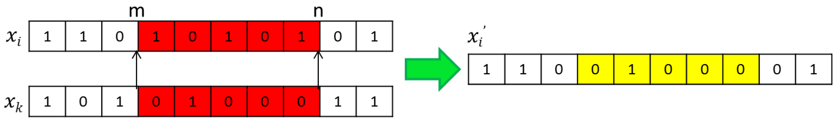
4.3.1. Two-Point Crossover

Crossover is operated between the current food source x i and a food source x k that is selected randomly ( x i x k ), two positions m and n are randomly determined on x i and x k ( m < n < D ). All values between the position of x i are copied to x i and generate a new food source [63]. An illustrative sample of crossover operator is presented in Figure 1.

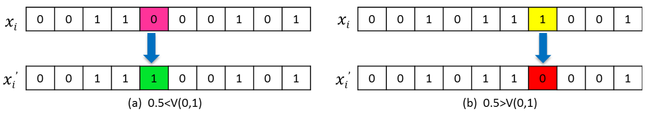
4.3.2. Two-Way Mutation Operator

First, a random number within the range of 0 and 1 is uniformly generated. If the generated number is greater than 0.5, a position with value 1 is randomly chosen and its position is set to 0. Otherwise, a position with value 0 is randomly chosen and its position is set to 1 [63]. In this way, a new food source is generated. The mutation operator used in this paper is shown as Figure 2.
Subsequently, in view of the fact that if the food source in the employed bee or onlooker bee phase is not updated for a long time, it will be abandoned and reinitialized to produce a new food source, which will reduce the convergence speed of the algorithm, a greedy selection strategy is employed after mutation, and it is specifically described as follows.

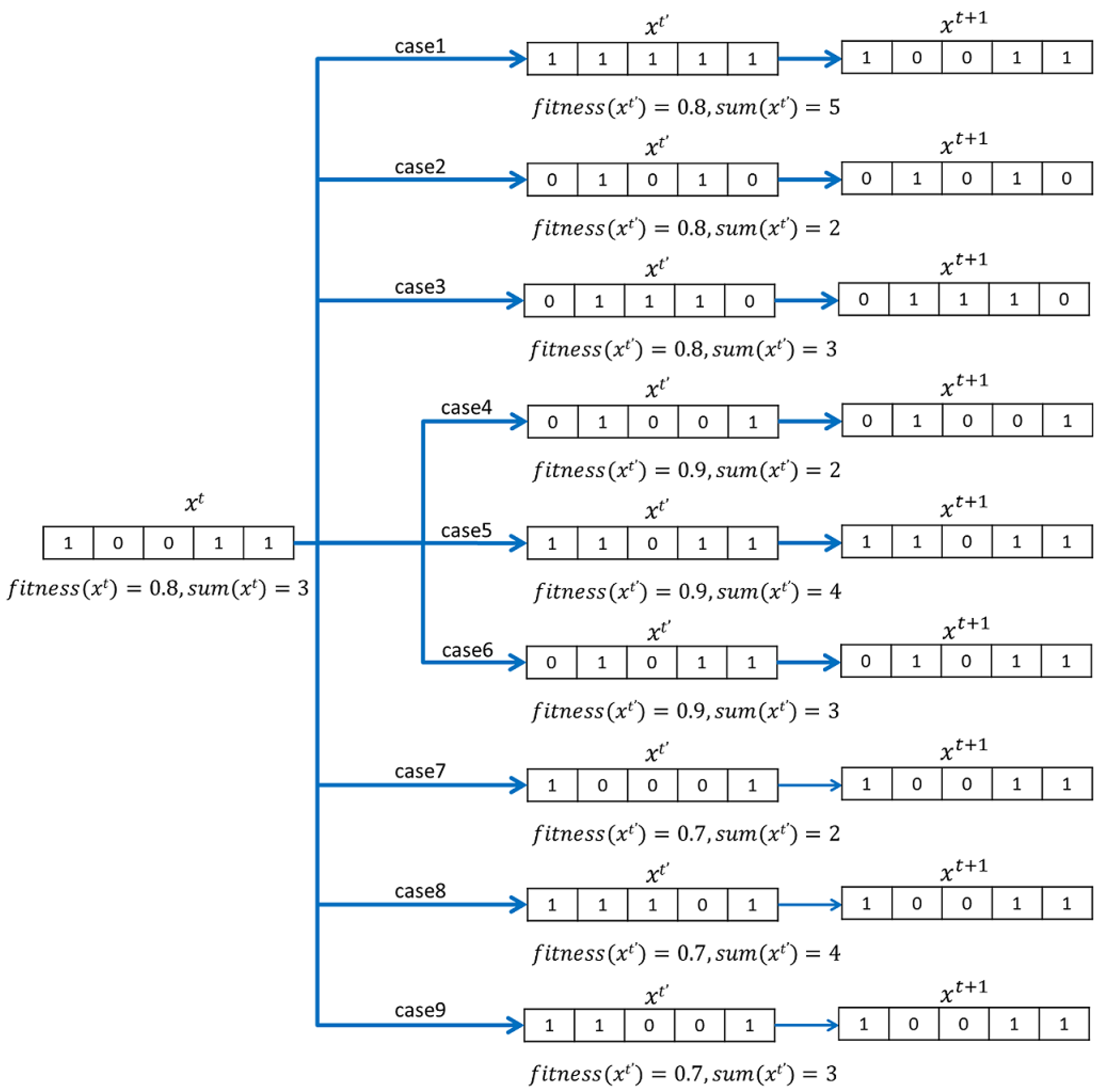
4.3.3. Novel Greedy Selection Strategy

If the fitness value of x i is higher than x i , x i replaces x i and enters next iteration. If the fitness of x i is the same as x i , but its number of selected features is less than or equal to the x i , x i replaces x i and enters next iteration as well. Else, x i enters the next iteration and x i is discarded. To make it easier to understand, we give the following example, as shown in Figure 3.
There are nine cases of whether an individual updates or not in Figure 3, where x t and x t denote food source and its offspring in the current iteration, respectively. x t + 1 denotes the individual entering the next iteration. f i t n e s s is the prediction accuracy and s u m is the number of selected features. The first three cases indicate that, if x t has the same fitness value with x t and its number of selected features is the same as or more than x t , it will be replaced by x t ; otherwise, it will enter the next iteration directly. If the fitness value of x t is smaller than x t , it will also be replaced by x t regardless of the number of features it selects, which is shown as cases 4–6. In another three cases, x t with a larger fitness value than x t will enter the next iteration without update.
Combining the above three together, the ABC-PLS-1 is proposed. Figure 4 shows the flowchart of ABC-PLS-1 and pseudo code is outlined in Algorithm 2. Overall, the two-point crossover and two-way mutation operators not only save on the process of converting continuous space into discrete space, but also reduce the consumption of computing resources. Furthermore, the greedy selection strategy greatly reduces the possibility of food sources being abandoned so that the algorithm can converge fast to the optimal solution, thereby, the scout bee phase of ABC algorithm does not improve the prediction performance, so it can be omitted. This conclusion will be verified by setting different thresholds that determine whether to carry out the scout bee phase.
Algorithm 2 Pseudo code of the ABC-PLS-1 algorithm
Input: Population size S N , Maximum number of iterations M a x I t , Abandonment limit L, c o u n t e r = 0 , t = 0 .
Output: The optimal food source x b e s t , the best fitness value f ( x b e s t ) .
1:
Initialize the population x i , ( i = 1 , 2 , S N ) by using Equation (4).
2:
Evaluate the fitness value of each food source by using Equation (1).
3:
while t M a x I t do
4:
    % Employed bee phase
5:
    for each employed bee do
6:
        Randomly select a different food source x k .
7:
        Generate a new food source by crossover operator and mutation operator on x i and x k .
8:
        Evaluate the fitness value of each food source by using Equation (1).
9:
        Update x i according to greedy selection, and increase its c o u n t e r counter by 1 if not update.
10:
    end for
11:
    Calculate the selection probability of each food source by using Equation (6).
12:
    % Onlooker bee phase
13:
    for each onlooker bee do
14:
        Select a food source x i according to the selection probability by roulette-wheel scheme.
15:
        Randomly select a different food source x k .
16:
        Generate a new food source by crossover operator and mutation operator on x i and x k .
17:
        Evaluate the fitness value of each food source by using Equation (1).
18:
        Update x i according to greedy selection, and increase its c o u n t e r counter by 1 if not update.
19:
    end for
20:
    %Scout bee phase
21:
    for each food source do
22:
        if c o u n t e r L then
23:
            Replaced by a new food source according to Equation (5) and convert it into discrete values by Equation (7).
24:
           Evaluate the fitness value of the new food source by using Equation (1).
25:
        end if
26:
    end for
27:
end while
28:
Output x b e s t and f ( x b e s t ) .

5. Experimental Design

5.1. Datasets and Parameters

To verify the performance of the proposed ABC-PLS and ABC-PLS-1 algorithm, a series of experiments are conducted on three common QSAR datasets: Artemisinin, benzodiazepine receptors(BZR), and Selwood. The Artemisinin dataset contains 178 compounds and 89 features. The BZR dataset contains 163 compounds and 75 features. The Selwood dataset contains 29 compounds and 53 features [59]. The basic information about the datasets is described in Table 1.
We investigate the performance of the proposed algorithms by comparing it with three FS algorithms for QSAR, including PSO-PLS [57], WS-PSO-PLS [59], and BFDE-PLS [64]. For the compared algorithms, the parameters are set as recommended in the corresponding papers. All algorithms are in MATLAB languages. The population size is 50, and the maximum number of iterations is 200. The thresholds value (i.e., L i m i t ) in the ABC algorithm is set to 100. For fair comparison, each algorithm runs 100 times independently. Table 2 gives the parameter settings of all algorithms.
All the algorithm operations are programmed by MATLAB (R2016b) produced by MathWorks, Natick, MA, USA. All experiments were run on an Intel Core i5 computer with a 3.40 GHz CPU and 8 GB RAM.

5.2. Performance Metric

A 5 fold cross-validation method is employed to evaluate the performance of QSAR. Here, the metric Q 2 reflects the prediction accuracy, and it is calculated as Equation (1). The number of features denotes N U M . To know more about the stability of the algorithm, the Root Mean Square Error ( R M S E ) is calculated as well, which is defined as follows:
R M S E = i = 1 n ( y i y i ^ ) 2 M X
where y i , y i ^ refer to the same as in Equation (1), and M X denotes the number of compounds.

6. Experimental Results and Analysis

Table 3 shows the experimental results of six QSAR methods.The best results are identified in boldface. Without introducing intelligent algorithms, the PLS model selects all features in each dataset, and the mean Q 2 and root mean square error are respectively 0.6 and 0.99 on the Artemisinin dataset, 0.4 and 0.85 on the BZR dataset, and 0.24 and 0.65 on the Selwood dataset. However, the performance of PLS is improved when the intelligent algorithm is introduced into the model. The experimental results show that the intelligent algorithm can eliminate the irrelevant features in the datasets by using global search or local search.
The following comparison results can be obtained from Table 3: on the Artemisinin dataset, the mean Q 2 of ABC-PLS-1 is 3.64% larger than that of PSO-PLS and 1.48% larger than that of WS-PSO-PLS, the root mean square error of ABC-PLS-1 is 5.73% smaller than that of PSO-PLS and 2.39% smaller than WS-PSO-PLS. On the BZR dataset, the mean Q 2 of ABC-PLS-1 is 1.8% larger than that of PSO-PLS and 1.29% larger than that of WS-PSO-PLS, the root mean square error of ABC-PLS-1 is 1.49% smaller than that of PSO-PLS and 1.07% smaller than that of WS-PSO-PLS, and the features selected by ABC-PLS-1 are 5.88 less than that selected by PSO-PLS and 4.14 less than that selected by WS-PSO-PLS. On the Selwood dataset, the mean Q 2 of ABC-PLS-1 is 6.73% larger than that of PSO-PLS and 1.74% larger than that of WS-PSO-PLS, the root mean square error of ABC-PLS-1 is 7.67% smaller than that of PSO-PLS and 2.28% smaller than that of WS-PSO-PLS, and the features selected by ABC-PLS-1 are 5.8 less than that selected by PSO-PLS and 3.16 less than that selected by WS-PSO-PLS. The mean Q 2 of ABC-PLS-1 is larger than that of BFDE-PLS and the root mean square error of ABC-PLS-1 is smaller than that of BFDE-PLS on all the three datasets. However, the features selected by ABC-PLS-1 is more than that selected by BFDE-PLS in the Artemisinin dataset and the BZR dataset. ABC-PLS-1 selects more features than ABC-PLS on the Artemisinin dataset, but it is superior to the ABC-PLS on the other two datasets.
In conclusion, although the number of selected features of ABC-PLS-1 is not smaller than that of BFDE-PLS on Artemisinin and BZR, the prediction accuracy and the root mean square error of ABC-PLS-1 is obviously better than ABC-PLS, PSO-PLS, WS-PSO-PLS, and BFDE-PLS on all the three datasets.
A rank sum test method at a significance level of 0.05 is used to compare mean Q 2 on three datasets to determine whether ABC-PLS-1 is significantly different from PSO-PLS, WS-PSO-PLS, BFDE-PLS, and ABC-PLS. As shown in Table 4, ABC-PLS-1 is significantly better than others in the mean Q 2 on all datasets.
Figure 5 shows the Q 2 obtained by each algorithm used by running 100 times on three datasets. It is obvious that the Q 2 of ABC-PLS-1 is generally higher than that of the other four algorithms on the Artemisinin dataset and the Selwood dataset. In the last subfigure, the Q 2 of ABC-PLS-1 is higher than PSO-PLS, WS-PSO-PLS, and ABC-PLS, and it is stable.
Convergence curves of the algorithms on three datasets are shown in Figure 6. Each curve is an average result of 100 runs in each iteration. ABC-PLS-1 converges faster with a good quality of solution compared to other state of-the-art methods on Artemisinin and BZR datasets. Although BFDE-PLS finally converges to a higher quality solution than ABC-PLS-1 on the Selwood dataset, it is greatly inferior to others on Artemisinin and BZR datasets and its convergence speed is slow. Overall, ABGWO achieved better performance than others with respect to both convergence speed and solution quality.
Furthermore, in order to verify the validity of ABC-PLS-1, the Root Mean Square Error (RMSE) of ABC-PLS-1 is compared with that of the other four algorithms. Figure 7 presents Box-plots which show the RMES of the five algorithms on three datasets. “+” in figure are outliers. As can be seen from the figure, the mean line of ABC-PLS-1 is lower than PSO-PLS, WS-PSO-PLS, BFDE-PLS, and ABC-PLS on all three datasets. Therefore, the performance of ABC-PLS-1 is better and more stable than others.
For a better evaluation of our proposed FS methods, not only the accuracy and the size of feature subsets but also the computational time is investigated. The computational time is presented in terms of mean values over the 100 runs in Table 5. Like as other wrapper methods, the proposed algorithm requires a high computational cost to evaluate the fitness of individuals. The CPU execution time of ABC-PLS-1 is only less than that of BFED-PLS. However, it is a remarkable fact that the accuracy of feature selection method is far more important than the computational complexity of this method in many high-precision applications, such as biological genetic engineering, medical diagnosis, drug design, and discovery. In fact, in these applications, we prefer to choose the FS method with the highest accuracy, even if it is at the cost of higher computational complexity. Although the proposed ABC-PLS-1 has no edge over time consumption, it boosts the accuracy of FS in QSAR, which is exactly what QSAR modeling needs.
According to the above experimental results, we come to the conclusion that the proposed ABC-PLS-1 performs well in QSAR. In addition, to investigate whether the scout bee phase is redundant when dealing with the feature selection for low-dimensional and medium-dimensional regression prediction problem, we do further experiments on the ABC-PLS-1 by setting different values of L i m i t .
Table 6 shows the experimental results of three performance metrics when the scout bee operator takes different L i m i t values on the three datasets. The best results are identified in boldface. In the case of no scout bee phase, i.e., L i m i t = , the Q 2 on the Artemisinin dataset, BZR dataset, and Selwood dataset are, respectively, 0.7731, 0.5757, and 0.9338, which are respectively 0.15%, 0.33% and 0.12% larger than that in the case of setting the L i m i t to 100; The root mean square error are respectively 0.7468, 0.7153, and 0.1906, which are, respectively, 0.25%, 0.34%, and 0.19% smaller than that in the case of setting the L i m i t to 100. The number of the selected features on the Artemisinin dataset is 0.3 smaller than that in the case of setting the L i m i t value to 100. Therefore, the scout bee operator is redundant in dealing with the feature selection for low-dimensional and medium-dimensional datasets in regression.

7. Conclusions

To improve the prediction accuracy and interpretability of QSAR modeling, two ABC variants are proposed for feature selection in QSAR in this paper, namely ABC-PLS and ABC-PLS-1. In the former variant, we convert the continuous space to a discrete space by a threshold and then apply it to feature selection in QSAR. In the later variant, to save the process of converting continuous space into discrete space and reduce the consumption of computing resources, the two-point crossover operator and the two-way mutation operator are introduced in the employed bee phase and onlooker bee phase. Furthermore, a novel greedy selection strategy is employed to help the algorithm converge fast to the optimal solution by reducing the possibility of food sources being abandoned. The performance of our proposed algorithms on feature selection in QSAR are compared with that of three state-of-the-art FS methods on three QSAR datasets. The comparison results show that, not only in terms of prediction accuracy and feature subset size, but also in terms of stability, the proposed ABC-PLS-1 outperforms other algorithms. Moreover, we also study whether the scout bee phase is necessary by setting different values of L i m i t , and conclude that the scout bee phase is redundant when dealing with the feature selection in low-dimensional and medium-dimensional regression problems.
In future research, we will propose a multi-object ABC algorithm for QSAR to maximize the prediction accuracy and minimize the number of selected features, simultaneously.

Author Contributions

Conceptualization, Y.L. and J.W.; methodology, Y.L. and X.L.; software, J.W.; validation, Y.Z. and S.H.; resources, Y.L. and X.L.; data curation, Y.Z.; writing—original draft preparation, J.W.; writing—review and editing, S.H.; visualization, Y.L., J.W. and Y.Z.; supervision, S.H. and X.L.; project administration, S.H.; funding acquisition, S.H. All authors have read and agreed to the published version of the manuscript.

Funding

This research was funded by the Special Funds of Science and Technology Innovation Project of Fujian Agriculture and Forestry University grants KFA17030A and KFA17181A, the Natural Science Foundation of Fujian province grants 2017J01607 and 2018J01612, and the Forestry Science and Technology Projects in Fujian Province grants Memorandums 26, China.

Institutional Review Board Statement

Not applicable.

Informed Consent Statement

Not applicable.

Data Availability Statement

Not Applicable, the study does not report any data.

Conflicts of Interest

The authors declare no conflict of interest.

References

  1. Toropov, A.A.; Toropova, A.P. QSPR/QSAR: State-of-Art, Weirdness, the Future. Molecules 2020, 25, 1292. [Google Scholar] [CrossRef] [Green Version]
  2. Shahlaei, M. Descriptor Selection Methods in Quantitative Structure—Activity Relationship Studies: A Review Study. Chem. Rev. 2013, 113, 8093–8103. [Google Scholar] [CrossRef]
  3. Ponzoni, I.; Sebastián-Pérez, V.; Diaz, M. Hybridizing Feature Selection and Feature Learning Approaches in QSAR Modeling for Drug Discovery. Sci. Rep. 2017, 7, 2403. [Google Scholar] [CrossRef] [PubMed] [Green Version]
  4. Qin, Z.; Wang, M.; Yan, A. QSAR studies of the bioactivity of hepatitis C virus (HCV) NS3/4A protease inhibitors by multiple linear regression (MLR) and support vector machine (SVM). Bioorg. Med. Chem. Lett. 2017, 27, 2931–2938. [Google Scholar] [CrossRef]
  5. Smola, A.J.; Schölkopf, B. A tutorial on support vector regression. Stat. Comput. 2004, 14, 199–222. [Google Scholar] [CrossRef] [Green Version]
  6. Hayashi, Y.; Oishi, T.; Shirotori, K.; Marumo, Y.; Kosugi, A.; Kumada, S.; Hirai, D.; Takayama, K.; Onuki, Y. Modeling of quantitative relationships between physicochemical properties of active pharmaceutical ingredients and tensile strength of tablets using a boosted tree. Drug Dev. Ind. Pharm. 2018, 44, 1090–1098. [Google Scholar] [CrossRef] [PubMed]
  7. Li, Y.; Peng, J.; Li, P.; Du, H.; Li, Y.; Liu, X.; Zhang, L.; Wang, L.L.; Zuo, Z. Identification of potential AMPK activator by pharmacophore modeling, molecular docking and QSAR study. Comput. Biol. Chem. 2019, 79, 165–176. [Google Scholar] [CrossRef] [PubMed]
  8. Hasanloei, M.A.V.; Sheikhpour, R.; Sarram, M.A.; Sheikhpour, E.; Sharifi, H. A combined Fisher and Laplacian score for feature selection in QSAR based drug design using compounds with known and unknown activities. J. Comput. Aided Mol. Des. 2018, 32, 375–384. [Google Scholar] [CrossRef]
  9. Martínez, M.J.; Dussaut, J.S.; Ponzoni, I. Biclustering as Strategy for Improving Feature Selection in Consensus QSAR Modeling. Electron. Notes Discret. Math. 2018, 69, 117–124. [Google Scholar] [CrossRef]
  10. Yang, X.; Wang, Y.; Byrne, R.; Schneider, G.; Yang, S. Concepts of artificial intelligence for computer-assisted drug discovery. Chem. Rev. 2019, 119, 10520–10594. [Google Scholar] [CrossRef] [Green Version]
  11. Kwon, S.; Bae, H.; Jo, J.; Yoon, S. Comprehensive ensemble in QSAR prediction for drug discovery. BMC Bioinform. 2019, 20, 1–12. [Google Scholar] [CrossRef]
  12. Ezzat, A.; Wu, M.; Li, X.; Kwoh, C.K. Computational prediction of drug-target interactions via ensemble learning. In Computational Methods for Drug Repurposing; Humana Press: New York, NY, USA, 2019; pp. 239–254. [Google Scholar] [CrossRef]
  13. Cao, D.S.; Deng, Z.K.; Zhu, M.F.; Yao, Z.J.; Dong, J.; Zhao, R.G. Ensemble partial least squares regression for descriptor selection, outlier detection, applicability domain assessment, and ensemble modeling in QSAR/QSPR modeling. J. Chemom. 2017, 31, e2922. [Google Scholar] [CrossRef]
  14. Liu, Y.; Guo, Y.; Wu, W.; Xiong, Y.; Sun, C.; Yuan, L.; Li, M. A machine learning-based QSAR model for benzimidazole derivatives as corrosion inhibitors by incorporating comprehensive feature selection. Interdiscip. Sci. Comput. Life Sci. 2019, 11, 738–747. [Google Scholar] [CrossRef]
  15. Fu, L.; Liu, L.; Yang, Z.J.; Li, P.; Ding, J.J.; Yun, Y.H.; Lu, A.P.; Hou, T.J.; Cao, D.S. Systematic Modeling of log D 7.4 Based on Ensemble Machine Learning, Group Contribution, and Matched Molecular Pair Analysis. J. Chem. Inf. Model. 2020, 60, 63–76. [Google Scholar] [CrossRef] [PubMed]
  16. Lin, W.Q.; Jiang, J.H.; Shen, Q.; Shen, G.L.; Yu, R.Q. Optimized Block-wise Variable Combination by Particle Swarm Optimization for Partial Least Squares Modeling in Quantitative Structure- Activity Relationship Studies. J. Chem. Inf. Model. 2005, 45, 486–493. [Google Scholar] [CrossRef] [PubMed]
  17. Danishuddin; Khan, A.U. Descriptors and their selection methods in QSAR analysis: paradigm for drug design. Drug Discov. Today 2016, 21, 1291–1302. [Google Scholar] [CrossRef] [PubMed]
  18. Avalos, O.; Cuevas, E.; Gálvez, J.; Houssein, E.H.; Hussain, K. Comparison of Circular Symmetric Low-Pass Digital IIR Filter Design Using Evolutionary Computation Techniques. Mathematics 2020, 8, 1226. [Google Scholar] [CrossRef]
  19. Xue, B.; Zhang, M.; Browne, W.N.; Yao, X. A survey on evolutionary computation approaches to feature selection. IEEE Trans. Evol. Comput. 2016, 20, 606–626. [Google Scholar] [CrossRef] [Green Version]
  20. Kramer, O. Genetic algorithms. In Genetic Algorithm Essentials; Springer: Cham, Switzerland, 2017; pp. 11–19. [Google Scholar] [CrossRef]
  21. Das, S.; Mullick, S.S.; Suganthan, P. Recent advances in differential evolution—An updated survey. Swarm Evol. Comput. 2016, 27, 1–30. [Google Scholar] [CrossRef]
  22. Ma, H.; Simon, D.; Siarry, P.; Yang, Z.; Fei, M. Biogeography-Based Optimization: A 10-Year Review. IEEE Trans. Emerg. Top. Comput. 2017, 1, 391–407. [Google Scholar] [CrossRef]
  23. Yao, X.; Liu, Y.; Lin, G. Evolutionary programming made faster. IEEE Trans. Evol. Comput. 1999, 3, 82–102. [Google Scholar] [CrossRef] [Green Version]
  24. Dorigo, M.; Gambardella, L.M. Ant colony system: A cooperative learning approach to the traveling salesman problem. IEEE Trans. Evol. Comput. 1997, 1, 53–66. [Google Scholar] [CrossRef] [Green Version]
  25. Yang, X.S. A new metaheuristic bat-inspired algorithm. In Nature Inspired Cooperative Strategies for Optimization (NICSO 2010); Springer: Berlin/Heidelberg, Germany, 2010; pp. 65–74. [Google Scholar] [CrossRef] [Green Version]
  26. Tilahun, S.L.; Ngnotchouye, J.M.T.; Hamadneh, N.N. Continuous versions of firefly algorithm: A review. Artif. Intell. Rev. 2019, 51, 445–492. [Google Scholar] [CrossRef]
  27. Bulatović, R.R.; Đorđević, S.R.; Đorđević, V.S. Cuckoo Search algorithm: A metaheuristic approach to solving the problem of optimum synthesis of a six-bar double dwell linkage. Mech. Mach. Theory 2013, 61, 1–13. [Google Scholar] [CrossRef]
  28. Pierezan, J.; Coelho, L.D.S. Coyote optimization algorithm: A new metaheuristic for global optimization problems. In Proceedings of the 2018 IEEE Congress on Evolutionary Computation (CEC), Rio de Janeiro, Brazil, 8–13 July 2018; pp. 1–8. [Google Scholar] [CrossRef]
  29. Niccolai, A.; Grimaccia, F.; Mussetta, M.; Zich, R. Optimal task allocation in wireless sensor networks by means of social network optimization. Mathematics 2019, 7, 315. [Google Scholar] [CrossRef] [Green Version]
  30. Rostami, M.; Berahmand, K.; Nasiri, E.; Forouzande, S. Review of swarm intelligence-based feature selection methods. Eng. Appl. Artif. Intell. 2021, 100, 104210. [Google Scholar] [CrossRef]
  31. Nguyen, B.H.; Xue, B.; Zhang, M. A survey on swarm intelligence approaches to feature selection in data mining. Swarm Evol. Comput. 2020, 54, 100663. [Google Scholar] [CrossRef]
  32. Karaboga, D. An Idea Based on Honey Bee Swarm for Numerical Optimization, Technical Report—TR06; Technical Report; Erciyes University: Kayseri, Turkey, 2005. [Google Scholar]
  33. Karaboga, D.; Akay, B. A comparative study of Artificial Bee Colony algorithm. Appl. Math. Comput. 2009, 214, 108–132. [Google Scholar] [CrossRef]
  34. Özger, Z.B.; Bolat, B.; Dırı, B. A comparative study on binary Artificial Bee Colony optimization methods for feature selection. In Proceedings of the 2016 International Symposium on INnovations in Intelligent SysTems and Applications (INISTA), Sinaia, Romania, 2–5 August 2016; pp. 1–4. [Google Scholar] [CrossRef]
  35. Jia, D.; Duan, X.; Khan, M.K. Binary Artificial Bee Colony optimization using bitwise operation. Comput. Ind. Eng. 2014, 76, 360–365. [Google Scholar] [CrossRef]
  36. Liu, W.; Chen, H. BABC: A Binary Version of Artificial Bee Colony Algorithm for Discrete Optimization. Int. J. Adv. Comput. Technol. 2012, 4, 307–314. [Google Scholar] [CrossRef]
  37. He, Y.; Xie, H.; Wong, T.L.; Wang, X. A novel binary artificial bee colony algorithm for the set-union knapsack problem. Future Gener. Comput. Syst. 2018, 78, 77–86. [Google Scholar] [CrossRef]
  38. Mandala, M.; Gupta, C.P. Binary Artificial Bee Colony Optimization for GENCOs’ Profit Maximization under Pool Electricity Market. Int. J. Comput. Appl. 2014, 90, 34–42. [Google Scholar] [CrossRef]
  39. Zorarpacı, E.; Özel, S.A. A hybrid approach of differential evolution and artificial bee colony for feature selection. Expert Syst. Appl. 2016, 62, 91–103. [Google Scholar] [CrossRef]
  40. Shunmugapriya, P.; Kanmani, S. A hybrid algorithm using ant and bee colony optimization for feature selection and classification (AC-ABC Hybrid). Swarm Evol. Comput. 2017, 36, 27–36. [Google Scholar] [CrossRef]
  41. Ghanem, W.; Jantan, A. Novel multi-objective artificial bee colony optimization for wrapper based feature selection in intruction detectoin. Int. J. Adv. Soft Comput. Appl. 2016, 8, 70–81. [Google Scholar]
  42. Wolpert, D.H.; Macready, W.G. No free lunch theorems for optimization. IEEE Trans. Evol. Comput. 1997, 1, 67–82. [Google Scholar] [CrossRef] [Green Version]
  43. Rostami, M.; Forouzandeh, S.; Berahmand, K.; Soltani, M. Integration of multi-objective PSO based feature selection and node centrality for medical datasets. Genomics 2020, 112, 4370–4384. [Google Scholar] [CrossRef] [PubMed]
  44. Neggaz, N.; Ewees, A.A.; Elaziz, M.A.; Mafarja, M. Boosting salp swarm algorithm by sine cosine algorithm and disrupt operator for feature selection. Expert Syst. Appl. 2020, 145, 113103. [Google Scholar] [CrossRef]
  45. Mafarja, M.; Mirjalili, S. Whale optimization approaches for wrapper feature selection. Appl. Soft Comput. 2018, 62, 441–453. [Google Scholar] [CrossRef]
  46. Rao, H.; Shi, X.; Rodrigue, A.K.; Feng, J.; Xia, Y.; Elhoseny, M.; Yuan, X.; Gu, L. Feature selection based on artificial bee colony and gradient boosting decision tree. Appl. Soft Comput. 2019, 74, 634–642. [Google Scholar] [CrossRef]
  47. Jain, I.; Jain, V.K.; Jain, R. Correlation feature selection based improved-Binary Particle Swarm Optimization for gene selection and cancer classification. Appl. Soft Comput. 2018, 62, 203–215. [Google Scholar] [CrossRef]
  48. Prasad, Y.; Biswas, K.; Hanmandlu, M. A recursive PSO scheme for gene selection in microarray data. Appl. Soft Comput. 2018, 71, 213–225. [Google Scholar] [CrossRef]
  49. Li, Y.; Wang, G.; Chen, H.; Shi, L.; Qin, L. An ant colony optimization based dimension reduction method for high-dimensional datasets. J. Bionic Eng. 2013, 10, 231–241. [Google Scholar] [CrossRef]
  50. Yan, C.; Liang, J.; Zhao, M.; Zhang, X.; Zhang, T.; Li, H. A novel hybrid feature selection strategy in quantitative analysis of laser-induced breakdown spectroscopy. Anal. Chim. Acta 2019, 1080, 35–42. [Google Scholar] [CrossRef] [PubMed]
  51. Ballabio, D.; Consonni, V.; Mauri, A.; Claeys-Bruno, M.; Sergent, M.; Todeschini, R. A novel variable reduction method adapted from space-filling designs. Chemom. Intell. Lab. Syst. 2014, 136, 147–154. [Google Scholar] [CrossRef]
  52. Zhang, T.; Ding, B.; Zhao, X.; Yue, Q. A Fast Feature Selection Algorithm Based on Swarm Intelligence in Acoustic Defect Detection. IEEE Access 2018, 6, 28848–28858. [Google Scholar] [CrossRef]
  53. Selvakumar, B.; Muneeswaran, K. Firefly algorithm based feature selection for network intrusion detection. Comput. Secur. 2019, 81, 148–155. [Google Scholar] [CrossRef]
  54. Larabi Marie-Sainte, S.; Alalyani, N. Firefly Algorithm based Feature Selection for Arabic Text Classification. J. King Saud Univ. Comput. Inf. Sci. 2020, 32, 320–328. [Google Scholar] [CrossRef]
  55. Zhang, L.; Mistry, K.; Lim, C.P.; Neoh, S.C. Feature selection using firefly optimization for classification and regression models. Decis. Support Syst. 2018, 106, 64–85. [Google Scholar] [CrossRef] [Green Version]
  56. Kumar, V.; De, P.; Ojha, P.K.; Saha, A.; Roy, K. A Multi-layered Variable Selection Strategy for QSAR Modeling of Butyrylcholinesterase Inhibitors. Curr. Top. Med. Chem. 2020, 20, 1601–1627. [Google Scholar] [CrossRef]
  57. Shen, Q.; Jiang, J.H.; Jiao, C.X.; li Shen, G.; Yu, R.Q. Modified particle swarm optimization algorithm for variable selection in MLR and PLS modeling: QSAR studies of antagonism of angiotensin II antagonists. Eur. J. Pharm. Sci. 2004, 22, 145–152. [Google Scholar] [CrossRef]
  58. Goodarzi, M.; Saeys, W.; Deeb, O.; Pieters, S.; Vander Heyden, Y. Particle swarm optimization and genetic algorithm as feature selection techniques for the QSAR modeling of imidazo [1, 5-a] pyrido [3, 2-e] pyrazines, inhibitors of phosphodiesterase 10 A. Chem. Biol. Drug Des. 2013, 82, 685–696. [Google Scholar] [CrossRef]
  59. Wang, Y.; Huang, J.J.; Zhou, N.; Cao, D.S.; Dong, J.; Li, H.X. Incorporating PLS model information into particle swarm optimization for descriptor selection in QSAR/QSPR. J. Chemom. 2015, 29, 627–636. [Google Scholar] [CrossRef]
  60. Algamal, Z.Y.; Qasim, M.K.; Lee, M.H.; Mohammad Ali, H.T. High-dimensional QSAR/QSPR classification modeling based on improving pigeon optimization algorithm. Chemom. Intell. Lab. Syst. 2020, 206, 104170. [Google Scholar] [CrossRef]
  61. Wold, S.; Martens, H.; Wold, H. The multivariate calibration problem in chemistry solved by the PLS method. Lect. Notes Math. 1983, 973, 286–293. [Google Scholar] [CrossRef]
  62. Karaboga, D.; Gorkemli, B.; Ozturk, C.; Karaboga, N. A comprehensive survey: Artificial bee colony (ABC) algorithm and applications. Artif. Intell. Rev. 2014, 42, 21–57. [Google Scholar] [CrossRef]
  63. Hancer, E.; Xue, B.; Zhang, M.; Karaboga, D.; Akay, B. Pareto front feature selection based on artificial bee colony optimization. Inf. Sci. 2018, 422, 462–479. [Google Scholar] [CrossRef]
  64. Liu, Z.Z.; Huang, J.W.; Wang, Y.; Cao, D.S. ECoFFeS: A software using evolutionary computation for feature selection in drug discovery. IEEE Access 2018, 6, 20950–20963. [Google Scholar] [CrossRef]
Figure 1. Two-point crossover operator.
Algorithms 14 00120 g001
Figure 2. Two-way mutation operator.
Algorithms 14 00120 g002
Figure 3. The novel greedy selection strategy.
Algorithms 14 00120 g003
Figure 4. The flowchart of ABC-PLS-1.
Algorithms 14 00120 g004
Figure 5. The Q 2 obtained in 100 runs.
Algorithms 14 00120 g005
Figure 6. The convergence curve of algorithms during 200 iterations.
Algorithms 14 00120 g006
Figure 7. Box-plots of R M S E for different methods on three datasets.
Algorithms 14 00120 g007
Table 1. Properties of the datasets.
Datasets#Compounds#Descriptors
Artemisinin17889
BZR16375
Selwood2953
Table 2. Experimental parameters and settings.
MethodLearning Rate α Limitlearning Rate β Weight Coefficient
PSO-PLS0.5///
WS-PSO-PLS0.5/0.80.5
BFDE-PLS////
ABC-PLS/100//
ABC-PLS-1/100//
Table 3. Performance of six QSAR methods on three datasets.
DatasetMethodMean Q 2 ± StdMean RMSE ± StdMean NUM ± Std
ArtemisininPLS0.60.9989
PSO-PLS0.7352 ± 0.0120.8066 ± 0.018239.18 ± 4.6436
WS-PSO-PLS0.7568 ± 0.00720.7732 ± 0.011532.19 ± 4.41
BFDE-PLS0.7299 ± 0.01090.8147 ± 0.016422.48 ± 4.2557
ABC-PLS0.7697 ± 0.00160.7524 ± 0.002630.77 ± 3.5358
ABC-PLS-10.7716 ± 0.0020.7493 ± 0.003233.29 ± 5.3073
BZRPLS0.40.8575
PSO-PLS0.5544 ± 0.0120.733 ± 0.009929.14 ± 3.6764
WS-PSO-PLS0.5595 ± 0.0080.7288 ± 0.006627.4 ± 2.8955
BFDE-PLS0.5490 ± 0.01030.7374 ± 0.008418.9 ± 2.0865
ABC-PLS0.4523 ± 0.01290.8126 ± 0.009638.04 ± 4.4311
ABC-PLS-10.5724 ± 0.00530.7181 ± 0.004423.26 ± 2.1112
SelwoodPLS0.240.6553
PSO-PLS0.8653 ± 0.04280.2692 ± 0.040119.66 ± 3.1662
WS-PSO-PLS0.9152 ± 0.01280.2153 ± 0.016317.02 ± 3.0977
BFDE-PLS0.9112 ± 0.03590.2170 ± 0.040914.72 ± 2.4457
ABC-PLS0.8187 ± 0.08870.3078 ± 0.070420.3 ± 3.9093
ABC-PLS-10.9326 ± 0.00230.1925 ± 0.003313.86 ± 0.9849
Table 4. Significant difference in mean Q 2 between ABC-PLS-1 and the other four methods.
MethodArtemisininBZRSelwood
PSO-PLS 2.5606 × 10 34 1.6434 × 10 34 2.1212 × 10 35
WS-PSO-PLS 4.2026 × 10 33 5.1827 × 10 31 1.6109 × 10 27
BFDE-PLS 2.6385 × 10 34 2.7446 × 10 34 2.1211 × 10 35
ABC-PLS 1.4839 × 10 7 1.6434 × 10 34 1.5693 × 10 33
Table 5. The execution time (in seconds) of five SI-based algorithms for FS in QSAR.
MethodArtemisininBZRSelwood
PSO-PLS86.15 ± 7.671644.99 ± 8.449832.25 ± 6.5508
WS-PSO-PLS92.84 ± 6.651066.89 ± 5.031746.83 ± 4.3476
BFDE-PLS273.09 ± 11.0566224.29 ± 15.8253158.28 ± 6.6698
ABC-PLS103.68 ± 4.208599.50 ± 2.293280.68 ± 4.5513
ABC-PLS-1224.20 ± 36.1620185.83 ± 5.3332113.30 ± 2.9640
Table 6. Performance of ABC-PLS-1 with different values of L i m i t on three datasets.
Dataset Limit Mean Q 2 ± StdMean RMSE ± StdMean NUM ± Std
Artemisinin100.7164 ± 0.00570.835 ± 0.008343.25 ± 4.2221
500.7678 ± 0.00180.7555 ± 0.002932.56 ± 4.6042
1000.7716 ± 0.0020.7493 ± 0.003233.29 ± 5.3073
1500.7721 ± 0.00160.7485 ± 0.002632.5 ± 4.489
2000.7726 ± 0.0020.7477 ± 0.003232.74 ± 5.3459
0.7731 ± 0.00190.7468 ± 0.003132.99 ± 5.5204
BZR100.5283 ± 0.00510.7542 ± 0.004130.82 ± 3.6828
500.5714 ± 0.00510.7189 ± 0.004323.09 ± 2.0797
1000.5724 ± 0.00530.7181 ± 0.004423.26 ± 2.1112
1500.5733 ± 0.00520.7173 ± 0.004423.91 ± 2.1182
2000.5758 ± 0.00490.7152 ± 0.004123.99 ± 1.8395
0.5759 ± 0.0050.7150 ± 0.004224.22 ± 1.7557
Selwood100.8626 ± 0.01770.2743 ± 0.017817.83 ± 2.8035
500.9321 ± 0.00090.1913 ± 0.001414.07 ± 0.5366
1000.9326 ± 0.00230.1925 ± 0.003313.86 ± 0.9849
1500.9337 ± 0.00350.1908 ± 0.005314.2 ± 0.8646
2000.9337 ± 0.00430.1908 ± 0.006614.28 ± 0.9543
0.9338 ± 0.00450.1906 ± 0.006814.33 ± 1.3185
Publisher’s Note: MDPI stays neutral with regard to jurisdictional claims in published maps and institutional affiliations.

