
3D Mesh Model Classification with a Capsule Network

Abstract
1. Introduction
1.1. Problem Description and Existing Work
1.2. Motivation and Contribution
1.3. Structure of the Paper
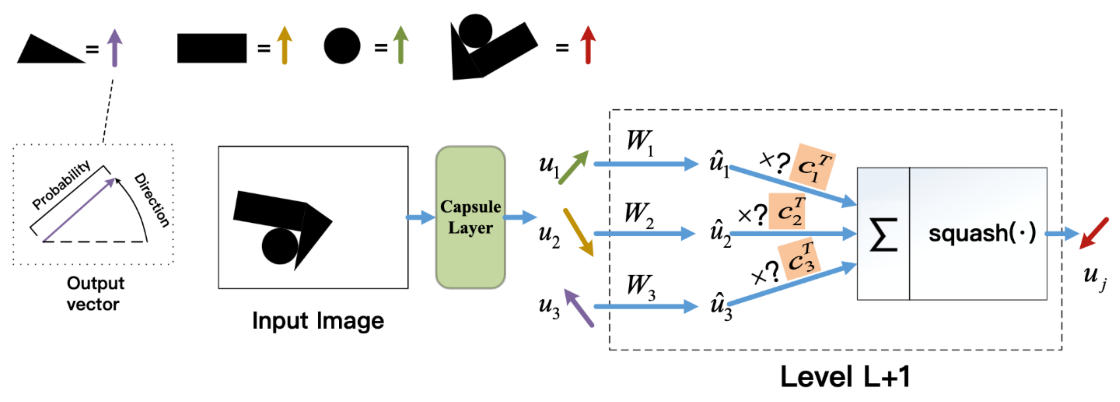
2. 2D Capsule Networks
3. 3D Mesh Capsule Networks
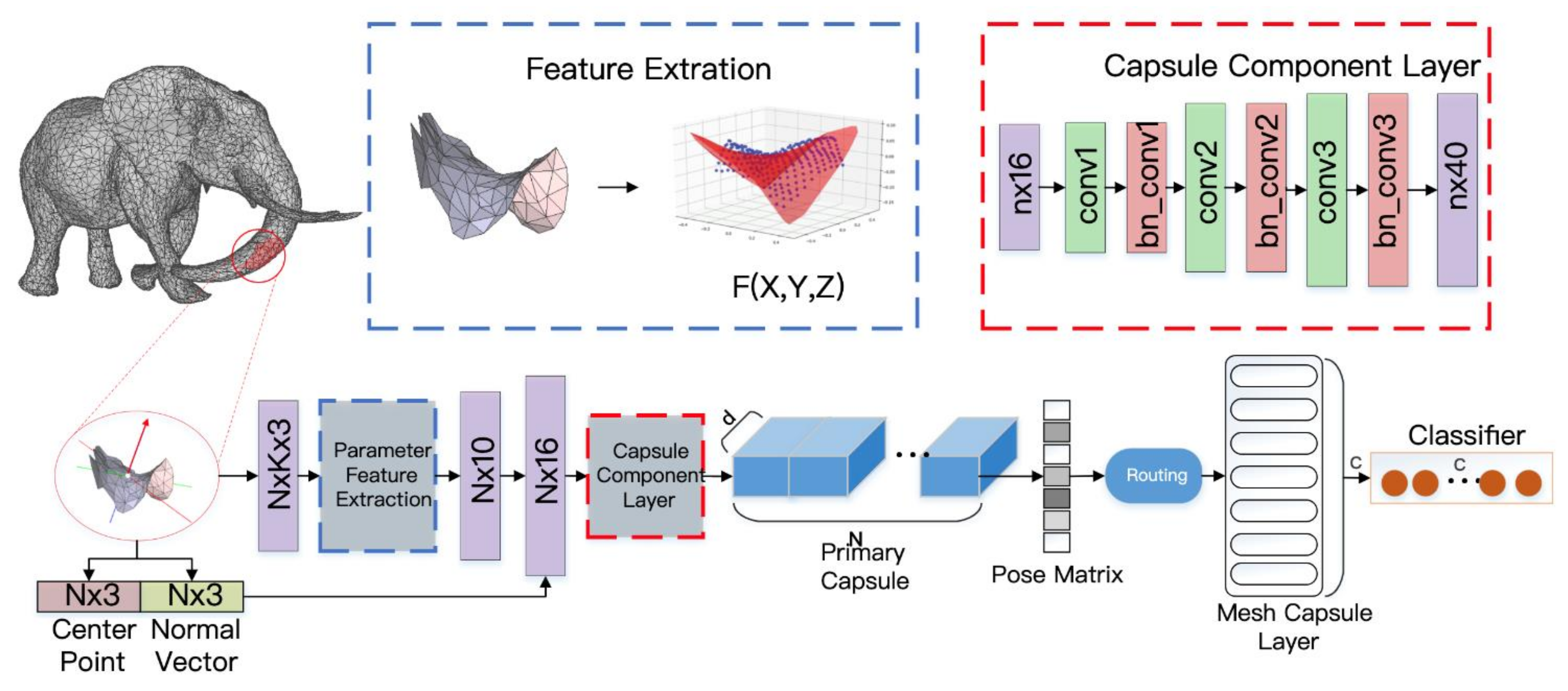
3.1. MeshCaps Framwork
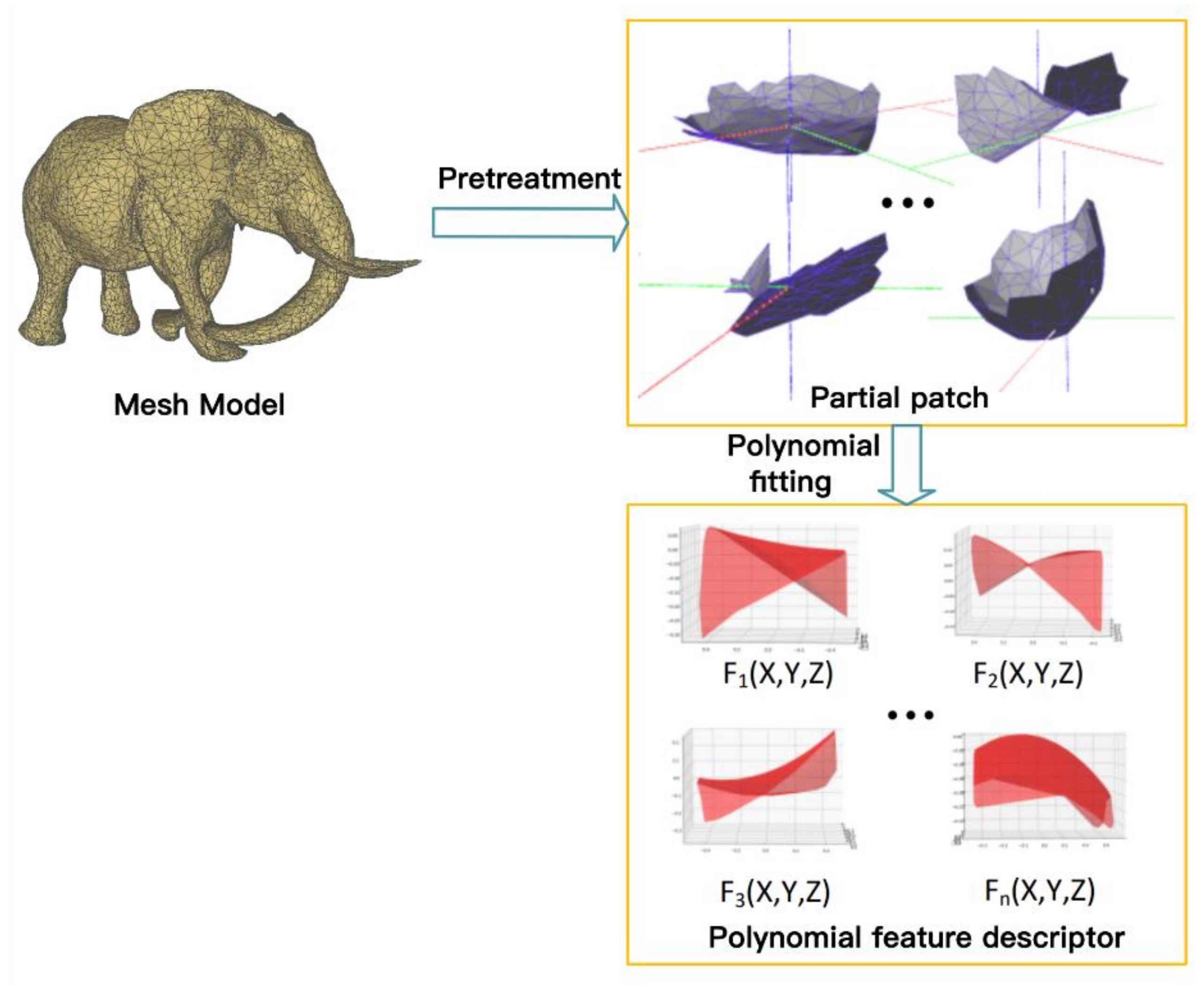
3.2. Local Shape Feature Extraction
3.3. Mesh Capsule Networks
4. Experimental Evaluation
4.1. Model Details
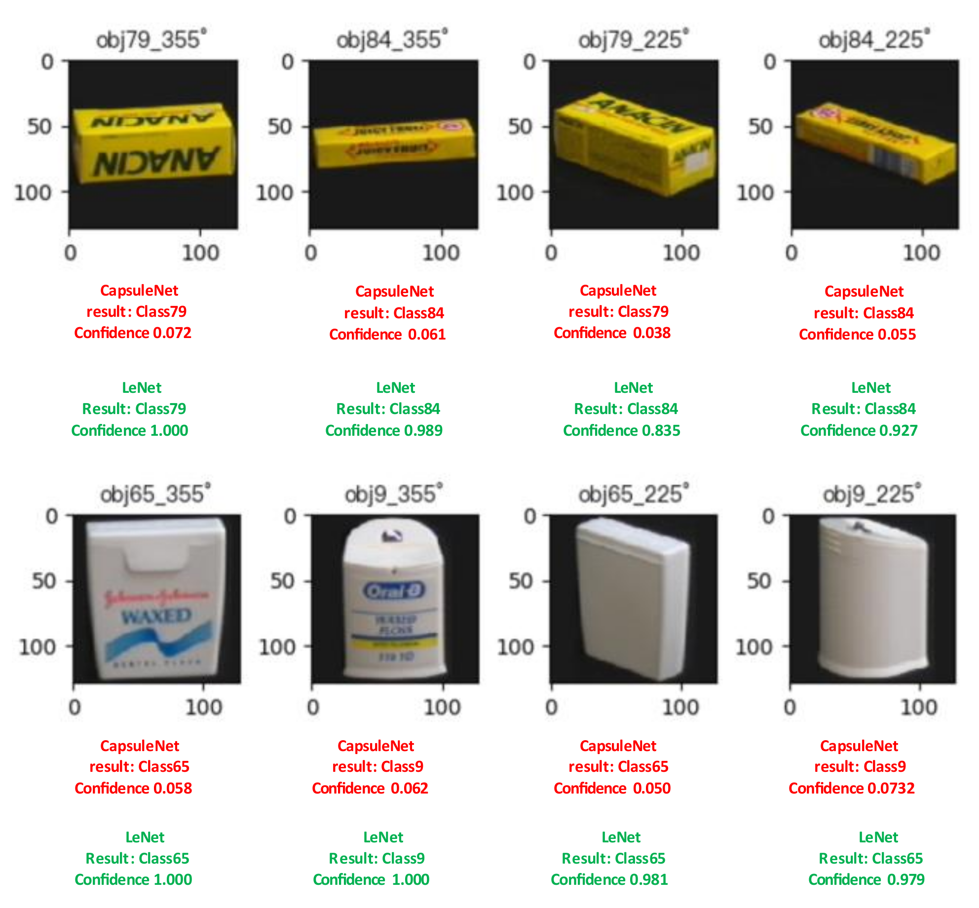
4.2. Accuracy Test
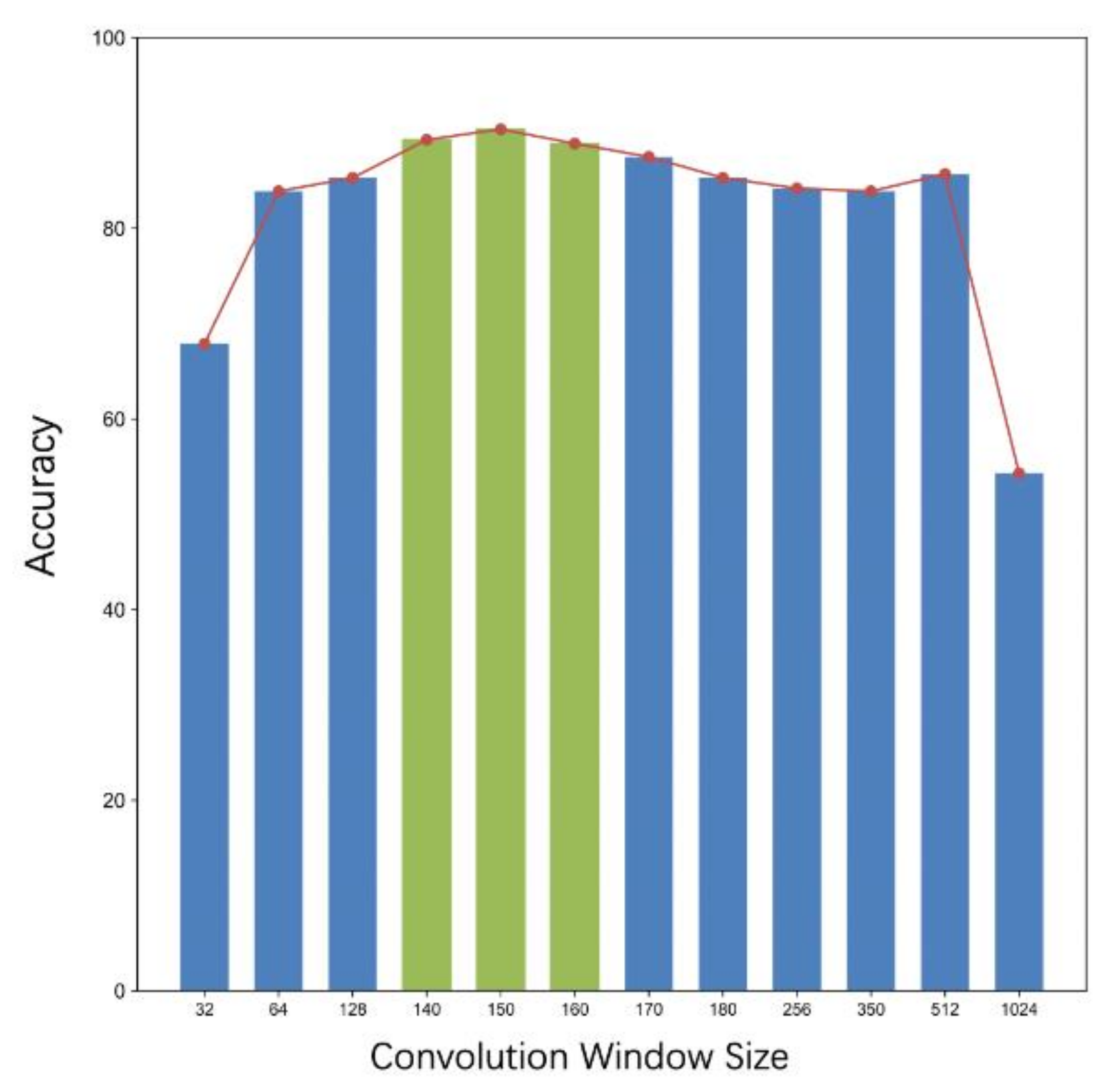
4.3. Convolution Window Size
4.4. Model Complexity Comparison
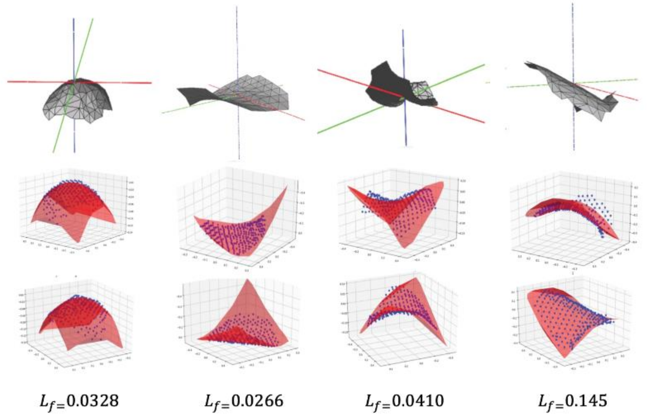
4.5. Influencing Factor Experiment
5. Conclusions
Author Contributions
Funding
Data Availability Statement
Conflicts of Interest
References
- Xie, Z.-G.; Wang, Y.-Q.; Dou, Y.; Xiong, Y. 3D feature learning via convolutional auto-encoder extreme learning machine. J. Comput. Aided Des. Comput. Graph. 2015, 27, 2058–2064. (In Chinese) [Google Scholar]
- Wu, Z.; Song, S.; Khosla, A.; Yu, F.; Zhang, L.; Tang, X.; Xiao, J. 3d shapenets: A deep representation for volumetric shapes. In Proceedings of the IEEE Conference on Computer Vision and Pattern Recognition, Boston, MA, USA, 7–12 June 2015. [Google Scholar]
- Maturana, D.; Scherer, S. Voxnet: A 3d convolutional neu-ral network for real-time object recognition. In Proceedings of the Intelligent Robots and Systems (IROS), 2015 IEEE/RSJ International Conference on, Hamburg, Germany, 28 September–3 October 2015; pp. 922–928. [Google Scholar]
- Li, Y.; Pirk, S.; Su, H.; Qi, C.R.; Guibas, L.J. FPNN: Field probing neural networks for 3D data. In Proceedings of the Advances in Neural Information Processing Systems, Barcelona, Spain, 5–10 December 2016; pp. 307–315. [Google Scholar]
- Wang, D.Z.; Posner, I. Voting for voting in online point cloud object detection. In Proceedings of the Robotics: Science and Systems, Rome, Italy, 13–17 July 2015; p. 1317. [Google Scholar]
- Wang, P.; Liu, Y.; Guo, Y.-X.; Sun, C.-Y.; Tong, X. O-CNN: Octree-based Convolutional Neural Networks for 3D Shape Analysis. ACM Trans. Graph. 2017, 36, 11. [Google Scholar] [CrossRef]
- Qi, C.R.; Su, H.; Mo, K.; Guibas, L.J. Pointnet: Deep learning on point sets for 3D classification and segmentation. In Proceedings of the IEEE Conference on Computer Vision and Pattern Recognition, Honolulu, HI, USA, 21–26 July 2017. [Google Scholar]
- Qi, C.R.; Yi, L.; Su, H.; Guibas, L.J. Pointnet++: Deep hierarchical. feature learning on point sets in a metric space. Advances in Neural Information Processing Systems. arXiv 2017, arXiv:1706.02413. [Google Scholar]
- Hanocka, R.; Hertz, A.; Fish, N.; Giryes, R.; Fleishman, S.; Cohen-Or, D. MeshCNN: A network with an edge. ACM Trans. Graph. 2019, 38, 1–90. [Google Scholar] [CrossRef]
- Feng, Y.; You, H.; Zhao, X.; Gao, Y. MeshNet: Mesh. Neural Network for 3D Shape Representation. arXiv 2019, arXiv:1811.11424. [Google Scholar] [CrossRef]
- Yang, Y.; Liu, S.; Pan, H.; Liu, Y.; Tong, X. PFCNN: Convolutional Neural Networks on 3D Surfaces Using Parallel Frames. In Proceedings of the IEEE Conference on Computer Vision and Pattern Recognition, Online, 14, 15, 19 June 2020. [Google Scholar]
- Wang, J.; Wen, C.; Fu, Y.; Lin, H.; Zou, T.; Xue, X.; Zhang, Y. Neural Pose Transfer by Spatially Adaptive Instance Normalization. In Proceedings of the IEEE/CVF Conference on Computer Vision and Pattern Recognition, Seattle, WA, USA, 14–19 June 2020; pp. 5831–5839. [Google Scholar]
- Qiao, Y.L.; Gao, L.; Rosin, P.; Lai, Y.K.; Chen, X. Learning on 3D Meshes with Laplacian Encoding and Pooling. IEEE Trans. Vis. Comput. Graph. 2020. [Google Scholar] [CrossRef] [PubMed]
- Litany, O.; Bronstein, A.; Bronstein, M.; Makadia, A. Deformable shape completion with graph convolutional autoencod-ers. In Proceedings of the IEEE Conference on Computer Vision and Pattern Recognition, Salt Lake City, UT, USA, 18–22 June 2018; pp. 1886–1895. [Google Scholar]
- Zhang, X.; Luo, P.; Hu, X.; Wang, J.; Zhou, J. Research on Classification Performance of Small-Scale Dataset Based on Capsule Network. In Proceedings of the 2018 4th International Conference on Robotics and Artificial Intelligence (ICRAI 2018), Guangzhou, China, 17–19 November 2018; pp. 24–28. [Google Scholar] [CrossRef]
- Sabour, S.; Frosst, N.; Hinton, G.E. Dynamic routing be-tween capsules. In Proceedings of the Neural Information Processing Systems (NIPS), Long Beach, CA, USA, 4–9 December 2017. [Google Scholar]
- Hinton, G.E.; Krizhevsky, A.; Wang, S.D. Transforming auto-encoders. In Proceedings of the International Conference on Artificial Neural Networks (ICANN), Espoo, Finland, 14–17 June 2011; Springer: Berlin/Heidelberg, Germany, 2011. [Google Scholar]
- Ren, H.; Su, J.; Lu, H. Evaluating Generalization Ability of Convo-lutional Neural Networks and Capsule Networks for Image Classification via Top-2 Classification. arXiv 2019, arXiv:1901.10112. [Google Scholar]
- Iesmantas, T.; Alzbutas, R. Convolutional capsule network for classification of breast cancer histology images. In International Conference Image Analysis and Recognition (ICIAR); Springer: Berlin/Heidelberg, Germany, 2018; pp. 853–860. [Google Scholar]
- Jaiswal, A.; Abdalmageed, W.; Wu, Y.; Natarajan, P. Capsulegan: Generative adversarial capsule network. In Proceedings of the European Conference on Computer Vision (ECCV), Munich, Germany, 8–14 September 2018. [Google Scholar]
- Yang, M.; Zhao, W.; Ye, J.; Lei, Z.; Zhao, Z.; Zhang, S. Investigating capsule networks with dynamic routing for text classi-fication. In Proceedings of the Conference on Empirical Methods in Natural Language Processing (EMNLP), Brussels, Belgium, 31 October–4 November 2018; pp. 3110–3119. [Google Scholar]
- Nguyen, H.H.; Yamagishi, J.; Echizen, I. Capsule-forensics: Using capsule networks to detect forged images and videos. In Proceedings of the International Conference on Acoustics, Speech and Signal Processing (ICASSP), Brighton, UK, 12–17 May 2019; pp. 2307–2311. [Google Scholar]
- Bazazian, D.; Nahata, D. DCG-Net: Dynamic Capsule Graph Convolutional Network for Point Clouds. IEEE Access 2020, 8, 188056–188067. [Google Scholar] [CrossRef]
- Bazazian, D.; Parés, M. EDC-Net: Edge Detection Capsule Network for 3D Point Clouds. Appl. Sci. 2021, 11, 1833. [Google Scholar] [CrossRef]
- Zhao, Y.; Birdal, T.; Deng, H.; Tombari, F. 3D point capsule networks. In Proceedings of the IEEE/CVF Conference on Computer Vision and Pattern Recognition, Long Beach, CA, USA, 15–20 June 2019; pp. 1009–1018. [Google Scholar]
- Ahmad, A.; Kakillioglu, B.; Velipasalar, S. 3D capsule networks for object classification from 3D model data. In Proceedings of the 2018 52nd Asilomar Conference on Signals, Systems, and Computers, California, CA, USA, 28–31 October 2018; pp. 2225–2229. [Google Scholar]
- Lecun, Y.; Bottou, L. Gradient-based learning applied to doc-ument recognition. Proc. IEEE 1998, 86, 2278–2324. [Google Scholar] [CrossRef]
- Kazhdan, M.; Funkhouser, T.; Rusinkiewicz, S. Shape matching andanisotropy. ACM Trans. Graph. 2004, 23, 623–629. [Google Scholar] [CrossRef]


| Network | Alien | Ants | Cat | Dog1 | Hand | Man | Shark | Santa | Pliers | Glasses | Dog2 | Camel | Snake | Avg |
|---|---|---|---|---|---|---|---|---|---|---|---|---|---|---|
| SPH [28] | 87.4% | 86.2% | 90.4% | 89.3% | 88.6% | 89.1% | 90.2% | 89.4% | 87.1% | 89.9% | 86.7% | 88.1% | 87.9% | 88.2% |
| MeshNet [10] | 89.5% | 89.6% | 89.6% | 91.4% | 90.5% | 90.8% | 90.1% | 89.8% | 88.0% | 91.4% | 90.5% | 90.3% | 89.9% | 90.4% |
| MeshCNN [9] | 91.2% | 91.4% | 92.1% | 90.2% | 90.5% | 91.6% | 92.7% | 90.5% | 91.8% | 90.4% | 92.3% | 93.7% | 90.3% | 91.7% |
| Ours-MeshCaps | 92.7% | 91.2% | 91.9% | 92.4% | 94.2% | 92.8% | 93.0% | 92.9% | 94.1% | 90.2% | 95.3% | 92.3% | 95.0% | 93.8% |
| Window Size K | Acc |
|---|---|
| 140 | 89.3% |
| 142 | 91.8% |
| 144 | 91.6% |
| 146 | 92.2% |
| 148 | 92.9% |
| 150 | 93.0% |
| 151 | 93.3% |
| 152 | 93.8% |
| 153 | 93.5% |
| 154 | 92.8% |
| 156 | 93.0% |
| 158 | 92.2% |
| 160 | 91.9% |
| Network | Capacity (MB) | FLOPs/Sample (M) |
|---|---|---|
| MeshCNN [9] | 1.323 | 498 |
| MeshNet [10] | 4.251 | 509 |
| SPH [28] | 2.442 | 435 |
| Ours-MeshCaps | 3.342 | 605 |
| Network Structure | Acc |
|---|---|
| Feature+3-Layer CNN | 89.9% |
| Feature+LeNet | 90.8% |
| MeshCaps | 93.8% |
| Sample Percentage | Acc |
|---|---|
| 100% | 87.4% |
| 95% | 85.8% |
| 90% | 91.8% |
| 85% | 93.8% |
| 80% | 89.5% |
| 75% | 79.1% |
| 70% | 80.4%% |
| Network Structure | Acc | |
|---|---|---|
| Component layer | Feature fusion | |
| No | No | 91.2% |
| No | Yes | 91.9% |
| Yes | No | 92.3% |
| Yes | Yes | 93.8% |
Publisher’s Note: MDPI stays neutral with regard to jurisdictional claims in published maps and institutional affiliations. |
© 2021 by the authors. Licensee MDPI, Basel, Switzerland. This article is an open access article distributed under the terms and conditions of the Creative Commons Attribution (CC BY) license (http://creativecommons.org/licenses/by/4.0/).
Share and Cite
Zheng, Y.; Zhao, J.; Chen, Y.; Tang, C.; Yu, S. 3D Mesh Model Classification with a Capsule Network. Algorithms 2021, 14, 99. https://doi.org/10.3390/a14030099
Zheng Y, Zhao J, Chen Y, Tang C, Yu S. 3D Mesh Model Classification with a Capsule Network. Algorithms. 2021; 14(3):99. https://doi.org/10.3390/a14030099
Chicago/Turabian StyleZheng, Yang, Jieyu Zhao, Yu Chen, Chen Tang, and Shushi Yu. 2021. "3D Mesh Model Classification with a Capsule Network" Algorithms 14, no. 3: 99. https://doi.org/10.3390/a14030099
APA StyleZheng, Y., Zhao, J., Chen, Y., Tang, C., & Yu, S. (2021). 3D Mesh Model Classification with a Capsule Network. Algorithms, 14(3), 99. https://doi.org/10.3390/a14030099