Towards Understanding Clustering Problems and Algorithms: An Instance Space Analysis

Abstract

Various criteria and algorithms can be used for clustering, leading to very distinct outcomes and potential biases towards datasets with certain structures. More generally, the selection of the most effective algorithm to be applied for a given dataset, based on its characteristics, is a problem that has been largely studied in the field of meta-learning. Recent advances in the form of a new methodology known as Instance Space Analysis provide an opportunity to extend such meta-analyses to gain greater visual insights of the relationship between datasets’ characteristics and the performance of different algorithms. The aim of this study is to perform an Instance Space Analysis for the first time for clustering problems and algorithms. As a result, we are able to analyze the impact of the choice of the test instances employed, and the strengths and weaknesses of some popular clustering algorithms, for datasets with different structures.

1. Introduction

With increasing demand for techniques to automatically discover patterns in large datasets, the importance of clustering for data exploration and decomposing datasets into smaller and more homogeneous subsets has created a renewed interest in clustering algorithms [1]. Such algorithms stem from statistical approaches, optimization algorithms, fuzzy approaches, evolutionary algorithms and unsupervised machine learning (ML) methods. With so many algorithms available for clustering, it is an open question about which algorithm is best suited for a particular dataset. The selection of the most effective algorithm for solving a new problem instance based on its characteristics has been studied since the early 2000s in a branch of ML called meta-learning [2,3,4]. Typically, the meta-learning system receives as input a set of meta-examples representing learning problems and the performances of a portfolio of candidate algorithms used in their solution. Each meta-example stores a set of features that describe the problem, or meta-features and a target attribute that indicates either: the best evaluated algorithm for that problem; a ranking of the top performing algorithms; or the performance value achieved by one or more algorithms when solving the problem.

Studies in meta-learning and the algorithm selection problem have motivated a number of other meta-analyses’ proposals. One of them is the Instance Space Analysis (ISA) methodology, which has successfully been applied to various problems such as classification [5], forecasting [6] and anomaly detection [7], but not yet to clustering. The framework was originally developed to evaluate optimization problems [8,9] and to learn how the characteristics of problem instances affect the performance of algorithms. It maps the instances into a 2D space, which is built based on a set of meta-features and the performance of a set of algorithms. From this 2D instance space perspective, it is possible to visualize sets of easy and hard instances, as well as determine “footprints” of the algorithms, indicating their domains of competence and reliability. This provides rich information for revealing the best set of algorithms to be applied to a given instance to support automated algorithm selection. Finally, the sufficiency of existing benchmark test suites can be scrutinized, and new test instances can be generated at target locations in order to expand and diversify the instance space.

This paper applies ISA to a comprehensive study of clustering problems and algorithms for the first time. Our central focus is to study how measurable features of a clustering dataset (problem instance) affect a given clustering algorithm’s performance metric, and to objectively analyze the strengths and weaknesses of different clustering algorithms from the inspection of the instance space generated. The definition of a cluster in the literature is not unique, and each algorithm may adopt a different clustering criterion. The biases assumed by different algorithms will be better suited for the identification of some types of structures in a dataset. Nonetheless, a dataset may contain different types of structures and valid clusters within different granularities. The clustering problem has, therefore, several challenging aspects and may benefit from meta-analysis that relate the characteristics of the problem’s instances to the performance of the algorithms which may be used in their solution, such as those provided by the ISA framework. These are the insights that we seek in this study.

The challenges of clustering are naturally transmitted to the ISA instantiation we seek. Firstly, extracting meaningful meta-features from clustering problems has received little attention in the meta-learning community and has been the subject of recent pieces of work [10,11]. Here, we gather and introduce a set of meta-features aimed to reveal different types of structures on data. Since there are multiple clusters’ definitions, the selection of the clustering algorithms to be evaluated must be careful and include representatives with different biases, which we also tried to fulfill, despite focusing on popular partitional and hierarchical clustering algorithms. Finally, the lack of an expected response hampers the evaluation of the clustering algorithms’ results. There are various clustering validation indexes which can be used in this evaluation, but each one of them has a bias towards one particular cluster definition, which may favor some algorithms to the detriment of others. Therefore, we have combined multiple validation indexes in order to better assess the algorithms’ performances.

The remainder of this paper is organized as follows: In Section 2, we present a theoretical summary and previous studies on meta-learning and ISA. In Section 3, we describe the methodology of ISA for clustering. Section 4 presents the results of building an instance space for clustering from artificial datasets, as well as the discussions around the results. Section 5 summarizes the results obtained by including real datasets in the analysis. Conclusions and future work are presented in Section 6.

2. Background

Meta-learning can be interpreted as the exploration of meta-knowledge to obtain efficient models and solutions to new problems [12]. One of the first and seminal meta-learning contributions was developed by Rice [13]. In his work, the author deals with the problem of algorithm selection, i.e., the choice of an algorithm, among a set of options that is more appropriate to solve a particular instance of a problem [3]. 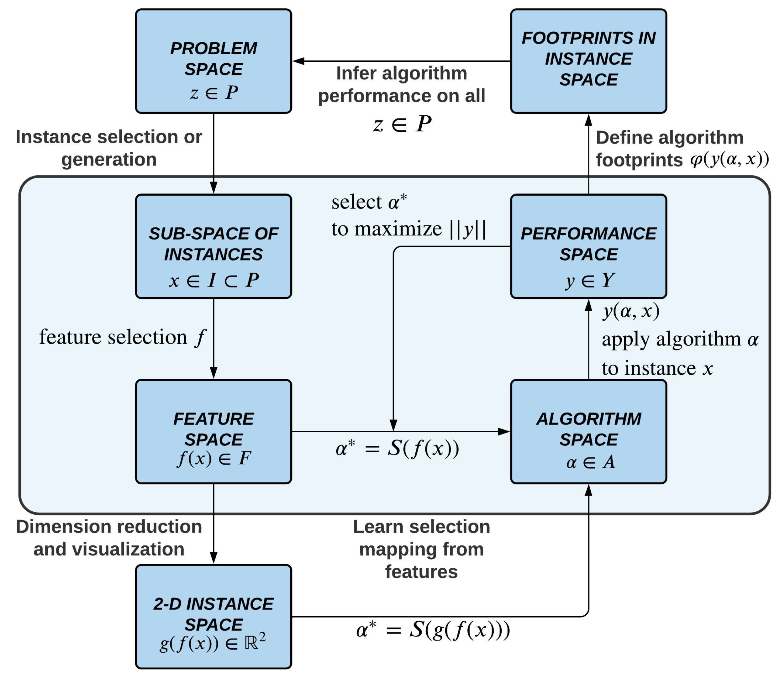Figure 1 illustrates Rice’s framework. Given a set of problem instances $x\in P$, from which measurable features $f\left(x\right)\in F$ are extracted, the objective is to learn a selection mapping $S\left(f\right(x\left)\right)$ to an algorithm ${\alpha }^{*}$ from a pool of candidate algorithms A which has optimized performance when solving x, as measured by a performance measure $y\in Y$.

Smith-Miles et al. [8] have extended Rice’s framework to propose a methodology known as Instance Space Analysis. Initially, the methodology was used to evaluate the suitability of algorithms for graph colouring problems, and later generalized to ML classification algorithms [5] and other problems [6,7,14]. According to Figure 2, the framework is composed of several steps. In the center, I contains a subset of the problem space P for which computational results are available. In ML, this subset is usually formed by datasets collected from benchmark repositories. The feature space F contains multiple measures that can be used to characterize the properties of the instances in I. The algorithm space A is composed of a portfolio of algorithms that can be used to solve the instances. The performance space Y measures the performance of the algorithms in A, when evaluated on the solution of the instances in I. Through a computational process, for all instances in I and all algorithms in A, a meta-dataset containing an ordered quadruple $(I,F,A,Y)$ is composed. One can then learn, through regression or another appropriate supervised learning method, the relationship between the features in F and the performance Y of the algorithms. This was the challenge of the Algorithm Selection Problem described by Rice [13] and shown in the inner box in Figure 2.

ISA methodology extends Rice’s framework to achieve more insights than mere algorithm selection. A 2D projection which captures relationships between the features values F and the performance measures Y can be generated. In this space, one may visualize the level of difficulty of different instances, the performance of different algorithms across the space and the relationship to instance features. The ultimate goal is more than automated algorithm selection, but greater insights into the strengths and weaknesses of algorithms, and explanations of how instance characteristics affect performance and reliability. Once the meta-data has been generated, the construction of the instance space involves a feature selection step in order to keep only the most informative meta-features and then projection of the instances into a 2D plane. Both of these steps require the solution of optimization problems: (i) to find the optimal subset of features that best explain variations in algorithm performance and “easy-to-hard” phase transitions; and (ii) to find the optimal linear transformation matrix from the selected feature space to 2D such that the distribution of algorithm performance and features in the 2D space exhibit strong linear trends for maximal visual interpretability.

The result is a projection of the instances into a 2D instance space that aims to elicit insights into why some algorithms might be more or less suited to certain types of instances. An ML model is applied to the instances in this space to learn algorithm “goodness”. Herewith, the regions where there is evidence of good performance are called the algorithm’s footprints, and represent a fundamental concept in ISA. The relative size of the footprints provide an objective measure of algorithm power, and their location indicates uniqueness and applicability to certain types of instances. The distribution of the instances also permits analysis of the diversity of the chosen benchmarks and opens up the possibility to generate new test instances that span underrepresented regions of the instance space. This was done in Muñoz and Smith-Miles [15] for generating custom classification datasets, through the fitting of a Gaussian Mixture Model and a set of generalized Bernoulli distributions, later refined in Muñoz et al. [5].

Lemke et al. [16] observe that, within the scope of ML, a considerable portion of the literature focuses on the use of meta-learning for algorithm recommendation. Regarding clustering problems, meta-learning has been explored as an alternative for clustering algorithm recommendation since the late 2000s [10,17,18,19,20,21]. Following a different perspective, Sáez and Corchado [22] developed a meta-learning system to determine the number of clusters in a dataset based on some quality indices. Pimentel and Carvalho [11] proposed a new data characterization method for selecting clustering algorithms, which was subsequently used in a meta-learning setup for recommending the number of clusters within a dataset [23]. Sallem and Gallagher [24] focus on landscape analysis of clustering problems viewed as black-box optimization problems, and solved using two well-known metaheuristics in clustering: Particle Swarm Optimization and Differential Evolution.

In a complementary meta-analysis perspective, the present work aims to analyse two aspects using ISA: (i) the diversity of clustering benchmarks; and (ii) the algorithmic power of some popular clustering algorithms.

3. Methodology of Instance Space Analysis for Clustering

The objective of clustering is to find structures in a dataset which summarize how the data points relate to each other in terms of their similarity of attributes. The resulting similarity structures or clusters can be found using statistical approaches, or unsupervised machine learning methods, and involve solving an optimization problem to allocate data points to clusters in a manner that maximises intra-cluster similarity and inter-cluster dissimilarity. There are several ways to define a cluster, resulting in different clustering criteria. In order to deal with such heterogeneity of approach, we first use different measures to characterize the clustering datasets, including meta-features used in previous works and also new measures that extract knowledge about the datasets’ structures according to different perspectives. In the evaluation of the algorithms, we combine various internal validation indexes in an average ranking. The objective of this combination is to embrace different clustering criteria, while also smoothing biases towards specific algorithms, which can happen between validation indexes and clustering algorithms employing similar clustering criteria. Furthermore, there are multiple challenges associated with clustering, mainly due to the lack of an expected output for the instances and the possible presence of multiple valid grouping structures on data. These challenges are also reflected in the construction of a suitable instance space for clustering instances, which must consider appropriate sets of instances, meta-features, algorithms, and evaluation measures. In this section, we describe the main steps followed in the generation of an instance space for clustering.

3.1. Clustering Instances and Algorithms

The first stage of the experiments used 380 synthetic clustering datasets from the literature to compose the instance set I. A total of 80 Gaussian datasets of low dimension and 80 ellipsoidal datasets of high dimension were collected from Handl and Knowles [25]. Another 220 datasets of various shapes and different number of attributes, clusters and instances from different sources were included [26,27,28,29,30,31,32,33,34,35,36,37,38,39,40,41,42]. In the selected datasets, the number of examples ranges from 100 to 5000, the number of attributes ranges from 2 to 1024 and the number of embedded clusters ranges from 1 to 40. Although we could include some labeled classification datasets into the analysis, as done in previous work [22,23], their structure is not always suitable for clustering purposes. For instance, there may be classes spanning different regions or manifolds of the input space. Additionally, a dataset might present more than one valid structure, which is not reflected in the assigned data labels. By employing synthetic datasets dedicated to the evaluation of clustering problems, we are able to circumvent these issues and build an instance space more suitable to clustering problems.

For composing the set of algorithms A, we analyzed 10 different partitional and hierarchical clustering algorithms widely used in the literature: K-Means (KME), K-Medians (KMD), K-Medoids (KMO), Mini-Batch K-Means (MBK), Fuzzy C-Means (FCM), Single Linkage (SL), Complete Linkage (CL), Average Linkage (AL), Closest Centroid (CC) and Ward’s Method (WM). The algorithms were executed using the implementations contained in the following R packages: stats, Gmedian, kmed, ClusterR and e1071. Appendix B presents the parameters used for each of the algorithms.

3.2. Meta-Data

An important step in the construction of meta-data are the definition of meta-features F that correspond to the characterization measures of the datasets.

Table 1. Meta-features classified by the main properties they measure. In the Asymp. column, n stands for the number of data items a dataset has and m corresponds to its number of input features.

Meta-Feature	Description	Asymp.	Reference
(1) Distribution-based:
multi_norm	Multivariate normality	$O(m·n+n^2)$	[17]
skewness	Multivariate normality skewness	$O(m·n+n^2)$	[43]
kurtosis	Multivariate normality kurtosis	$O(m·n+n^2)$	[43]
(2) Neighborhood-based:
avg_nnd	Average nearest neighbor degree	$O(m·n^2)$	[44]
contrast	Contrast	$O\left(n^2\right)$	[45]
high_dist	Percentage of points of high distance	$O\left(n^2\right)$	[10]
low_dist	Percentage of points of low distance	$O\left(n^2\right)$	[10]
(3) Density:
clust_coef	Clustering coefficient	$O(m·n^2)$	[46]
net_dens	Network density	$O(m·n^2)$	[46]
perc_out	Percentage of outliers	$O\left(n^2\right)$	[17]
(4) Dimensionality:
number_ex	${log}_{10}$ number of examples	$O\left(n\right)$	[17]
number_ftr	${log}_{10}$ number of attributes	$O\left(m\right)$	[18]
ratio_ex_ftr	Ratio number of examples to attributes	$O(m+n)$	[47]
avg_abs_cor	Average absolute correlation	$O\left(n\right)$	[20]
intr_dim	Intrinsic dimensionality	$O\left(n^2\right)$	[45]
avg_pca	Average number of points per PCA dimension	$O(m^2·n+m^3)$	[46]
ratio_pca	Ratio PCA to the original dimension	$O(m^2·n+m^3)$	[46]
(5) Network centrality:
power_cent	Bonacich power centrality	$O\left(n^3\right)$	[48]
eigen_cent	Eigenvalue centrality of minimum spanning tree	$O\left(n^2\right)$	[48]
hub_score	Kleinberg’s hub centrality	$O\left(n^3\right)$	[49]

lists the 20 meta-features used in this work. For each meta-feature, this table presents the main aspect it intends to measure, its acronym, description, asymptotic computational cost and reference from which the measure was extracted or based. The asymptotic cost is analyzed as a function of the number of points n each dataset has and its number of input features m. Most of the measures require building a distance matrix between all data points first, which dominates the asymptotic cost. Nonetheless, one must notice that this matrix needs to be computed only once and multiple measures can be extracted from it afterwards, so that the overall cost involved in extracting all meta-features is lower than that obtained by summing up each of the individual costs.

We have chosen a diverse set of meta-features for revealing different cluster structures while also allowing to draw meaningful conclusions regarding the clustering algorithm’s performances. Measures already tested in related works are included along with other measures that highlight other complementary aspects. The meta-features’ functions have been implemented in R, using the following packages as support: MVN and igraph. The code is available in an open access repository (see https://github.com/ml-research-clustering/meta-analysis, last accessed on 18 March 2021). They were categorized in this work in five groups, according to properties they are able to extract from the datasets: distribution-based, neighborhood-based, density-based, dimensionality and network centrality. Distribution-based, neighborhood-based and density-based measures are commonly employed as clustering criteria in the literature. Compact clusters are obtained whenever one maximizes the intra-cluster similarity, whilst minimizing inter-cluster similarity. Neighborhood-based measures favor placing neighborhood data items into the same group. Density captures how the data are distributed in the input space, so that dense regions separated by sparse regions can be regarded as suitable clusters. Dimensionality can be an issue to any clustering algorithm, as datasets with few data items and a high dimensionality tend to be sparse, which prevents finding an underlying clustering structure. The network centrality measures are based on building a proximity graph from data and measuring characteristics from this structure. The measures clust_coef and net_dens from the Density category and avg_nnd from the Neighborhood-based category are also extracted from this proximity graph. The graphs were built from the adjacency matrix, based on an approximation method that uses an $ϵ$-NN (nearest neighbor) function. As in related work [46], $ϵ$ is defined as 15% of the number of examples the dataset has. Finally, in our implementation, the percentage of points of high distance corresponds to the proportion of points with a distance greater than the mean distance plus its standard deviation. Conversely, the percentage of points of low distance corresponds to the proportion of points with a distance lower than the mean distance minus its standard deviation.

Some meta-features listed in Table 1 have already been used in previous work to characterize test instances in clustering problems [10,17,18,20,44,45,47]. We have also included some meta-features that have been used in classification problems that can be directly or easily adapted to characterize clustering problems [46]. As a contribution of this work, we have proposed using multivariate normality skewness and kurtosis measures [43] and a meta-feature group based on well-known network centrality measures [48,49]. The hypothesis is that the measurement of the importance of the vertices of a graph generated from the dataset reflects the structure of the clusters in such a way that it is possible to discriminate instances according to the underlying network complexity.

For evaluating the clustering algorithms’ performance and compose the set Y, we have employed a set of internal validation measures, which use information inherent to the data structure to assess the quality of the clusters [50,51,52,53,54,55,56,57,58]. There are numerous measures in the literature, each with a specific bias. The measures used in this work are classified in six groups, as shown in

Table 2. Performance measures classified by properties.

Acronym	Performance Measure	Reference
(1) Compactness or Homogeneity:
BH	Ball-Hall	[50]
(2) Connectedness:
C	Connectivity	[58]
(3) Separation:
RL	Ratkowsky–Lance	[54]
(4) Combinations:
CH	Calinski–Harabasz	[51]
DB	Davies–Bouldin	[55]
D	Dunn	[52]
SD	SD	[56]
(5) Stability:
APN	Average proportion of non-overlap	[57]
AD	Average distance	[57]
ADM	Average distance between means	[57]
FOM	Figure of merit	[57]
(6) Compliance between a partitioning and distance information:
HUB	Pearson correlation version of Hubert’s statistic	[53]

[58]. We included representatives from different categories as defined in the related literature, so that the ability of the algorithms to recover different structures from a dataset can be assessed. Their code was implemented in R, using the following packages: clusterCrit, clValid and fpc and are also available in supplementary material.

As a result of this step, we have a meta-dataset composed of 380 instances (clustering datasets), described by 20 meta-features and the performances of 10 clustering algorithms according to 12 clustering validation indexes.

3.3. Steps for Generating a 2D Instance Space for Clustering

The instance space is produced using the Matlab toolkit MATILDA (acronym for Melbourne Algorithm Test Instance Library with Data Analytics). MATILDA has been developed to be used in the analysis of optimization and ML problems (see https://matilda.unimelb.edu.au for a library of case studies, last accessed on 18 March 2021). A more detailed description of the methodology can be found in Muñoz et al. [5]. The tool consists of a data pipeline that integrates a pre-processing stage, four main steps and a post-processing stage.

A preliminary and relevant step to build an instance space is the consolidation of metadata. These are composed by the mentioned meta-features and performance measures of the algorithms under analysis. These actions are common in all kinds of problems, but in clustering some specific aspects had to be observed. The first is the need to determine an optimal number of clusters for each dataset. Considering the unsupervised nature of clustering problems, the number of clusters each dataset has is not known a priori. Therefore, we let the data structure speak for itself and the number of clusters is found according to the clustering algorithms’ results. We use the Silhouette Method [59] from the R language’s NbClust package to determine the number of clusters to be adopted for each dataset and clustering algorithm uniformly. It does not have the same bias of the internal validation criteria taken as performance measures. The inclusion of a new instance with or without information about the number of clusters must follow the same procedure.

Another aspect is the definition of a performance measurement. In this work, we chose to use internal validation measures because we did not want to consider the ground truths of the datasets. We know that there are countless measures and that each one has a specific bias and can favor a class of algorithms over others. To reduce this problem, we decided to select and combine measures adopting different clustering criteria. We grouped them into six groups according to Table 2. Each measure, or group of measures, has its own properties. To consider different biases, we aggregated them into a single value based on an average ranking of performance across the algorithm portfolio, in order to smooth or compensate their individual influence on algorithms which employ similar clustering criteria.

The first stage of the framework is the pre-processing of the meta-dataset. In this stage, the data were normalized using the Box-Cox and Z transformations. Next, a feature selection process is performed in order to find a subset of meta-features that are more related to the clustering algorithms’ performances, allowing for obtaining smoother 2D projections relating the properties of the instances and the performance of the clustering algorithms. MATILDA’s automated feature selection process defines the Pearson correlation coefficient as a similarity metric between features. K-means clustering is used to identify groups of similar features, with the number of groups defined by a Silhouette measure. K is a parameter that corresponds to a maximum number of clusters in the feature selection step. According to Appendix A, values were tested in the range 6–10. The value 10 was defined based on the tests. To select one feature per group, the algorithm first projects the subset of selected features into two dimensions using Principal Components Analysis (PCA) and Random Forests are used to predict whether an instance is easy or not for a given algorithm. Instances are labeled as easy or hard according to the performance threshold adopted for defining a good performance. In this work, we employed a threshold of 0.5, so that an instance for which an average ranking performance below 0.5 is achieved is classified as hard; otherwise, it is considered easy. Then, the subset of features that results in the most accurate Random Forest models is selected. This routine can be computationally intensive, since it tests all possible feature combinations if they are less than 1000 or uses the combination of a Genetic Algorithm and a look-up table otherwise.

Next, the main step for the generation of the instance space is the projection model. This algorithm was idealized as an optimization problem. It is a procedure of dimensionality reduction that projects the instances in a 2D space so that a linear trend is observed between the selected meta-features and the performance of the algorithms under analysis. The choice of projection to 2D is an experimental decision and any such dimensionality reduction produces a loss of information. Nevertheless, the use of 2D projection allows for visualizing better the distribution of the selected meta-features along the instance space and also of the algorithms’ performances variations. The 2D projection facilitates the computational requirements to establish the algorithm footprints too, corresponding to areas where the algorithms perform well. According to Muñoz et al. [5], given a (meta-)feature matrix $\mathbf{F}=[{\mathbf{f}}_1{\mathbf{f}}_2\cdots {\mathbf{f}}_3]\in {\mathbb{R}}^{m\times n}$ and algorithm performance vector $\mathbf{y}\in {\mathbb{R}}^n$ (which can also be generalized to a matrix containing multiple evaluations), where m is the number of features and n is the number of problem instances, we achieve an ideal projection of the instances if we can find ${\mathbf{A}}_{\mathbf{r}}\in {\mathbb{R}}^{2\times m}$, ${\mathbf{B}}_{\mathbf{r}}\in {\mathbb{R}}^{m\times 2}$ and ${\mathbf{c}}_{\mathbf{r}}\in {\mathbb{R}}^2$ which minimizes the approximation error

$$\begin{array}{c}\hfill \left|\right|\mathbf{F}-\widehat{\mathbf{F}}{\left|\right|}_F^2+\left|\right|{\mathbf{y}}^{\top }-{\widehat{\mathbf{y}}}^{\top }{\left|\right|}_F^2\end{array}$$

(1)

such that

$$\begin{array}{c}\hfill \mathbf{Z}={\mathbf{A}}_{\mathbf{r}}\mathbf{F}\end{array}$$

(2)

$$\begin{array}{c}\hfill \widehat{\mathbf{F}}={\mathbf{B}}_{\mathbf{r}}\mathbf{Z}\end{array}$$

(3)

$$\begin{array}{c}\hfill {\widehat{\mathbf{y}}}^{\top }={\mathbf{c}}_{\mathbf{r}}^{\top }\mathbf{Z}.\end{array}$$

(4)

The problem was solved numerically by MATILDA using BIPOP-CMA-ES (Bi-population Covariance Matrix Adaptation Evolution Strategy) [5].

The next step was the use of a supervised learning meta-model for algorithm selection. MATILDA trains a series of SVM models that predict whether an algorithm will perform well or not for a given instance, given a threshold of good and bad performance, which was set as 0.5 in this work. SVMs are trained using the selected meta-features as inputs and the performance measurement of each algorithm as output. The implementation of SVM uses a Gaussian kernel. Their hyper-parameters are tuned by Bayesian Optimization. The model uses a stratified k-fold cross-validation technique and gives a probability for each instance of belonging to a given class by fitting a posterior probability model ($k=5$ by default).

A central concept in ISA are the footprints, which represent the areas in the instance space where an algorithm is expected to perform well. The areas are calculated by Delaunay triangulation, considering the removal of contradictory evidence. For each of these areas’ measures of density, which would be the number of instances per unit area, and purity, which would be the number of instances of good performance per number of instances in the region, are extracted. When areas of two or more algorithms overlap, the purity measure is used to determine which algorithm should predominate.

Table A1. MATILDA parameters.

Parameter	Description	Test Range	Final Value
opts.perf.MaxPerf	True if Y is a performance measure to maximize, false to minimize	default	true
opts.perf.AbsPerf	True if an absolute performance measure, false if relative	default	true
opts.perf.epsilon	Threshold of good performance	0.30–0.80	0.50
opts.general.betaThreshold	Beta-easy threshold	0.45–0.75	0.50
opts.auto.preproc	Automatic preprocessing on	default	true
opts.bound.flag	Bound the outliers	true/false	false
opts.norm.flag	Normalize/Standardize the data	true/false	true
opts.auto.featsel	Automatic feature selection on	default	true
opts.corr.flag	Run feature selection by correlation between performance and features	default	true
opts.corr.threshold	Top N features (by correlation) per algorithm that are selected	default	10
opts.clust.flag	Run feature selection by clustering	default	true
opts.clust.KDEFAULT	Default maximum number of clusters	6–10	10
opts.clust.SILTHRESHOLD	Minimum accepted value for the average silhouette value	0.50–0.80	0.70
opts.clust.NTREES	Number of trees for the Random Forest	default	50
opts.clust.MaxIter	Maximum number of iterations	default	1000
opts.clust.Replicates	Number of replicates	default	100
opts.pilot.analytic	Calculate the analytical or numerical solution	default	false
opts.pilot.ntries	Number of attempts carried out by PBLDR	default	10
opts.cloister.pval	Maximum correlation coefficient	default	0.05
opts.cloister.cthres	Threshold of non-correlation	default	0.70
opts.pythia.cvfolds	number of folds of the stratified cross-validation partition	default	5
opts.pythia.useweights	weighted (true) or unweighted classification is performed	default	false
opts.trace.usesim	Use the actual or simulated data to calculate the footprints	default	true
opts.trace.RHO	Density threshold	default	5
opts.trace.PI	Purity threshold	default	0.55
opts.selvars.smallscaleflag	True if you want to do a small scale experiment	default	false
opts.selvars.smallscale	Percentage of instances to be kept for a small scale experiment	default	0.50
opts.selvars.fileidxflag	Activates selection by indexing	default	false
opts.selvars.fileidx	Name of a .csv file that contains in one column the indexes of the instances to be taken	default	“ ”
opts.outputs.web	Output files employed to draw the figures in MATILDA’s web tools	default	false
opts.outputs.png	Output as figures files for post-processing and analysis	default	true

in Appendix A shows the MATILDA parameter values adopted in this work. Most of the values adopted are default. Others were varied and the resulting projections were inspected for choosing suitable values. This examination is necessary to find a projection allowing for discriminating better the algorithm’s performances, whilst also showing smooth trends concerning the meta-features and algorithms’ performance values across the instance space. The aim of ISA is to gain insights and, if the parameters are not set suitably, few insights are available. For example, if the goodness threshold is not carefully chosen, all algorithms could be labeled good, and there will be little opportunity to allow ISA to distinguish strengths and weaknesses. While the default parameter settings in MATILDA have been chosen through many years of testing a variety of problems (see matilda.unimelb.edu.au for the collection of library problems, last accessed on 18 March 2021), there is still sometimes a need to explore a range of parameters to ensure the most insightful results are produced. In this study, experiments were conducted exploring different thresholds related to algorithmic performance and the selection of meta-features to arrive at some insightful visualisations, but the chosen parameters are quite robust.

4. Building an Instance Space from Artificial Datasets

All off the pre-processing steps of MATILDA were performed, with the exception of outlier detection. Experimental tests revealed that the exclusion of outliers reduced the quality of the projection in terms of the distribution of the instances in the 2D space, impairing the discrimination of the algorithms’ performances. All codes were executed on an Intel Core i7-7500U CPU with 2.70 GHz (Santa Clara, CA, USA), 16 GB RAM, and the Microsoft Windows 10 operating system (Redmond, WA, USA). The clustering algorithms ran once using their default parameter values (The code and datasets can be found at https://github.com/ml-research-clustering/meta-analysis, last accessed on 18 March 2021), except for the assumed number of clusters, which was adjusted to each dataset according to the Silhouette Method [59] from the NbClust R package. There are two details of implementation that deserve to be mentioned, both related to parameters of the employed function. First, the number of clusters to be considered was limited between the minimum and maximum values of the actual numbers of clusters all datasets from a given group contain. These limits were imposed to reduce the search space and the algorithmic runtime, since we are dealing with a large amount of datasets. If ground truths are not available, the minimum and maximum values can be set from 2 to $n-1$, where n is the size of the dataset. Secondly, the clustering algorithm used is varied among: K-Means, K-Medians, Closest Centroid, Single Linkage, Complete Linkage, Average Linkage, Ward, and McQuitty methods.

4.1. An Average Ranking for Performance Measures

As previously described, the internal validation indexes listed in Table 2 were aggregated into a single measure by taking an average ranking of performance of the algorithms (avg_rank). The idea is to combine multiple performance views of the clustering algorithms. The ranking uses the rank function of R. It is calculated as follows: (i) for each performance measure and dataset, a ranking of the algorithms is made, so that algorithms with better performance receive a better position in the rank compared to algorithms of lower performance; (ii) Then, the average and standard deviation of the ranking positions assigned to each algorithm are calculated. Standardization based on median and median deviation was applied to the ranking results, as well as Min-Max normalization. As a result, the ranking values range between 0 and 1, with larger values corresponding to better results.

All test instances were included in the analysis, divided according to the geometric shape of the clusters when projected in a 2D space. They were categorized into Gaussian, ellipsoidal or multiple shapes. The algorithm performance metric considered absolute performance, with a good performance identified when an algorithm reaches an avg_rank performance metric greater than or equal to $0.50$ for the given instance. This value corresponds to the threshold of good performance (opts.perf.epsilon). According to Appendix A, this parameter was varied in the range of 0.30–0.80. Adjusting this parameter allows for obtaining a projection that discriminates the performance of the algorithms better and makes it possible to visualize their footprints, that is, the regions of the space of instances in which the algorithms achieve good performance.

As mentioned earlier, MATILDA has the option of using a clustering-based feature selection method. It uses Pearson’s correlation coefficient as a measure of similarity and the k-Means algorithm to identify groups of similar features. The routine also embeds a silhouette analysis to infer the number of clusters and, therefore, the number of features to keep afterwards. A threshold of $0.70$ was used for the silhouette coefficient in this setting. According to Appendix A, this parameter was varied in the range 0.50–0.80. During execution, the MATILDA system itself recommends using a higher or lower value in order to obtain an optimized number of clusters in the feature selection process.

Table 3. Mean, standard deviation and rank of each clustering algorithm.

Algorithm	Mean	Std	Rank
CC	0.638	0.181	1
AL	0.629	0.174	2
SL	0.613	0.157	3
FCM	0.559	0.220	4
KME	0.551	0.177	5
CL	0.539	0.186	6
WM	0.522	0.209	7
KMD	0.521	0.203	8
MBK	0.476	0.182	9
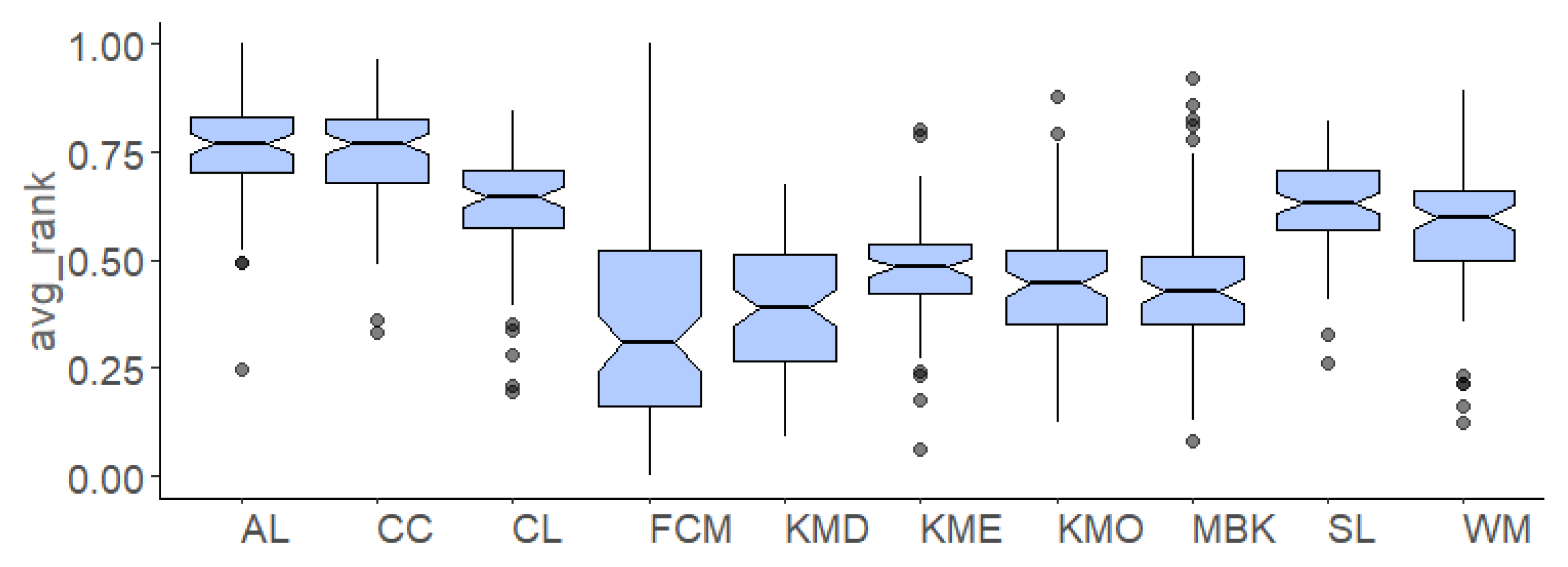
KMO	0.403	0.193	10

presents the mean and standard deviation of avg_rank measure across all test instances. The CC algorithm obtained the best average performance, while the KMO algorithm obtained less favorable results. Figure 3 further reveals that the partitional clustering algorithms performed poorly in the group of ellipsoidal datasets when compared with the hierarchical algorithms. The evidence found in these descriptive summary statistical results suggests that we should mostly rely on CC for a given clustering dataset, but does this algorithm have weaknesses? In addition, does the weakest algorithm, KMO, have hidden strengths that a more nuanced analysis would reveal? We aim to explore how ISA can fill this gap to gain greater insights than statistical averages can offer.

4.2. Feature Selection and Projection in the Instance Space

Ten meta-features were selected from the feature space F by MATILDA to be employed in the ISA analysis. Equation (5) presents the projection matrix that allows the transformation of instances from the 10D feature space to the 2D instance space. We can notice the presence of meta-features from all categories except from Network Centrality presented in Table 1, stressing the need for considering multiple views in order to properly characterize the structure of diverse datasets. Although no network centrality measures are present in the final set of meta-features chosen, the clust_coef meta-feature is also extracted from a proximity graph built from data.

$$\left[\begin{array}{c}\hfill Z_1\\ \hfill Z_2\end{array}\right]={\left[\begin{array}{cc}\hfill -0.124& \hfill 0.495\\ \hfill -0.572& \hfill 0.026\\ \hfill -0.147& \hfill -0.049\\ \hfill -0.231& \hfill 0.152\\ \hfill 0.435& \hfill -0.025\\ \hfill 0.505& \hfill -0.186\\ \hfill 0.154& \hfill -0.266\\ \hfill 0.205& \hfill 0.254\\ \hfill 0.131& \hfill -0.312\\ \hfill 0.007& \hfill -0.226\end{array}\right]}^{\top }\left[\begin{array}{c}\mathtt{ratio}\_\mathtt{ex}\_\mathtt{ftr}\\ \mathtt{skewness}\\ \mathtt{kurtosis}\\ \mathtt{perc}\_\mathtt{out}\\ \mathtt{ratio}\_\mathtt{pca}\\ \mathtt{avg}\_\mathtt{abs}\_\mathtt{cor}\\ \mathtt{low}\_\mathtt{dist}\\ \mathtt{clust}\_\mathtt{coef}\\ \mathtt{intr}\_\mathtt{dim}\\ \mathtt{avg}\_\mathtt{nnd}\end{array}\right]$$

(5)

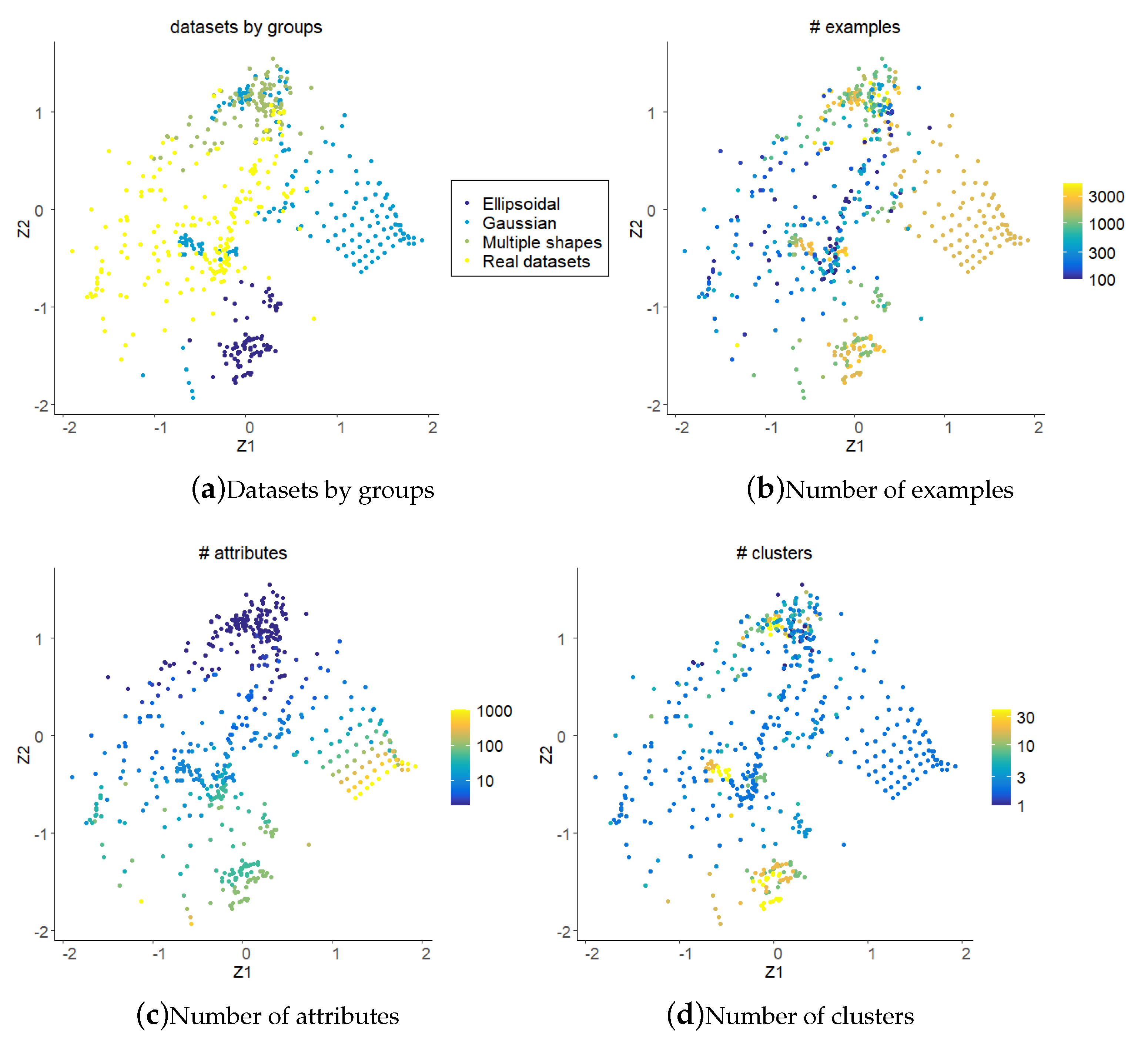
Figure 4 illustrates the characteristics of the 380 datasets projected in the generated instance space colored according to group (namely ellipsoidal, Gaussian and multiple shapes), number of examples, number of attributes and number of clusters defined as ground truth in the original datasets. There is a clear distinction between dataset groups. The ellipsoidal and multiply shaped datasets are spread in different regions of the instance space. Gaussian datasets occupy a region below them, with some degree of overlap. Among the Gaussian datasets, there is a set that is uniformly arranged in the lower region of the instance space. Those are the G2 datasets [42] that have the same number of observations (n = 2048), the same number of clusters (k = 2) and the number of attributes ranging from 2 to 1024. They also have an overlap parameter varying from 0 to 100. These datasets model each cluster as a separate Gaussian, which may or not overlap depending on the spread of their distributions.

We can see from the figure that the numbers of examples, attributes and clusters also are decisive in the distribution of datasets across the instance space. These characteristics were not directly used to project the instances, although the number of examples and attributes are used to compute some of the dimensionality measures. Datasets with more input attributes are concentrated in the bottom of the instance space, and their dimensionalities reduce towards the upper right quadrant of the projected space. For the number of clusters, although there are some mixed results, in general datasets with a lower number of clusters are concentrated towards the right of the instance space. Concerning the number of examples, datasets with fewer examples mostly have a $z_2$ coordinate larger than zero.

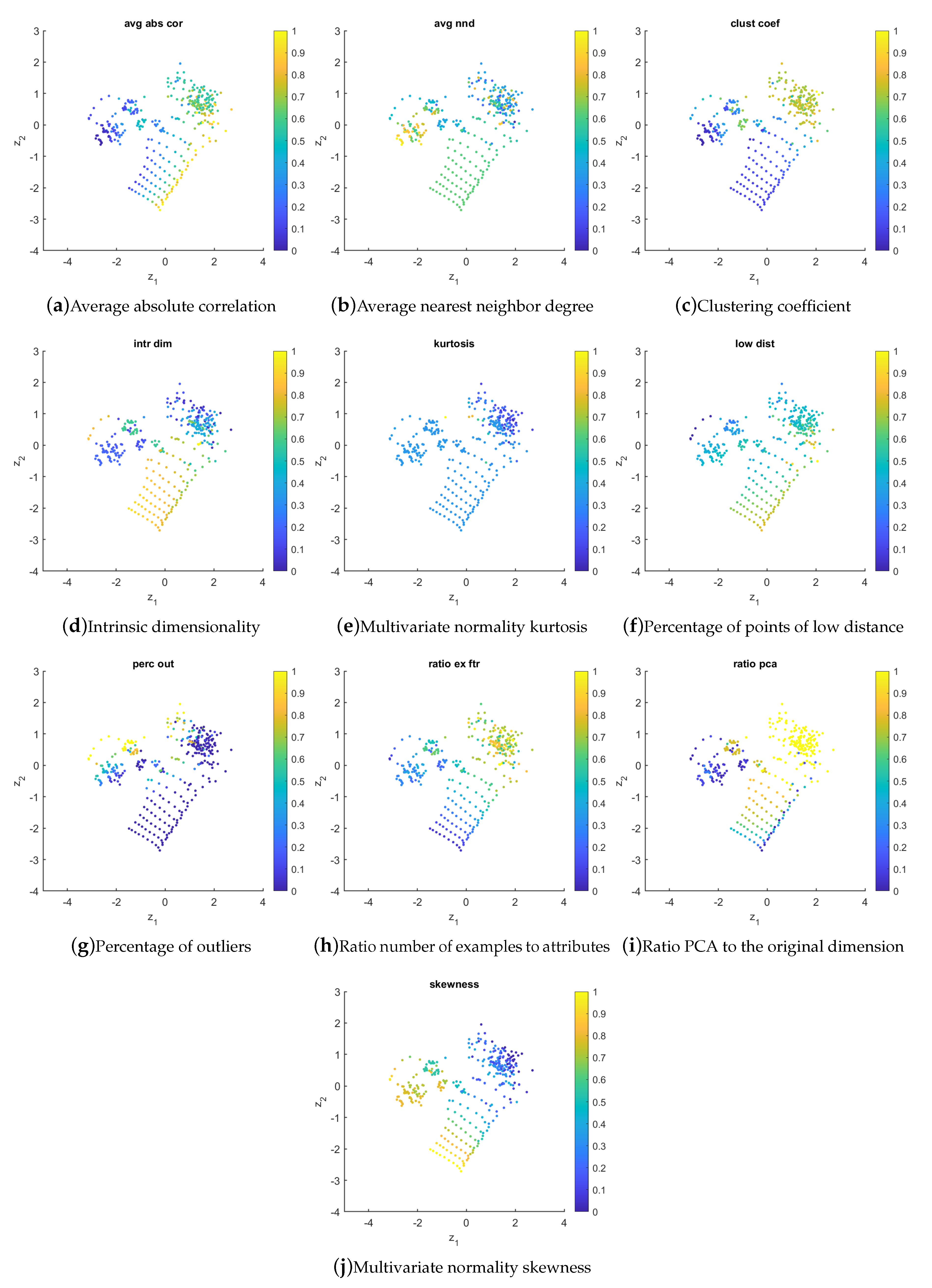
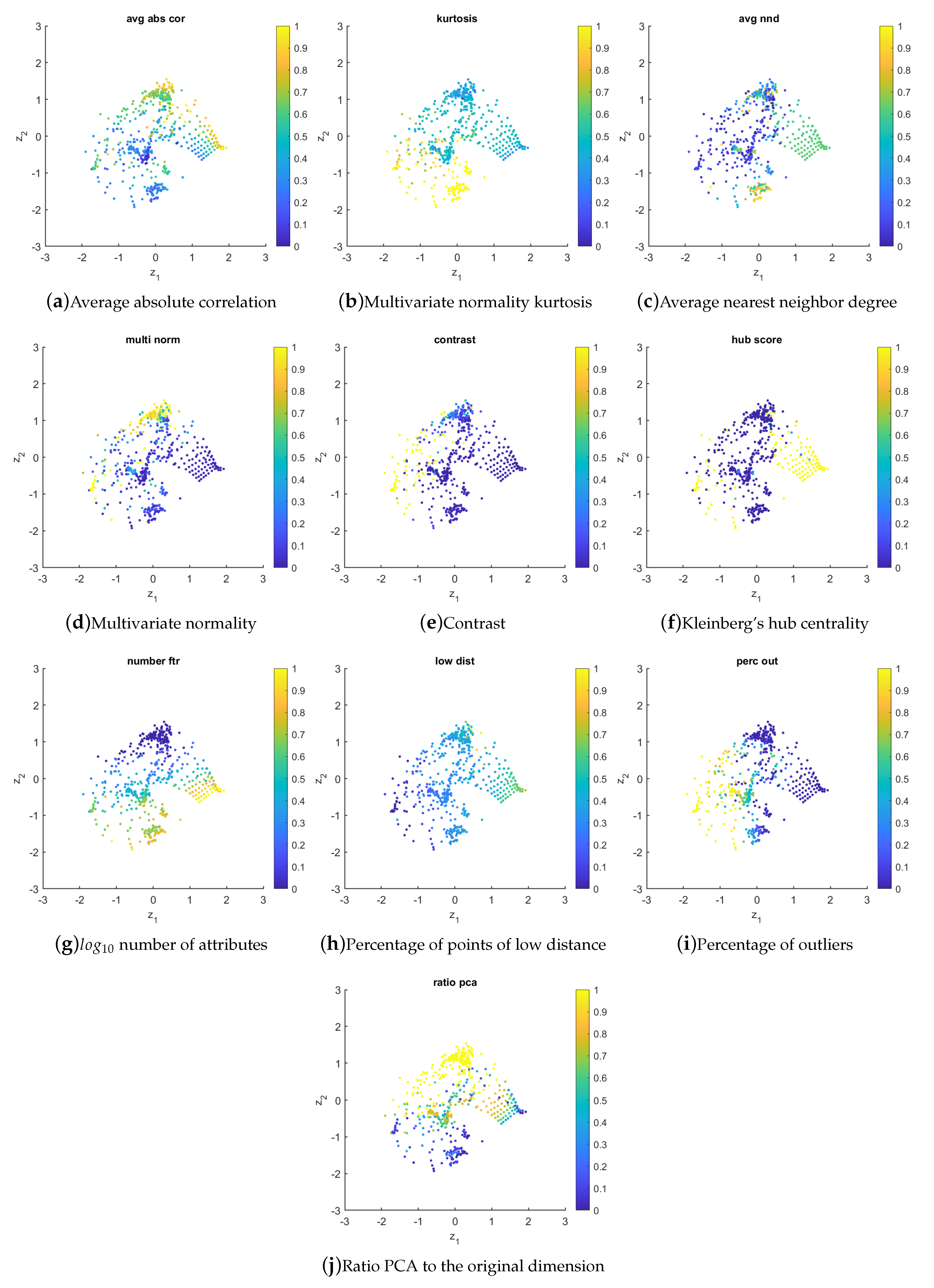
The distribution of the selected meta-features in the instance space is shown by Figure 5. All values were scaled to [0, 1]. In this case, the following observations can be drawn:

• avg_abs_cor: the values of this meta-feature increase from left to right in the instance space. This meta-feature computes the correlations between all input attributes a dataset has and averages their absolute values. Higher values are obtained for datasets with more redundant input attributes;
• avg_nnd: the values of this meta-feature tend to increase from right to left in the instance space. The degree captures more precisely the effective level of cohesiveness and affinity due to the actual interaction strength between nodes of the proximity graph built from a dataset [44]. A higher degree is expected for datasets with more examples near each other, so that the proximity graph shows more connections;
• clust_coef: the values of this meta-feature increase from bottom-left to the top-right of the instance space. The clustering coefficient of a vertex measures the ratio of the number of edges between its neighbors and the maximum number of edges that could possibly exist between them. A higher value is obtained for datasets with a more dense clustering structure;
• intr_dim: this meta-feature is characterized by having higher values for the G2 datasets. It measures the squared average distance between all points divided by the variance of the distances [45]. G2 datasets have a certain degree of overlap between clusters, justifying the higher values achieved;
• kurtosis: the values of this meta-feature tend to increase smoothly towards the bottom-left of the instance space. It calculates the Mardia’s multivariate kurtosis coefficient [43] of the dataset’s input attributes. A higher value reflects more complex datasets in terms of data distribution;
• low_dist: the values of this meta-feature tend to increase towards the bottom-right of the instance space. This measure computes the percentage of points with a distance lower than the mean distance between all data points in a dataset, minus its standard deviation. Higher values tend to be obtained for datasets with a greater degree of overlap between clusters;
• perc_out: the values of this meta-feature increase from bottom-right to the top-left of the instance space. In this work, outliers are considered points whose distance is less than $q_1-1.5d$ and higher than $q_3+1.5d$, where $q_1$ and $q_3$ are the first and third quartiles, respectively, and $d=q_3-q_1$. Essentially, this is an indicator of data quality that shows the ability of algorithms to deal with datasets that have non-uniform distribution;
• ratio_ex_ftr: the values of this meta-feature increase from bottom-left to the top-right of the instance space. This measure reflects the ratio between the number of examples and the number of attributes. It gives an indication of data sparsity, with lower values obtained for sparse datasets;
• ratio_pca: the values of this meta-feature tend to increase towards the up-right of the instance space. It is a rough measure of the proportion of relevant dimensions the dataset has, when compared to the number of principal components needed to represent 95% of data variability. High values of this measure indicate more complex relationships of the input variables [60];
• skewness: the values of this meta-feature tend to increase sharply towards the bottom-left of the instance space. It calculates the Mardia’s multivariate skewness coefficient [43]. A higher value reflects more complex datasets in terms of data distribution.

4.3. Algorithm Selection in the Instance Space—Performance Prediction

MATILDA uses SVM-based meta-models to predict in which regions of the instance space a particular algorithm would be the best choice for a given instance. Herewith, a specific module trains one SVM classification model per algorithm that predicts whether the algorithm will perform well or not for a given instance (see liveDemoIS.mlx file available at https://github.com/andremun/InstanceSpace, last accessed on 18 March 2021). It does this using the MATLAB fitcsvm package. In this process, the following operations are performed: (i) it produces resubstitution results using a stratified K-fold cross-validation (CV); (ii) it gives a probability for each instance of belonging to a given class, by fitting a posterior probability model; (iii) it uses Bayesian Optimization to fine tune the SVM hyper-parameters $\{C,\gamma \}$ that are the cost or regularization term and the radial-basis function kernel (RBF) hyper-parameter, respectively.

Table 4. Results of SVM prediction models, where Avg. Perf. is the Average Performance, SD Perf. is the Standard Deviation Performance, CV Accuracy, CV Precision and CV Recall are cross-validated performance metrics, C is the cost in the regularization term and $\gamma$ is the RBF hyper-parameter.

Algorithm	Avg. Perf.	SD Perf.	Prob. Good	CV Accuracy	CV Precision	CV Recall	C	$\mathit{\gamma }$
KME	0.55	0.18	0.62	74.70	75.90	86.30	206.99	1.34
KMD	0.52	0.20	0.59	78.70	78.90	87.60	3.82	0.28
KMO	0.40	0.19	0.35	71.80	72.60	33.30	554.32	4.53
MBK	0.48	0.18	0.43	73.20	85.40	46.10	79.39	4.56
FCM	0.56	0.22	0.67	90.00	87.70	98.80	97.26	0.45
SL	0.61	0.16	0.82	88.40	88.00	99.40	1.12	0.34
CL	0.54	0.19	0.63	75.00	77.30	85.40	5.23	0.83
AL	0.63	0.17	0.76	81.10	82.60	95.20	44.55	0.99
WM	0.52	0.21	0.55	80.30	80.10	85.10	0.44	0.38
CC	0.64	0.18	0.85	91.10	90.70	99.70	0.84	0.92
Oracle	0.81	0.09	1.00	-	-	-	-	-
Selector	0.67	0.14	0.91	-	91.30	47.70	-	-

shows the results obtained by the SVM predictors for each clustering algorithm (10 in total), as well as the results of an idealized oracle that always picks the right algorithm, and a selector that combines the decisions made by all the SVMs models to predict the likely best algorithm for each instance using the highest precision SVM to break ties. This assumes that the most precise SVM (CV-Precision) is the most reliable. The table includes the average and standard deviation of the performance measure across all instances (the average ranking obtained for all datasets), probability of good performance and 10-fold CV performance of the SVM models (accuracy, precision and recall). The SVM parameter values employed are also shown. The average ranking and its standard deviation are the expected performance if we were to use each algorithm across all instances. As already mentioned in the paper, the threshold for good performance defined in MATILDA was set as an avg_rank performance metric of at least $0.50$. The probability of good performance is based on this parameter and represents the fraction of instances for which the performance measure is greater than or equal to $0.50$. The clustering algorithm that presented the best performance on average was CC (probability of good 0.85), while the worst was KMO (probability of good 0.35). The results also indicate that the class of hierarchical algorithms in general presented better performance. The Selector is successful since it has a probability of 0.91 of selecting an algorithm with good performance and a CV-Precision of 91.30—better than always selecting the best on-average algorithm, which is CC (0.85). Nonetheless, the relatively low CV Recall of the Selector indicates that it could be further improved.

4.4. Footprint Analysis and Algorithm Portfolio

One of the most relevant and characteristic results of ISA is the presentation of the regions of the instance space in which the algorithms perform well, that is, the footprints of the algorithm, supporting objective evaluation of algorithmic power and highlighting its strengths and weaknesses. According to Muñoz et al. [5], the algorithm that generates the footprints uses a combination of two approaches that were used in previous works. In its first step, the algorithm measures the Euclidian distances between two instances, and marks one of them for elimination if the distance is less than a threshold, $\alpha$. This is done to avoid numerical instability with the triangulation algorithm, which is applied as the second step. As a third step, the algorithm finds the concave hull, by removing any triangle with edges larger than another threshold, $\beta$. As a fourth and final step, the algorithm calculates the density and purity of each triangle in the concave hull. The density, as the number of instances per area unit, and purity, as the number of instances of good performance (considering an avg_rank performance metric of at least 0.50) per number of instances of the region. If a triangle does not fulfill the density and purity limits, it is removed from the hull. When areas of two or more algorithms overlap, the purity measure is used to determine which algorithm should predominate. While we are not able to experiment with these default parameters, we can confirm that the resulting footprints make visual sense, and the parameters appear to behave in the intended manner, for our application, as well as all for the MATILDA library case studies. Changes to these parameters would merely affect the formation of footprints and the calculation of their areas, which is not a core requirement for gaining the visual insights we seek.

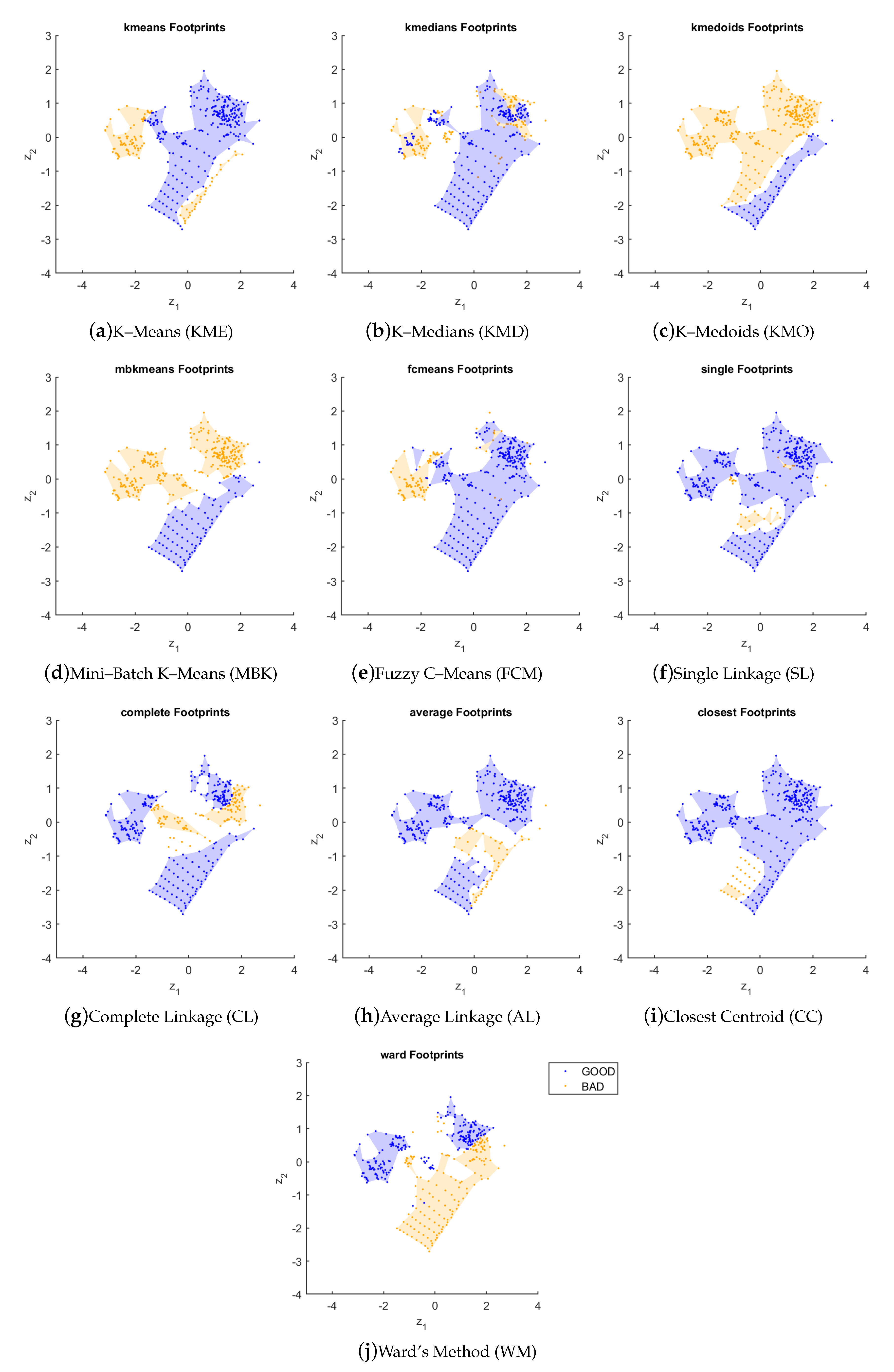
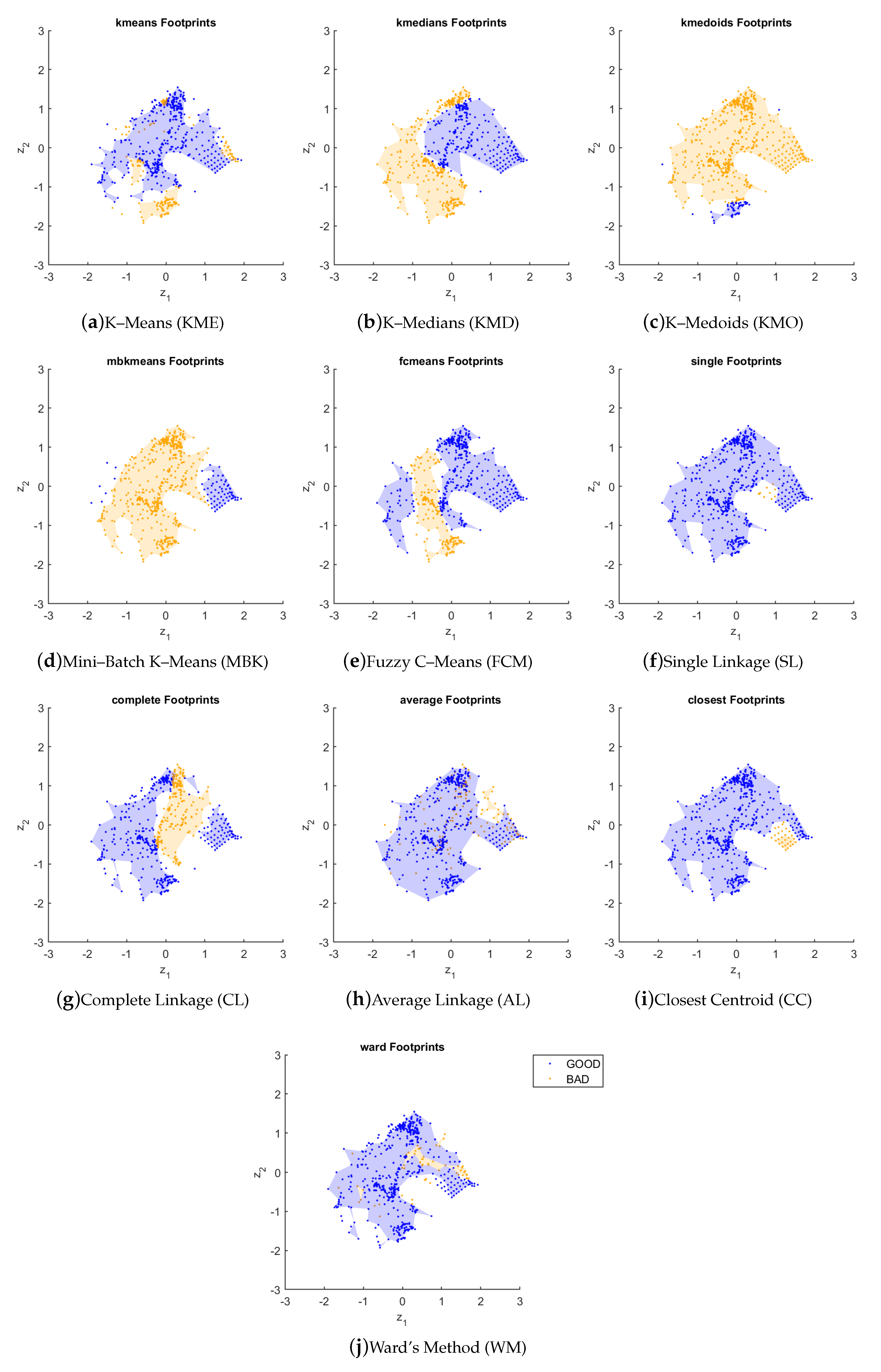
Figure 6 shows the footprints of the algorithms in the instance space. An interesting aspect to be observed is that all hierarchical algorithms perform well in the ellipsoidal datasets (center-left region), which are more complex in terms of some basic characteristics such as number of attributes and clusters. This was not observed for any of the partitional algorithms. We can also observe that the CC algorithm has the largest footprint in terms of coverage area across the instance space. On the other hand, the KMO algorithm has the smallest footprint area $\Delta$. Some other interesting observations from Figure 6 are:

• there is a large variation on the partitional algorithms’ performances, although all of them algorithms tended to present better results for datasets towards the bottom-right of the instance space, with exception from a small area in the case of KME. KMO and MBK present a large area of bad performance. The FCM variant is able to handle better a larger portion of the datasets;
• the hierarchical clustering variants tended to present bad results for some datasets of the G2 group;
• the WM algorithm presents a performance mostly complementary to that of the partitional algorithms.

Table 5. Footprint analysis of the algorithms, where $\Delta$ is the area, $\rho$ is the density and $\varphi$ is the purity.

Algorithm	$\mathbf{\Delta }$	$\mathit{\rho }$	$\mathit{\varphi }$
KME	0.71	0.97	1.00
KMD	0.70	0.89	0.89
KMO	0.19	0.80	1.00
MBK	0.35	0.66	1.00
FCM	0.78	0.96	0.98
SL	0.82	1.14	0.98
CL	0.54	1.26	1.00
AL	0.65	1.33	1.00
WM	0.27	1.98	0.99
CC	0.87	1.08	1.00

presents the results for the footprint analysis. The areas $\Delta$, as well as their density $\rho$ and purity $\varphi$ measures, are detailed. Usually, the obtainment of large normalized areas (30% onwards) with density about one and purity above 70–80% is evidence that the algorithm is strong in the instance space. The CC algorithm showed the best performance ($\Delta =0.87$), followed by the SL ($\Delta =0.82$) and FCM ($\Delta =0.82$). CC performed well on ellipsoidal, multiple shapes and Gaussian datasets, with the exception of a region formed by G2 datasets. SL obtained a similar result. FCM performed well in Gaussian datasets and multiple shapes, but did not obtain a good performance in ellipsoidal datasets. The worst performances were obtained by the KMO ($\Delta =0.19$), WM ($\Delta =0.27$) and MBK ($\Delta =0.35$) algorithms. The hierarchical algorithms in general showed better performance, which can be evidenced by the measures of area and density.

An important aspect in relation to ISA is the possibility of establishing a visual relationship between features and footprints, in order to highlight the strengths and weaknesses of the algorithms. A simultaneous analysis of Figure 5 and Figure 6 allows us to make the following statements about the relationships between datasets, meta-features and the performance of the algorithms:

• partitional algorithms results are directly related to ratio_pca, low_dist and avg_abs_cor, that is, those meta-features show where the algorithms perform well. On the other hand, their weaknesses are related to perc_out;
• regarding hierarchical algorithms, perc_out has a direct relationship with good performance, while avg_abs_cor and low_dist show the most difficult instances;
• similar relationships can also be verified when considering only the Gaussian datasets;
• in the group of ellipsoidal datasets, features avg_nnd and skewness show the strength of hierarchical algorithms, while features avg_abs_cor and clust_coef show their weaknesses;
• partitional algorithms do not have in general a uniform behavior for ellipsoidal datasets;
• in the group of multiple shapes, features ratio_pca, ratio_ex_ftr and clust_coef show the strength of hierarchical algorithms. KME, KMD and FCM present a direct relationship with those features, while KMO and MBK present an inverse relationship with perc_out;
• the best algorithm, CC, has its strengths evidenced by features clust_coef and ratio_ex_ftr, and weaknesses by features ratio_pca and low_dist;
• the worst algorithm, KMO, has its strengths evidenced by features low_dist and avg_abs_cor, and weaknesses by features perc_out and kurtosis.

We can conclude, therefore, that for the instances under study, the partitional and hierarchical algorithms in general tend to present inverse behaviors in relation to performance across the instance space.

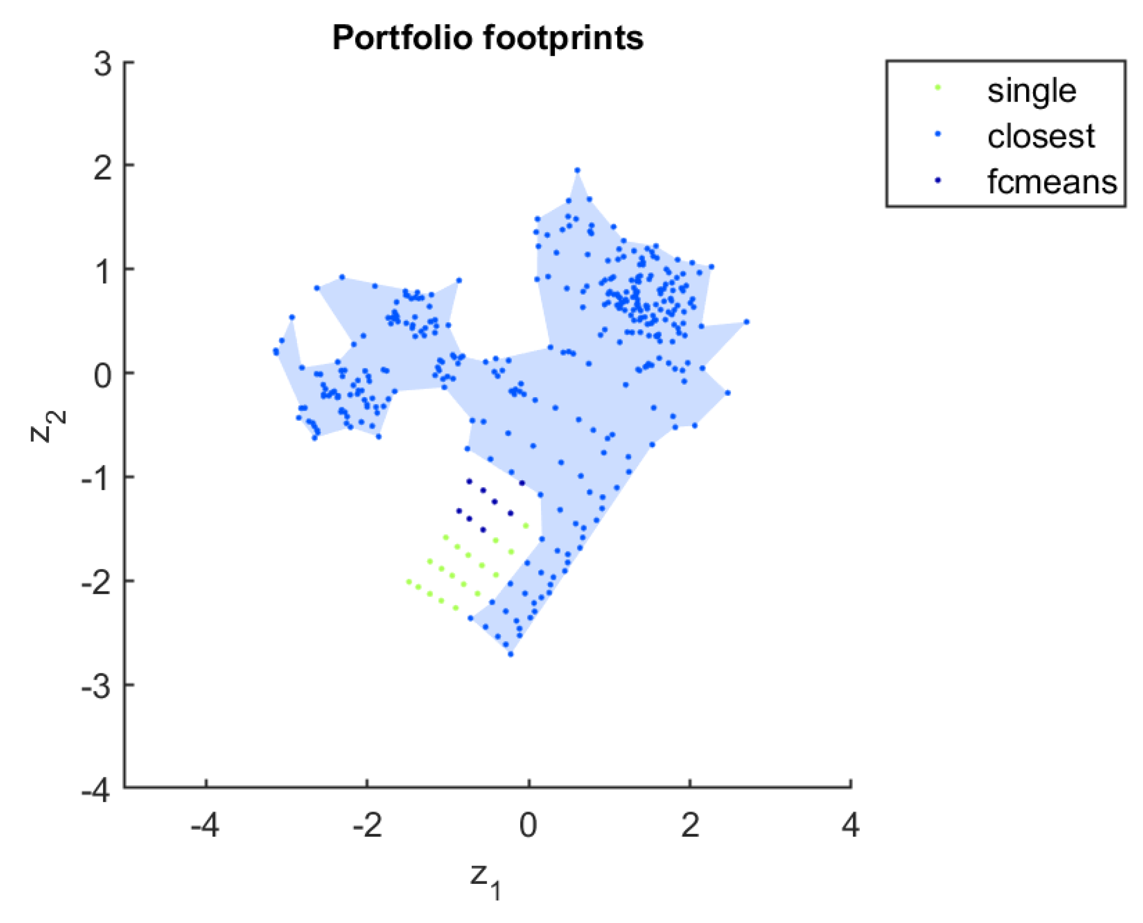
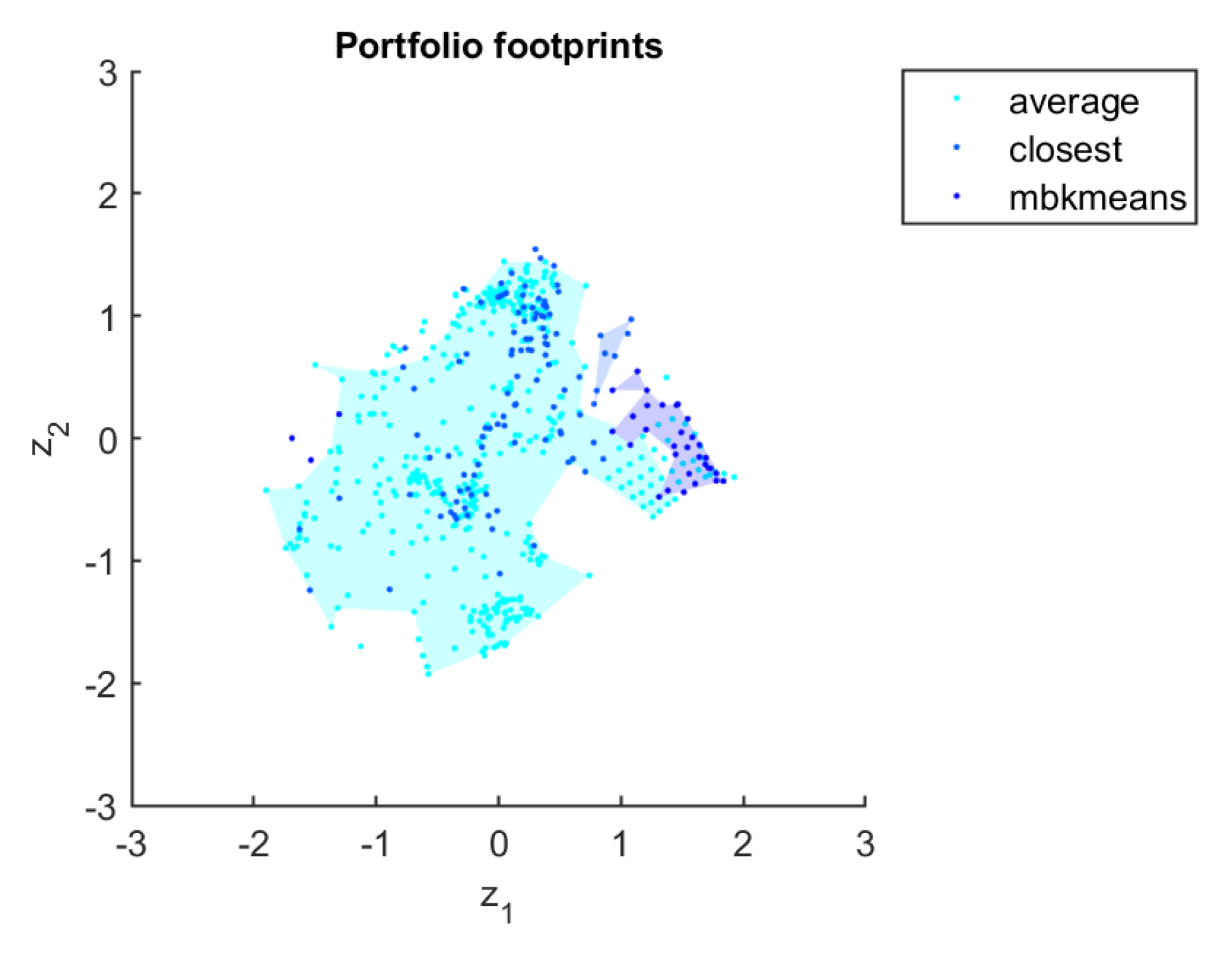
Figure 7 shows the footprints of the algorithm portfolio. The ISA’s results are consistent with those from the simple average performance analysis of algorithms, but with more nuanced insight possible. The SVM results recommend the CC algorithm for most instances of the three groups of datasets, but not all. There is also a recommendation for the SL and FCM algorithms in a small region of the Gaussian datasets.

5. Plotting Real Datasets in Instance Space

The instance space presented in the previous section was generated from artificial datasets with known clustering properties and structures. The adoption of this restriction resides in the fact that synthetic data allow a clearer and more objective understanding of the study results. They allow a more effective control over eventual relationships between selected meta-features and performance measures. However, reaching more comprehensive insights requires the use of datasets that reflect typical difficulties of real cases. We present in this section an ISA that incorporates real data, in order to verify in which regions of the instance space these datasets would be located and whether they influence the results obtained previously. This allows us to assess the difficulty level of real datasets and to examine the real-world-likeness of synthetic datasets. Only the main findings are highlighted, given that the details of the methodology employed are the same and have already been described in Section 3.

5.1. Generating an Instance Space from Combined Artificial and Real Datasets

A new instance space was generated from a total of 599 datasets, where 380 are the same artificial datasets used in Section 3 and another 219 real datasets were collected from the OpenML repository and used as benchmark for clustering algorithms in [11]. In these datasets, the number of examples ranges from 100 to 5000, the number of attributes ranges from 2 to 168, and the number of embedded clusters ranges from 2 to 30. One must notice that these datasets are representatives of classification problems. In classification problems, the objective is to find a decision model able to partition the data items into some previously defined categories. The datasets are then labeled and the model is trained to somewhat reproduce such labels. A same class can have data points spanning different regions of the input space. This differs from clustering, in which there are no pre-defined categories and the groups are usually based on their proximity. Whilst a problem for which the instances are distributed uniformly all over the input space with a clear linear decision border between the classes can be considered quite easy for classification, this is not the case for clustering (in fact, there is no cluster structure for data points randomly distributed in the input space). Therefore, although the usage of classification datasets in the evaluation of clustering algorithms is largely employed, some care must be taken in the interpretation of the obtained results.

The ground truths of the real datasets were not considered in the analysis. The same procedure used with artificial datasets was employed: the clusters were defined by the Silhouette method, using the implementation of the NbClust package from R. The categorization of artificial datasets described in the previous section has remained unchanged (namely ellipsoidal, Gaussian and multiple shapes). Equation (6) presents the new projection matrix. We can see that 10 meta-features were selected. A total of six remained in the projection matrix after the inclusion of the real datasets: kurtosis, perc_out, ratio_pca, avg_abs_cor, low_dist and avg_nnd. This indicates that these measures have a relevant influence in the characterization of both types of datasets.

$$\left[\begin{array}{c}\hfill Z_1\\ \hfill Z_2\end{array}\right]={\left[\begin{array}{cc}\hfill 0.110& \hfill -0.249\\ \hfill -0.084& \hfill -0.195\\ \hfill -0.201& \hfill 0.094\\ \hfill -0.270& \hfill -0.157\\ \hfill 0.071& \hfill 0.287\\ \hfill 0.178& \hfill 0.224\\ \hfill 0.197& \hfill 0.019\\ \hfill -0.197& \hfill 0.013\\ \hfill 0.163& \hfill 0.023\\ \hfill 0.077& \hfill -0.132\end{array}\right]}^{\top }\left[\begin{array}{c}\mathtt{number}\_\mathtt{ftr}\\ \mathtt{kurtosis}\\ \mathtt{multi}\_\mathtt{norm}\\ \mathtt{perc}\_\mathtt{out}\\ \mathtt{ratio}\_\mathtt{pca}\\ \mathtt{avg}\_\mathtt{abs}\_\mathtt{cor}\\ \mathtt{low}\_\mathtt{dist}\\ \mathtt{contrast}\\ \mathtt{hub}\_\mathtt{score}\\ \mathtt{avg}\_\mathtt{nnd}\end{array}\right]$$

(6)

Figure 8 shows the characteristics of the datasets projected in the instance space. The number of clusters for the real datasets correspond to their number of classes. Figure 9 and Figure 10 show the distribution of selected meta-features and algorithms footprints in the instance space, respectively.

Figure 8 reveals the region of the instance space where the real datasets were plotted. They are concentrated in the central and upper left region of the instance space, partially overlapping the less complex Gaussian datasets and the multiple shapes datasets. They also fill a central and lower left area not occupied by artificial datasets, which is characterized by a reduced number of examples and intermediate number of attributes and clusters. With very few exceptions, we can verify that, in general, they are not located in the areas occupied by the ellipsoidal and the G2 datasets, that is, the most complex ones. This finding highlights the importance that artificial datasets can have in experiments and that artificial and real datasets can act as complementary instances, providing a more comprehensive analysis of clustering problems.

5.2. Performance Prediction, Footprint Analysis and Algorithm Portfolio

Table 6. Results of SVM prediction models after inclusion of real datasets, where Avg. Perf. is the Average Performance, SD Perf. is the Standard Deviation Performance, CV Accuracy, CV Precision and CV Recall are cross-validated performance metrics, C is the cost in the regularization term and $\gamma$ is the RBF hyper-parameter.

Algorithm	Avg. Perf.	SD Perf.	Prob. Good	CV Accuracy	CV Precision	CV Recall	C	$\mathit{\gamma }$
KME	0.59	0.18	0.69	80.80	85.00	87.70	33.38	0.52
KMD	0.51	0.19	0.55	69.10	75.90	63.60	4.89	2.13
KMO	0.44	0.18	0.40	58.10	36.50	8.00	0.01	3.00
MBK	0.45	0.18	0.39	71.00	91.90	28.80	2.78	0.93
FCM	0.58	0.21	0.69	77.50	82.40	85.70	19.67	2.36
SL	0.63	0.15	0.85	84.60	85.60	98.60	59.20	1.88
CL	0.55	0.18	0.67	77.00	84.80	80.20	7.01	0.69
AL	0.61	0.17	0.76	99.80	99.80	100.00	0.38	0.00
WM	0.58	0.18	0.64	71.60	69.80	98.40	998.90	0.48
CC	0.64	0.16	0.86	89.80	89.80	99.40	2.16	0.92
Oracle	0.81	0.09	1.00	-	-	-	-	-
Selector	0.66	0.13	0.95	-	95.30	48.80	-	-

shows the results for each algorithm, plus the results of an idealized oracle that always picks the right algorithm, and our selector that combines the decisions made by the 10 SVMs (one per clustering algorithm). The columns of this table have the same interpretation as those in Table 4. CC presented the best performance on average (probability of good 0.86), while MBK was the worst (probability of good 0.39). The results also confirm what was obtained previously regarding the best average performance of the hierarchical algorithms. The AL algorithm obtained an average performance lower than that achieved by the best algorithm (probability of good 0.76). However, it was the best algorithm regarding the results of the cross-validation measures (accuracy, precision and recall). The Selector is successful since it has a probability of 0.95 of selecting an algorithm with good performance—better than always selecting the best on-average algorithm CC. The results show that the Selector has better performance, both in terms of precision and average ranking than using always CC, which is the best performing algorithm. However, the difference in the performance to the Oracle, the low CV performance for the KMO algorithm and a relatively low CV. Recall again indicate that the Selector could be further improved.

Through the analysis of Figure 9 and Figure 10, we can verify that partitional algorithms good results are directly related to ratio_pca, low_dist and avg_abs_cor. On the other hand, their weaknesses are related to perc_out. Regarding hierarchical algorithms, perc_out has a direct relationship with good performance, while avg_abs_cor and low_dist show the most difficult instances. We can conclude that, for the instances under study, the partitional and hierarchical algorithms in general tend to present inverse behaviors in relation to performance across the instance space. The insertion of the real datasets, therefore, maintained the main findings verified in the preliminary analysis. Figure 10 shows that all hierarchical algorithms perform well in the ellipsoidal datasets (lower region), as found in the analysis restricted to artificial datasets. This was not observed for partitional algorithms, with the exception of KMO. We see in

Table 7. Footprint analysis of the algorithms after the inclusion of real datasets, where $\Delta$ is the area, $\rho$ is the density and $\varphi$ is the purity.

Algorithm	$\mathbf{\Delta }$	$\mathit{\rho }$	$\mathit{\varphi }$
KME	0.65	1.13	0.92
KMD	0.50	0.88	1.00
KMO	0.02	1.83	1.00
MBK	0.09	1.18	1.00
FCM	0.61	1.15	1.00
SL	0.96	1.03	1.00
CL	0.58	1.03	0.95
AL	1.01	0.96	0.79
WM	0.83	1.07	0.95
CC	0.94	1.01	1.00

, which presents the area $\Delta$, density $\rho$, and purity $\varphi$ of the algorithms’ footprints, that the AL algorithm has the largest footprint in terms of coverage area across the instance space. On the other hand, the KMO algorithm has the smallest footprint area. An interesting finding is that the hierarchical algorithms performed well when applied to real datasets, in contrast to the partitional algorithms. Nonetheless, we must keep in mind that the real datasets used are originally from classification and not clustering problems and this may have affected some of the results.

Figure 11 shows the footprints of the algorithm portfolio. In this case, the SVM results recommend the AL algorithm for most instances of the four groups of datasets, but not all. There are also recommendations for the CC and MBK algorithms.

6. Conclusions

In this paper, we have performed the first instance space analysis of the performance of well-known clustering algorithms on a representative sample of clustering datasets. We considered a new set of features that aim to reveal the presence of different types of structures in a dataset. We defined as performance measure a combined ranking of the performance of the algorithms as measured by internal validation indexes of different biases.

One of the limitations of this study resides in the need to pre-define the number of clusters to be used as a parameter in the clustering algorithms. We opted to monitor a Silhouette metric in the evaluation of the clustering algorithms’ results. It is also important to comment that the adequate definition of the good performance threshold plays a major role in the generation of an instance space that discriminates the algorithms’ performances. We have experimentally varied the values of the most sensitive parameters in order to obtain consistent and robust insights about the distribution of the instances in the space and to reveal subtleties on algorithmic performance.

An interesting finding was the good performance of the hierarchical algorithms in relation to the partitional algorithms when applied to ellipsoidal datasets. It should also be noted that, for the instances under study, the partitional and hierarchical algorithms in general tend to present inverse behaviors in relation to performance across the instance space. Partitional algorithms had their strengths evidenced by measures of dimensionality and neighborhood-based measures. Its weaknesses were revealed by measures of density. The opposite occurred for hierarchical algorithms. Different behaviors were observed when the analysis was segregated into groups of datasets. In general, hierarchical algorithms tend to perform better in more complex datasets. Finally, we can conclude that the inclusion of real datasets employed in related work maintained the essence of the results achieved when considering only artificial datasets, showing consistency in the methodology used. However, the main finding of this work is the observation that ISA goes further and indicates, in addition to the best algorithm for a given instance, which algorithm would be recommended for an instance whose characteristics lie in a certain region of the instance space. We can conclude, therefore, that ISA offers a unique perspective in relation to the methodologies of clustering analysis widely used in the literature.

In future works, we will expand the feature space, aiming for a more accurate and comprehensive characterization of clustering datasets. The results of the MATILDA’s feature selection showed that measures based on network centrality were not relevant in this process and this should be better investigated. Some characterization measures based on distance and entropy will be added to the study too, as well as other clustering algorithms. Some algorithms with different characteristics are already being tested, such as Affinity Propagation, Spectral Clustering, Bagged Clustering and model-based algorithms. Finally, a method will be developed to generate clustering datasets at controlled locations of the instance space. This is a natural follow-up in research using the ISA framework. The objective is to create instances that are located in regions not occupied by the test datasets, in order to diversify the instance space. Consequently, algorithms can be challenged with datasets of different difficulty levels from those commonly used as benchmarks.