Abstract
A novel design method for time series modeling and prediction with fuzzy cognitive maps (FCM) is proposed in this paper. The developed model exploits the least square method to learn the weight matrix of FCM derived from the given historical data of time series. A fuzzy c-means clustering algorithm is used to construct the concepts of the FCM. Compared with the traditional FCM, the least square fuzzy cognitive map (LSFCM) is a direct solution procedure without iterative calculations. LSFCM model is a straightforward, robust and rapid learning method, owing to its reliable and efficient. In addition, the structure of the LSFCM can be further optimized with refinements the position of the concepts for the higher prediction precision, in which the evolutionary optimization algorithm is used to find the optimal concepts. Withal, we discussed in detail the number of concepts and the parameters of activation function on the impact of FCM models. The publicly available time series data sets with different statistical characteristics coming from different areas are applied to evaluate the proposed modeling approach. The obtained results clearly show the effectiveness of the approach.
1. Introduction
The modeling and prediction of time series have been classic issues. Over the past few decades, researchers have developed many classical numeric models of time series such as standard exponential smoothing, Holt–Winters, autoregressive integrated moving average model (ARIMA) etc. These models of time series have made great progress in dealing with numerical forecasting problems. These models are difficult to use to solve the prediction problems with uncertain circumstances and lack of interpretability, which is difficult for people to intuitively understand. Fuzzy set theory can tolerate uncertainty and approximation [1], which has also been involved into the modeling of time series. Consequently, the fuzzy time series models have high interpretability, which gives the detailed numerical data some semantic meaning. Song and Chissom [2] presented the concept of fuzzy time series based on the fuzzy set theory. In recent years, some methods based on fuzzy time series have been presented to make predictions in many areas, such as stock price, university enrollments, economic growth, etc. [3,4].
As a soft computing tool, fuzzy cognitive maps (FCM) proposed by Kosko [5], can be used to capture the dynamic behaviors of a given system and implements the reasoning process based on knowledge representation [6]. A fuzzy cognitive map is a directed weighted graph and consists of concept nodes and directed weights between nodes, which demonstrate knowledge-based representation and inference process. Since each concept and weight of the FCM have semantic meaning [7,8,9], the FCM model is easy to comprehend for humans, due to their high interpretability for the complex system. The concepts of the FCM play a key factor when we want to construct an FCM for time series forecasting. The concepts of an FCM are either achieved by mechanism or clustering of the given time series data set [10,11,12]. The interrelationships between all concepts corresponding to weights are confirmed during the learning process. Hebbian-based [13,14,15] and population-based [16,17,18,19] methods are the mainstream for small-scale FCM learning problems. Moreover, the population-based methods outperform Hebbian-based methods in terms of time series prediction [20]. For large-scale FCM learning problems, Wu et al. [21] introduced Lasso regularization as the sparsity penalty term into the objective function to ensure the sparse structure of the resulting FCM. Lu et al. [22,23] transformed FCM learning into a convex optimization problem with constraints, and the maximum entropy terms were invoked to solve the optimization problem. The obvious problem in the above-mentioned FCM learning methods of time series is the need for iterative calculation and intensive computing to perform inference. These methods are time consuming.
Time series modeling with a fuzzy cognitive map has been applied in a range of quite diverse fields. Stach [24] proposed a method that combines FCM with granular to time series prediction realized both at the linguistic and numerical level. They take advantage of real-coded genetic algorithms to learn FCM. Papageorgiou and Froelich [25,26] used evolutionary-based and multi-step enhancement of the evolutionary algorithm to learn the FCM to cope with the forecasting of patient states in the case of pulmonary infections. Yang [27] resorted to wavelet transform to decompose original non-stationary time series into multivariate time series, then the high-order FCMs were applied to model and predict multivariate time series. Lu [28] proposed a high-order fuzzy cognitive map (HFCM) to model and predict time series. The structure of the HFCM generated works in an automatic fashion. Lu [29] proposed a hybrid algorithm based on an FCM for fuzzy time series prediction, in which a fuzzy C-means clustering algorithm was used to construct the framework of the FCM and a genetic algorithm was applied to learn the weights of the FCM. Homenda [30] adopted simplified fuzzy cognitive maps to construct the framework of time series modeling and introduced the selection criteria of concepts. In order to achieve a reasonable balance between complexity and accuracy, some simplification strategies which a posteriori remove nodes and weights were presented. Salmeron [31] proposed a dynamic optimization of the fuzzy cognitive maps for univariate time series forecasting. In this model, the concept of a sliding window was applied to train the predictive model. In order to improve the effectiveness of long-term prediction, an improved evolutionary approach for learning of the FCM model was proposed [32]. Froelich [7] proposed fuzzy grey cognitive maps (FGCMs) as a nonlinear predictive model to predict the multivariate interval-valued time series, in which evolutionary algorithm was also applied for learning FGCMs. Homenda [33] developed a methodology that joins a fuzzy cognitive map and moving window approach for time series prediction, in which the FCMs were optimized using a particle swarm optimization technique.
In this paper we investigate the FCM model and propose a novel method to construct the time series model based on FCM. The aim of this research is to improve the efficiency and accuracy of the time series model with FCM. Following are the major steps of the proposed model processing flow. First, fuzzy c-means clustering is applied to fuzzify the time series and form concepts from the given time series, i.e., each clustering center serves as a concept. Then, the weights of the FCM are learned based on historical data with the least square method. After that, in order to improve the model accuracy, the concepts are further refinement. The concepts obtained by fuzzy c-means clustering may not be the best representatives; therefore, we use a population-based optimization algorithm to further adjust the concepts. Finally, the developed FCM model makes the numerical prediction.
The exposure of the material is structured as follows. Section 2 gives a brief overview of the fuzzy c-means clustering and fuzzy cognitive map. Section 3 presents a learning of LSFCM. Subsequently, in Section 4, the outline of the proposed method along with its essential functional modules is thoroughly explained, in particular the refinement of concepts. Modeling and forecasting of time series are presented in detail in this section. In Section 5, we exploit six publicly available datasets to verify the validity and feasibility of the proposed method and the effect of parameters in the proposed model is discussed, based on accuracy of the constructed FCM prediction model. Finally, Section 6 provides some conclusions.
2. Preliminaries
2.1. Fuzzy c-Means Clustering
Fuzzy c-means [34], a fuzzy clustering method, allows one piece of data to belong to two or more clusters. The objective function of fuzzy c-means is as follows:
where is the number of data points. is the number of clusters. is a fuzzification coefficient, which is commonly set to 2. is the ith data point. is the center of the th cluster. is the degree of membership of in the th cluster, , .
Fuzzy c-means performs through an iterative optimization of the objective function with the update of membership and the cluster centers .
This iteration will stop when it reaches a termination criterion, or until after a specified maximum number of iterations.
2.2. Fuzzy Cognitive Map
FCM can be understood as a graphical representation of the knowledge. One FCM consists of concepts (nodes) and directed weights. An example of an FCM with three concepts is illustrated in Figure 1. Concepts, also called nodes, represent the main features of the mapped system. The directed weights labeled with fuzzy values show the strength of the causal conditions between the concepts. The square matrix is the weight matrix and , where . If , it means that the increase in value of concept leads to an increase in concept , and vice versa. If , it means that the increase in value of concept leads to a decrease in concept and vice versa. If , it means that there is no relationship between and .
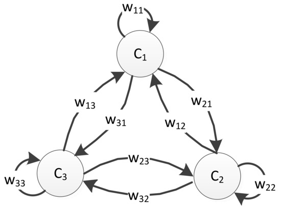
Figure 1.
The framework of a fuzzy cognitive map including three concepts.
Given an FCM including concepts. The activation state values and the weight matrix are expressed as
with being the number of concepts and being the number of samples. The elements in each row of the matrix are the state values of concepts at the corresponding time. The primary mission for constructing an FCM focuses on learning the weight matrix.
The reasoning process of the FCM is generally described as following,
where is the state value of th concept at time , is the state value of th concept at time . In this equation, is the fuzzy weight which shows the value of the influential intensity from concept to . The activation function is a nonlinear monotonically increasing function which squashes the weighted sum of the concepts’ states into a certain interval. One of the most widely used activation functions is the unipolar sigmoid function as given in following,
where is the shape parameter of the function. The state value of the sigmoid function is affected depending on these parameters.
3. The Learning of Least Square Fuzzy Cognitive Map
Different from traditional learning approaches for FCMs, the fuzzy weight matrix is obtained with the least square method in this study. Compared with the traditional method, learning the FCM with least square method is a one-time solution of the matrix equation rather than multi-iteration stochastic searching. The learning of the FCM least square method is abbreviated to LSFCM.
The activation function is a sigmoid function, let us consider the function,
where is the discrete time, , and is the number of concepts. We have,
. Let , then,
The primitive function is and now we have ; the least square method is used to estimate . The sum of squares to be minimized, the fitness function, is described as follows,
The state values of concepts at the current time moment are described by X, X =; it results in a set of concepts’ state values at the next time moment , and . Then, the fitness function can be written in matrix form,
where is a matrix, is the th column of , is the th column of . Then we can solve the estimated as
The term is the L2-norm of which reduces the collinearity of data, .
Let , then , we obtain the solution,
The vector is one column of weight matrix . We the estimated as,
We can obtain the estimated values of by solving (14); there is no iteration and result obtainable at one stroke.
Note that the values of the may not be all in the interval , when the least square method is used to learn the FCM. Owing to , (14) can be rewritten as follows,
It is shown from the formulas that the values of are linearly proportional to the shape parameter , viz., . Suppose , then ; it is not sure that the values of elements of the matrix are all in the interval . In order to obtain the suitable estimated weight matrix, let and , then can be calculated by (15) and the values of elements of the matrix are all in the interval . Algorithm 1 explains the procedure of the LSFCM.
| Algorithm 1: LSFCM |
| Input: Concepts and its state values matrix . |
| 1 X = ; |
| 2 ; |
| 3 If Then |
| 4 ; |
| 5 Else If Then |
| 6 ; |
| 7 End If |
| 8 ; |
| 9 ; |
| 10 , where ; |
| Return the estimated weight matrix . |
4. Modeling Time Series Using LSFCM
This section covers how to use the LSFCM to model time series. The entire process of the modeling is outlined in Figure 2. First, the data are normalized and divided into the training set and test set in chronological order. Second, fuzzy time series are constructed from numerical data based on a fuzzy c-means clustering algorithm. Third, the FCM is learned using the least square method to efficiently obtain the weight matrix of the FCM according to the historical data. After the FCM model is established, we can compute the forecasted values using the LSFCM model.
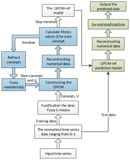
Figure 2.
The outline of proposed method for the time series model.
In order to improve the prediction accuracy of the developed LSFCM model, the model is further optimized by refinement of the concepts. The evolutionary optimization algorithm serves as the optimization vehicle to refine the concepts which have been developed by the fuzzy c-means clustering. The degree of fuzzy membership of each datum to the clusters will be altered and the ensuing LSFCM process is carried out again. The optimization process is driven by the minimization of the reconstruction error. Through these measures, the quality of the FCM model improves. The optimization procedure which is called LSFCM-ref is an iterative process and is repeated until the desired number of iterations is reached. In what follows, the proposed model of forecasting time series will be presented in detail.
4.1. Constructing the LSFCM Model
In this section, the scheme of the proposed time series modeling and prediction approach based on LSFCM and fuzzy c-means clustering is detailed.
When we attempt to model time series with FCMs, the numeric time series should be mapped to a fuzzy time series first. Suppose that the FCM has c concepts and is a numeric time series, then one numerical datum is mapped to a fuzzy set which has c elements in the domain, i.e., , where is the matrix of the concepts and is the fuzzy membership degree of the corresponding to concepts. Then the numeric datum can be present in the fuzzy set form,
Let the given time series normalize to [0,1]. The normalized time series is redefined as . The time series is divided into the training set and test set. The training set containing the datum is used to establish the FCM model; the test set containing the datum is used to estimate the models.
In order to fuzzify the time series, a fuzzy c-means clustering algorithm is used to obtain clustering centers and the fuzzy memberships, the number of the cluster center c is predefined, and the clustering centers are taken as the concepts. We have the concepts’ vectors and the corresponding fuzzy membership matrix . Then the fuzzy membership matrix is used to construct the FCM. There is an internal fuzzy logical relationship between the neighbors of the partition matrix U, viz. . Accordingly, we have n − 1 input–output data pairs, as shown,
Referring to (4), the fuzzy logical relationship between and can be described as follows,
The formula can be expressed in vector form,
According to the LSFCM construction process, the concepts and the fuzzy membership matrix are used as raw material to construct FCM and the least square method is used to learn the FCM. According to Algorithm 1, the weight matrix can be calculated by the following equation,
where and . The elements of the weight matrix can be restricted to the given interval by adjusting the values of . After the processes above, we can obtain a fuzzy cognitive map model of the given time series.
Any datum belonging to the time series can be transformed into the form of fuzzy membership values by the fuzzy c-means algorithm. When the structure of the LSFCM is formed, the dynamic characteristics of the given time series can be interpreted or predicted by the LSFCM. We can predict future fuzzy membership values based on the LSFCM model. According to (19), the forecast membership value , then the forecast datum, can be reconstructed as the following,
where is the concept of FCM, which is calculated by the fuzzy c-means clustering algorithm.
For the quantitative evaluation of LSFCM model quality, the performance index root mean squared error (RMSE) is defined by the following,
where is the number of time series data, is the actual value and is the predictive value of time series at the time t. Obviously, the smaller the RMSE is, the higher the quality of the model is.
4.2. Refinements of LSFCM Model
The concepts of the LSFCM are obtained by the fuzzy c-means algorithm; however the performance index is prediction error. The initial concepts do not necessarily lead to the minimum prediction error. Thus, the idea is to optimize the LSFCM model by adjusting the position of the concepts (cluster centers) for a better performance index. The partition matrix includes the fuzzy membership of each sample to the concepts. Supposing that the position of the concepts is relocated in the domain of definition, on this basis, there will be acting in response to cause a new partition matrix. The structure of the LSFCM will be relearned based on the new partition matrix and concepts, then that impacts directly on the prediction error. The procedure of migration of concepts is depicted in Figure 3. The initial/updated population of concepts is used to construct the LSFCM model. Then, the reconstruction errors are calculated and the optimal concept whose LSFCM model has minimum errors is selected. The best concept is output after the iteration, which is used to construct the optimal LSFCM model. The refinements of concepts will be detailed discussed in the following.
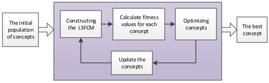
Figure 3.
Migration of concepts.
How to change the position of concepts plays a pivotal role in the process. In this study, the stochastic seeking strategy is considered to adjust the coordinate of all the concepts. It can be believed that the clustering centers of the fuzzy c-means algorithm are already close to the best concepts of the FCM but still make further progress. The position of the clustering center is in the neighborhood of the optimum position which makes the LSFCM model show a better performance index. To refine the FCM model, the initial concepts obtained by fuzzy c-means are used as the starting point. To modify the concepts, a sub-defined interval is introduced for the coordinates of the concepts. The radius of the sub-defined interval is described as follows,
Each concept moves to a new position from its current position in a particular range rather than the entire domain and the new position . Hence, the efficiency of adjustment is higher. The probability of a new concept position in the domain is a normal distribution. In other words, the closer the position to the initial concept, the higher the probability selected. The strategy of concept adjustment is illustrated in Figure 4. The initial population of concepts is a normal distribution. is the probability density function that the position in the domain selects as the new concept. Each concept can move to the best position around the initial position. Although the movement of each concept in each coordinate is random, the movement of all concepts has a preference or tendency. The final result is to minimize the performance index RMSE, viz. .
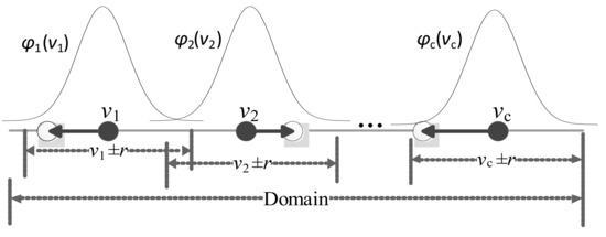
Figure 4.
The strategy of concept adjustment.
The positions of the concepts are adjusted by the evolutionary algorithm Particle swarm optimization (PSO). The fuzzy membership matrix is refreshed corresponding to the new concepts. Once the optimal concepts are obtained, the final LSFCM model (LSFCM-ref) is formed.
5. Results
In this section, publicly available real-world time series are used to demonstrate the effectiveness of the proposed method. All FCM learning methods used for comparative purposes were tested under the same conditions. As previously described, the FCM model is governed mainly by the number of concepts. The shape parameter λ of the sigmoid function also has effect on the performance of the FCM model. In order to evaluate the quality of the proposed methods, there were two purposes of these experiments involving the time series. The first one was that the quantitative evaluation of the impact on the prediction accuracy of the proposed approach being brought by the number of concepts c and the parameter of the sigmoid function. The second one was comparison with other FCM learning methods and the classical forecasting models.
For all the time series, the normalized time series data were split into two samples: training set and test set. The fuzzification coefficient was set to two. There eight time series data sets are applied to evaluate and analyze the developed LSFCM and LSFCM-ref model of time series. The eight time series are given in Table 1 and plotted in Figure 5. In each time series, the first 80% of data were used for model training, the last 20% of data were left for testing purposes.

Table 1.
Experimental data.
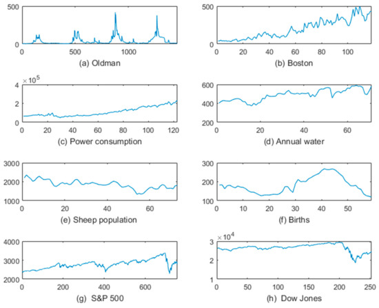
Figure 5.
The experimental data. Different from the number of which directly affects the precision of the least square fuzzy cognitive map (LSFCM) model, the values of do not have an apparent effect for the precision of the LSFCM model, but a large one for the weight matrix. The weight matrix varies linearly inversely with the shape parameter of sigmoid function . The results of the numerical experiments illustrate that various values of represent different , but models with same performance are obtained. For the numerical example of the Births time series (f), the changes with are as follows.
5.1. The Influence of the Parameters of the Proposed Model
The number of the concepts is highly sensitive to the performance of FCM models [35]. The parameters and are particular discussed in the experiments. Optimal values of the parameters are established by inspecting the predictive error (RMSE) of the training set. The values of range from 2, 3,..., 20, while several representative values of are selected. Figure 6 plots line chart groups of RMSE of corresponding different parameter values. Examination of the data shown in Figure 6 leads us to the conclusion that the value of RMSE becomes substantially lower when increasing the number of concepts; however, the value becomes slightly higher or even higher still when the number of concepts exceeds a certain number. In other words, the predictive accuracy does not continuous increase with the increasing number of . For example, regarding the Oldman time series, the optimal value of is 10. Whereas for the Annual water time series, once the number of moves past eight, there will be no substantial improvement of the reconstruction error, or it will become even worse. The topology of the FCM is more complex with the growth of the number of concepts. Therefore, the optimal value of is selected under comprehensive consideration of the topological complexity of the FCM and the predictive accuracy.
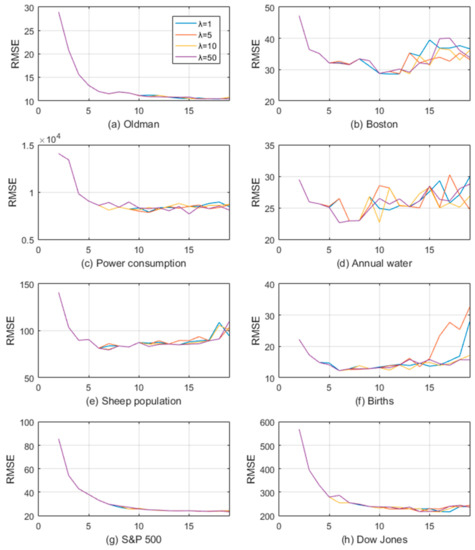
Figure 6.
The performance of the fuzzy cognitive map (FCM) model with different parameters.
Letting , we can calculate the weight matrix,
Then, letting , we have the weight matrix conforming to the definition
If setting , we can also calculate the weight matrix
5.2. Comparison with Other Methods
For comparison, a subset of classical forecasting models was selected for comparison included the Naive, Standard Exponential Smoothing (SES), Holt–Winters and ARIMA models. The details are described in the following sections. The prediction accuracy of the conventional FCMs models was calculated. The prediction accuracy was calculated and listed in Table 2. As can be seen from Table 2, the prediction precision of the time series with FCM learning by the Particle swarm optimization (PSO) or Genetic algorithm (GA) methods is slightly higher than the developed LSFCM prediction model, but less than the LSFCM-ref model. There are no significant differences for all the time series in these models: PSO-FCM, GA-FCM and LSFCM. However, the results with LSFCM-ref model are more accurate than others.
Table 2.
Comparison with other FCM models.
With refinement of concepts, we can further improve the accuracy of the LSFCM model. The comparison shows that the developed FCM prediction model can produce satisfactory quality for the time series. It can be seen in Figure 7 that the location of the concepts changes with refinements. In the coordinates, the black star points are the initial position of the concepts, and the red circles are the final position of optimized concepts.
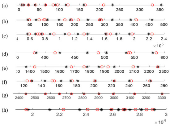
Figure 7.
Adjustment concepts. Black star points: the initial position, red circles: the final position.
Furthermore, the comparison between the proposed approach and the classical prediction approach (Naive, SES, Holt–Winters and ARIMA) is presented in Table 3. As can be noted, the LSFCM approach outperformed the classical prediction models and the LSFCM has the minimum RMSE compared with the other prediction methods.
Table 3.
Comparison with the classic prediction models.
6. Conclusions
A novel FCM learning approach for time series was proposed in this study. The model contains two stages. The first one is to construct an FCM model with the least square method, viz. LSFCM. The second one is to optimize the LSFCM with refinement of concepts to improve the prediction accuracy. Fuzzy c-means clustering is applied to fuzzify the given time series data set to automatically extract the FCM’s concepts and fuzzy membership matrix. Two important contributions of the proposed method are learning the FCM with the least square method and refinement of concepts. The former can help the FCM learning eliminate the strenuous iterative computation. The latter can help the FCM obtain the optimal concepts by relocating the position of concepts. In addition, the stochastic strategy is applied to refine the concepts of the LSFCM. The influence of the parameters of the FCM on the prediction accuracy is analyzed. The number of concepts significantly impacts the prediction accuracy of the LSFCM prediction model. When the number of clusters is assigned to the optimal value, the ideal numerical prediction accuracy can be obtained. The parameters of activation function have no great effect on the prediction accuracy of the LSFCM model but have a big impact on the weight matrix. From the results of experimentation, LSFCM is a very competitive model for time series modeling and forecasting.
Author Contributions
Conceptualization, G.F.; formal analysis, G.F.; investigation, G.F. and W.L.; methodology, G.F. and J.Y.; supervision, J.Y.; validation, G.F., W.L. and J.Y. All authors have read and agreed to the published version of the manuscript.
Funding
This research received no external funding.
Conflicts of Interest
The authors declare no conflict of interest.
References
- Yardimci, A. Soft computing in medicine. Appl. Soft Comput. 2009, 9, 1029–1043. [Google Scholar] [CrossRef]
- Song, Q.; Chissom, B.S. Fuzzy time series and its models. Fuzzy Sets Syst. 1993, 54, 269–277. [Google Scholar] [CrossRef]
- Singh, P. A brief review of modeling approaches based on fuzzy time series. Int. J. Mach. Learn. Cybern. 2015, 8, 397–420. [Google Scholar] [CrossRef]
- Bose, M.; Mali, K. Designing fuzzy time series forecasting models: A survey. Int. J. Approx. Reason. 2019, 111, 78–99. [Google Scholar] [CrossRef]
- Kosko, B. Fuzzy cognitive maps. Int. J. Man Mach. Stud. 1986, 24, 65–75. [Google Scholar] [CrossRef]
- Felix, G.; Nápoles, G.; Falcon, R.; Froelich, W.; Vanhoof, K.; Bello, R. A review on methods and software for fuzzy cognitive maps. Artif. Intell. Rev. 2019, 52, 1707–1737. [Google Scholar] [CrossRef]
- Froelich, W.; Salmeron, J.L. Evolutionary learning of fuzzy grey cognitive map for the forecasting of multivariate, interval-valued time series. Int. J. Approx. Reason. 2014, 55, 1319–1335. [Google Scholar] [CrossRef]
- Nápoles, G.; Grau, I.; Papageorgiou, E.; Bello, R.; Vanhoof, K. Rough Cognitive Networks. Knowl. Based Syst. 2016, 91, 46–61. [Google Scholar] [CrossRef]
- Salmeron, J.L.; Vidal, R.; Mena, A.; Mena-Nieto, A. Ranking fuzzy cognitive map based scenarios with TOPSIS. Expert Syst. Appl. 2012, 39, 2443–2450. [Google Scholar] [CrossRef]
- Stach, W.; Kurgan, L.; Pedrycz, W. A divide and conquer method for learning large Fuzzy Cognitive Maps. Fuzzy Sets Syst. 2010, 161, 2515–2532. [Google Scholar] [CrossRef]
- Stach, W.; Kurgan, L.; Pedrycz, W. A Survey of Fuzzy Cognitive Map Learning Methods. Available online: http://128.172.132.65/papers/chapterSurveyFCM2003.pdf (accessed on 20 January 2021).
- Papageorgiou, E.I. Learning Algorithms for Fuzzy Cognitive Maps—A Review Study. IEEE Trans. Syst. Man Cybern. Part C Appl. Rev. 2012, 42, 150–163. [Google Scholar] [CrossRef]
- Papageorgiou, E.; Stylios, C.; Groumpos, P. Fuzzy Cognitive Map Learning Based on Nonlinear Hebbian Rule. In Australasian Joint Conference on Artificial Intelligence; Springer International Publishing: Berlin/Heidelberg, Germany, 2003; pp. 256–268. [Google Scholar]
- Papageorgiou, E.I.; Stylios, C.D.; Groumpos, P.P. Active Hebbian learning algorithm to train fuzzy cognitive maps. Int. J. Approx. Reason. 2004, 37, 219–249. [Google Scholar] [CrossRef]
- Papageorgiou, E.I.; Groumpos, P. A weight adaptation method for fine-tuning Fuzzy Cognitive Map causal links. Soft Comput. 2005, 9, 846–857. [Google Scholar] [CrossRef]
- Stach, W.; Kurgan, L.; Pedrycz, W.; Reformat, M. Genetic learning of fuzzy cognitive maps. Fuzzy Sets Syst. 2008, 153, 371–401. [Google Scholar] [CrossRef]
- Ghazanfari, M.; Alizadeh, S.; Fathian, M.; Koulouriotis, D.E. Comparing simulated annealing and genetic algorithm in learning FCM. Ap-pl. Math. Comput. 2007, 192, 56–68. [Google Scholar] [CrossRef]
- Papageorgiou, E.I.; Parsopoulos, K.E.; Stylios, C.S.; Groumpos, P.P.; Vrahatis, M.N. Fuzzy Cognitive Maps Learning Using Particle Swarm Optimization. J. Intell. Inf. Syst. 2005, 25, 95–121. [Google Scholar] [CrossRef]
- Mateou, N.H.; Moiseos, M.; Andreou, A.S. Multi-objective evolutionary fuzzy cognitive maps for decision support. In Proceedings of the IEEE Congress on Evolutionary Computation, CEC 2005, Edinburgh, UK, 2–4 September 2005; pp. 824–830. [Google Scholar]
- Froelich, W.; Juszczuk, P. Predictive Capabilities of Adaptive and Evolutionary Fuzzy Cognitive Maps—A Comparative Study. In Intelligent Systems for Knowledge Management; Springer: Berlin/Heidelberg, Germany, 2009; pp. 153–174. [Google Scholar]
- Wu, K.; Liu, J. Learning of Sparse Fuzzy Cognitive Maps Using Evolutionary Algorithm with Lasso Initialization. In Asia-Pacific Conference on Simulated Evolution and Learning; Springer: Cham, Switzerland, 2017; pp. 385–396. [Google Scholar]
- Lu, W.; Feng, G.; Liu, X.; Pedrycz, W.; Zhang, L.; Yang, J. Fast and Effective Learning for Fuzzy Cognitive Maps: A Method Based on Solving Constrained Convex Optimization Problems. IEEE Trans. Fuzzy Syst. 2020, 28, 2958–2971. [Google Scholar] [CrossRef]
- Feng, G.; Lu, W.; Pedrycz, W.; Yang, J.; Liu, X. The Learning of Fuzzy Cognitive Maps with Noisy Data: A Rapid and Robust Learning Method with Maximum Entropy. IEEE Trans. Cybern. 2019, 1–13. [Google Scholar] [CrossRef]
- Stach, W.; Kurgan, L.A.; Pedrycz, W. Numerical and Linguistic Prediction of Time Series with the Use of Fuzzy Cognitive Maps. IEEE Trans. Fuzzy Syst. 2008, 16, 61–72. [Google Scholar] [CrossRef]
- Papageorgiou, E.I.; Froelich, W. Application of Evolutionary Fuzzy Cognitive Maps for Prediction of Pulmonary Infections. IEEE Trans. Inf. Technol. Biomed. 2011, 16, 143–149. [Google Scholar] [CrossRef]
- Papageorgiou, E.I.; Froelich, W. Multi-step prediction of pulmonary infection with the use of evolutionary fuzzy cognitive maps. Neurocomputing 2012, 92, 28–35. [Google Scholar] [CrossRef]
- Yang, S.; Liu, J. Time-Series Forecasting Based on High-Order Fuzzy Cognitive Maps and Wavelet Transform. IEEE Trans. Fuzzy Syst. 2018, 26, 3391–3402. [Google Scholar] [CrossRef]
- Lu, W.; Yang, J.; Liu, X.; Pedrycz, W. The modeling and prediction of time series based on synergy of high-order fuzzy cognitive map and fuzzy c-means clustering. Knowl. Based Syst. 2014, 70, 242–255. [Google Scholar] [CrossRef]
- Lu, W. The Hybrids Algorithm Based on Fuzzy Cognitive Map for Fuzzy Time Series Prediction. J. Inf. Comput. Sci. 2014, 11, 357–366. [Google Scholar] [CrossRef]
- Homenda, W.; Jastrzębska, A.; Pedrycz, W. Nodes Selection Criteria for Fuzzy Cognitive Maps Designed to Model Time Series. In Intelligent Systems’ 2014; Springer: Cham, Switzerland, 2015; Volume 323, pp. 859–870. [Google Scholar]
- Salmeron, J.L.; Froelich, W. Dynamic optimization of fuzzy cognitive maps for timeseries forecasting. Knowl. Based Syst. 2016, 105, 29–37. [Google Scholar] [CrossRef]
- Froelich, W.; Papageorgiou, E.I.; Samarinas, M.; Skriapas, K. Application of evolutionary fuzzy cognitive maps to the long-term prediction of prostate cancer. Appl. Soft Comput. 2012, 12, 3810–3817. [Google Scholar] [CrossRef]
- Homenda, W.; Jastrzebska, A.; Pedrycz, W. Modeling time series with fuzzy cognitive maps. In Proceedings of the 2014 IEEE International Conference on Fuzzy Systems (FUZZ-IEEE), Beijing, China, 6–11 July 2014; pp. 2055–2062. [Google Scholar]
- Bezdek, J.C.; Ehrlich, R.; Full, W. FCM: The fuzzy c-means clustering algorithm. Comput. Geosci. 1984, 10, 191–203. [Google Scholar] [CrossRef]
- Pedrycz, W.; Jastrzebska, A.; Homenda, W. Design of fuzzy cognitive maps for modeling time series. IEEE Trans. Fuzzy Syst. 2016, 24, 120–130. [Google Scholar] [CrossRef]


Publisher’s Note: MDPI stays neutral with regard to jurisdictional claims in published maps and institutional affiliations. |
© 2021 by the authors. Licensee MDPI, Basel, Switzerland. This article is an open access article distributed under the terms and conditions of the Creative Commons Attribution (CC BY) license (http://creativecommons.org/licenses/by/4.0/).