Application of Mini-Batch Metaheuristic Algorithms in Problems of Optimization of Deterministic Systems with Incomplete Information about the State Vector ^†

Abstract

In this paper, we consider the application of the zero-order mini-batch optimization method in the problem of finding optimal control of a pencil of trajectories of nonlinear deterministic systems in the case of incomplete information about the state vector. The pencil of trajectories originates from a given set of initial states. To solve the problem, the structure of a feedback system is proposed, which contains models of the plant, measuring system, nonlinear state observer and control law of the fixed structure with unknown coefficients. The objective function proposed considers the quality of pencil of trajectories control, which is estimated by the average value of the Bolz functional over the given set of initial states. Unknown control laws of a plant and an observer are found in the form of expansions in terms of orthonormal systems of basis functions, which are specified on the set of possible states of a dynamical system. The original pencil of trajectories control problem is reduced to a global optimization problem, which is solved using the well-proven zero-order method, which uses a modified mini-batch approach in a random search procedure with adaptation. An algorithm for solving the problem is proposed. The satellite stabilization problem with incomplete information is solved.

1. Introduction

A general approach to the numerical solution of the problem of finding the average optimal control of nonlinear deterministic dynamical systems under conditions of uncertainty in setting the initial conditions and incomplete information about the state vector is proposed. Since direct information about the state vector is not available, a nonlinear state observer is included in the closed-loop control system, which finds an estimate of the state vector from the output of the nonlinear model of the measuring system. The control laws of the plant and the observer are found simultaneously as functions of time and estimates of the state vector. In contrast to linear systems with a quadratic criterion, in which the synthesis of the optimal controller and the optimal filter is performed independently, in the proposed procedure, the undefined coefficients of the control laws of the plant and the observer are sought simultaneously [1].

An alternative way is to use various numerical methods for solving the Bellman equation as a sufficient condition for optimality of feedback control in the complete state information problem. In this case, arbitrary initial conditions are considered, for which the minimum of the functional should be obtained. When solving practical problems of control theory, it is usually possible to define a set of initial states, determined by the conditions of operation of the control system, and for this set to search for the corresponding law of control with feedback. To complete the solution, one should find the parameters of the nonlinear observer independently and use the estimate of the state vector in the optimal control law instead of exact information about the state vector.

In the present paper, the behavior of a nonlinear continuous deterministic plant (model of object) is described by the ODE system. Parallelepiped constraints are imposed on control vector coordinates. Initial conditions are given by a compact set of initial states. The quality of separate trajectory control is estimated by the value of the Bolz functional. For the given set of initial conditions, a pencil of trajectories is considered. The performance index to be minimized is calculated by the average value of the Bolz functional over the set of initial states. The problem is to find the control laws for the plant and the state observer in the class of functional expansions in terms of elements of orthonormal basis systems with unknown coefficients, depending on time and estimates of the state vector coordinates. The components of the control laws are found using systems of basis functions that are used in problems of spectral analysis [2,3]. It is proposed to apply the mini-batch adaptive method of random search (MAMRS) [4,5,6] for solving the problem under consideration and to analyze the solution of the problem for various models of the measuring system. As a special case, the control problem with complete information about the state vector is considered. MAMRS can be classified as a metaheuristic method [7,8,9,10,11]. MAMRS extends the idea of stochastic gradient methods [12,13,14,15] to a method that does not require information about the gradient. The efficiency and analysis of this method is demonstrated by solving an applied optimal control problem of satellite stabilization [16].

2. Statement of the Problem

We consider the nonlinear continuous dynamical system described by the vector differential equation:

$$\dot{x}(t)=f(t,x(t),u(t)),$$

(1)

where $f(t,x,u)$ is a given continuous function, $t\in T=[t_0;t_1]$ is a continuous time and the initial moment $t_0$ and final moment $t_1$ are specified; $x\in R^n$ is a state vector; $u\in U\subseteq R^q$ is a control vector and $U=[a_1,b_1]\times \dots \times [a_q,b_q]$ is a set of allowable values of control.

The initial conditions are specified as:

$$x(t_0)=x_0\in \Omega \subset R^n,$$

(2)

where Ω is a set with positive measure ($\mathrm{mes}\hspace{0.17em}\Omega >0$) and a piecewise smooth boundary. It characterizes the uncertainty in setting the initial conditions.

The model of the measuring system is described by the relation:

$$z(t)=h\left(t,x(t)\right),$$

(3)

where $z\in R^m$ is an output vector and $h\left(t,x\right)$ is a given continuous function. The information coming from the model of the measuring system arrives at the input of the state observer, producing an estimate of the state vector.

We suppose that it is possible to obtain an estimate of the state vector using a nonlinear observer of the form:

$$\frac{d\widehat{x}(t)}{dt}=f\left(t,\widehat{x}(t),u(t,\widehat{x}(t))\right)+K(t,\widehat{x}(t))[z(t)-h(t,\widehat{x}(t))],$$

(4)

$$\widehat{x}(t_0)={\widehat{x}}_0,$$

(5)

where $\widehat{x}(t)$ is a state vector estimate, ${\widehat{x}}_0\in \Omega$ is an initial estimate and $K(t,\widehat{x})\in R^{n\times m}$ is an unknown continuous $n\times m$ matrix function. This matrix is considered as a feedback control of the observation process. The state vector estimate is used also in the plant control law $u(t,\widehat{x})$.

We define the set of admissible control laws $\mathbf{U}$ by functions $(u(t,\widehat{x}),K(t,\widehat{x}))$, where $\forall t\in T$, the plant control $u(t)=u(t,{\widehat{x}}^{}(t))\in U$ is a piecewise continuous and the observer control $K(t)=K(t,\widehat{x}(t))\in R^{n\times m}$ is a continuous function. It is assumed that the solution of the system of Equations (1) and (4) with the initial conditions (2), (5) taking into account (3), exists and is unique.

The performance index for a separate trajectory:

$$I\left(x_0,u(t,\widehat{x}(t)),K(t,\widehat{x}(t))\right)={\displaystyle \underset{t_0}{\overset{t_1}{\int }}{f}^0\left(t,x(t),u(t,\widehat{x}(t)),K(t,\widehat{x}(t))\right)}dt+F\left(x(t_1)\right),$$

(6)

where $f^0(t,x,u,K),F(x)$ are given continuous functions.

We associate the pencil of trajectories of the system of Equations (1) and (4) with each admissible control law $(u(t,\widehat{x}),K(t,\widehat{x}))\in \mathbf{U}$ and the set $\Omega$ of initial states:

$$X\left(t,u(t,\widehat{x}),K(t,\widehat{x})\right)=\cup \left\{x\left(t,u(t,\widehat{x}),K(t,\widehat{x}),x_0\right),\widehat{x}\left(t,\mathrm{U}(t,\widehat{x}),K(t,\widehat{x}),{\widehat{x}}_0\right)|x_0\in \Omega \right\},$$

that is, the union of the system of Equations (1) and (4) and solutions for all possible initial states from the set $\Omega$.

The performance index for the pencil of trajectories control to be minimized is:

$$J\left[\mathrm{U}(t,\widehat{x}),K(t,\widehat{x})\right]={\displaystyle \underset{\Omega }{\int }I\left(x_0,\mathrm{U}(t,\widehat{x}(t)),K(t,\widehat{x}(t))\right)}d{x}_0/\mathrm{mes}\hspace{0.17em}\Omega \hspace{0.17em}.$$

(7)

The optimal control problem is to choose the control policy $(u*(t,\widehat{x}),K*(t,\widehat{x}))\in \mathbf{U}$ so that performance index (7) is minimized:

$$J\left[{\mathrm{U}}^{*}(t,\widehat{x}),K^{*}(t,\widehat{x})\right]=\underset{(u\left(t,\widehat{x}\right),K(t,\widehat{x}))\in u}{\min \hspace{0.17em}}J\left[u(t,\widehat{x}),K(t,\widehat{x})\right]$$

(8)

Since the average value of performance index (6) is minimized on the set of initial states $\Omega$, the required control is called optimal on average.

3. Solution Search Strategy

We consider the transition to the parametric optimization problem from the control problem (8), i.e., to the problem of finding unknown coefficients of the plant control and the observer control. The plant control constraints of parallelepiped type should be taken into account.

To implement this transition, we use the following assumptions:

1.

The set of initial states $\Omega$ is a parallelepiped, defined by the direct product of segments $\left[{\alpha }_i;{\beta }_i\right],i=\overline{1,n},$ i.e., $\Omega =\left[{\alpha }_1;{\beta }_1\right]\times \cdots \times \left[{\alpha }_n;{\beta }_n\right]$. With the help of a step $\Delta x_i$, all line segments are divided into $N_i$ segments and the parallelepiped $\Omega$ is divided into $N=N_1\cdots N_n$ elementary disjoint subsets ${\Omega }_k,\hspace{0.17em}k=\overline{1,N}$. In each elementary subset ${\Omega }_k$, an initial state $x_0{}^k$ (the center of the parallelepiped ${\Omega }_k$ is specified;

2.

The direct product $Q=[\underset{\_}{x_1},\overline{x_1}]\times \cdots \times [\underset{\_}{x_n},\overline{x_n}]$ represents the set of admissible values of the state vector coordinates, where $\underset{\_}{x_i},\overline{x_i},\hspace{0.17em}\hspace{0.17em}i=\overline{1,n}$ are the lower and upper boundaries for each coordinate, respectively, determined by the applied problem being solved. Therefore, one can assume that the possible estimates of the state vector should satisfy the following conditions: ${\widehat{x}}_1\in [\underset{\_}{x_1},\overline{x_1}],\dots ,{\widehat{x}}_n\in [\underset{\_}{x_n},\overline{x_n}]$;

3.

The plant control policy is searched in the form:

$$u_j\left(t,\widehat{x}(t)\right)=\mathrm{sat}\underset{v_j(t)}{\underbrace{\left\{g_j\left(t,{\widehat{x}}_1(t),\dots ,{\widehat{x}}_n(t)\right)\right\}}},\hspace{0.17em}j=\overline{1,q},$$

(9)

where saturation function sat guarantees the fulfillment of the plant control constraints of the form $a_j\le u_j(t)=u_j(t,\widehat{x}(t))\le b_j$:

$$\mathrm{sat}\hspace{0.17em}{v}_j(t)=\{\begin{array}{l}{v}_j(t),\hspace{0.17em}\hspace{0.17em}\hspace{0.17em}\hspace{0.17em}{a}_j<v_j(t)<b_j,\\ a_j,\hspace{0.17em}\hspace{0.17em}\hspace{0.17em}\hspace{0.17em}{v}_j(t)\le a_j,\\ b_j,\hspace{0.17em}\hspace{0.17em}\hspace{0.17em}\hspace{0.17em}{v}_j(t)\ge b_j,\end{array}$$

(10)

$$g_j\left(t,{\widehat{x}}_1,\dots ,{\widehat{x}}_n\right)={\displaystyle \sum _{i_0=0}^{L_0-1}{\displaystyle \sum _{i_1=0}^{L_1-1}\cdots {\displaystyle \sum _{i_n=0}^{L_n-1}{u}_{i_0,i_1,\dots ,i_n}^j\cdot q\left(i_0,t\right)p_1(i_1,{\widehat{x}}_1)\cdots p_n\left(i_n,{\widehat{x}}_n\right)},}}$$

(11)

where $u_{i_0,i_1,\dots ,i_n}^j$ are unknown coefficients; $L_0,L_1,\dots ,L_n$ are scales of truncation; $q\left(i_0,t\right),i_0=\overline{0,L_0-1}$ is a system of orthonormal time functions (basis functions) defined on the segment $[t_0,t_1]$ and satisfying the condition ${\displaystyle \underset{t_0}{\overset{t_1}{\int }}q(i,t)q(j,t)dt=\{\begin{array}{c}1,i=j,\\ 0,i\ne j,\end{array}}$; and $p_j(i_j,{\widehat{x}}_j),i_j=\overline{0,L_j-1}$ is a system of orthonormal functions of a variable ${\widehat{x}}_j$ (basis functions) defined on an interval $[\underset{\_}{x_j},\overline{x_j}]$, $j=1,\dots ,n$.

As the basis functions $q\left(i_0,t\right),\hspace{0.17em}{p}_k\left(i_k,{\widehat{x}}_k\right),\hspace{0.17em}k=\overline{1,n}$, one can take, for example:

• Legendre polynomials:

$$p\left(n,x\right)={\displaystyle \sum _{k=0}^n{\left(C_n^k\right)}^2{\tilde{x}}^{n-k}}\hspace{0.17em}{\tilde{x}}^k,\hspace{0.17em}n=\overline{0,L-1};$$

• Cosine:

$$p\left(n,x\right)=\cos \left(n\cdot \pi \cdot (2\cdot \tilde{x}-1)\right),n=\overline{0,L-1};$$

where $\tilde{x}=(x-\underset{\_}{x})/(\overline{x}-\underset{\_}{x})$ and other systems of basic functions.

The matrix entries $K_{ij}(t,\widehat{x}),i=1,\dots ,n;j=1,\dots ,m$ of the state observer control policy $K(t,\widehat{x})$ are found by a formula similar to (11), where variable $u$ is replaced by $K$.

The value of the pencil control cost functional (7) is approximated as:

$$J\left[u\left(t,\widehat{x}\right),\hspace{0.17em}K\left(t,\widehat{x}\right)\right]\cong (1/N){\displaystyle \sum _{k=1}^{N}I\left(x_0,u(t,\widehat{x}(t)),K(t,\widehat{x}(t))\right)}.$$

(12)

The optimization problem is to choose the best parameters $u_{i_0,i_1,\dots ,i_n}^j$, $K_{i_0,i_1,\dots ,i_n}^{i,j}$, minimizing performance index (12) by using a mini-batch adaptive method of random search (MAMRS) [4]. The strategy of its application is that, for the approximate calculation of functional (12), randomly selected $d$ non-coinciding trajectories emanating from the set of initial states are used that form a mini-batch:

$$J_d\left[u\left(t,\widehat{x}\right),\hspace{0.17em}K\left(t,\widehat{x}\right)\right]=(1/d){\displaystyle \sum _{k=1}^{d}I\left(x_0,u(t,\widehat{x}(t)),K(t,\widehat{x}(t))\right)}.$$

(13)

The mini-batch size is user-definable,$1\le d\le N$, and is usually selected step by step. Furthermore, for simplicity of presentation, we assume that each coordinate of the control laws $u(t,\widehat{x})$ and $K(t,\widehat{x})$ can be associated with a matrix column of the coefficients $u_{i_0,i_1,\dots ,i_n}^j$, $K_{i_0,i_1,\dots ,i_n}^{i,j}$. Furthermore, by concatenation, one can represent the entire set of optimized parameters in the form of an extended vector. Let us denote it by $K_d$ and assume that it has dimension $(n\times 1)$. The objective function is denoted by $J_d(K_d)$. For each mini-batch size $1\le d\le N$, the optimization results are different. When $d\to N$, the accuracy of solving the optimization problem in general increases.

4. Mini-Batch Adaptive Search Algorithm

Let us consider the optimization problem $J_d[K_d]\to \underset{K_d}{\min }$.

Denote: $J_d^s$ is the minimum value of the cost function after the $s-$th run; ${\widehat{K}}_d^s$ is a best parameter vector column after startup; $d$ is the mini-batch size.

Step 0. Set the initial mini-batch size: $d=1$ (in general, one can start with any value of $1\le d\le N$); $S_{\max }$ is a maximum number of starts; $B_{\max }$ is a maximum number of passes; $\alpha =1.618$ is an expansion coefficient; $\beta =0.618$ is a compression coefficient; M is a maximum number of failed tests at the current iteration; $t_0=1$ is an initial step size (one can use any value $t_0>R$), R is a minimum step size and L is a maximum number of iterations; and $r$ is a number of initial trial solutions ($1\le r\le 10$).

Step 1. Set the values:$b=1$ (passes number counter) and $P_d=0$(initial value of the sum of the cost function average values).

Step 2. Set the values: $s=1$(starts number counter) and $J_d^1={10}^8÷{10}^{10}$; $S_d=0$(initial value of the sum of the objective function values).

Step 3. Define the initial values of coefficients $u_{i_0,i_1,\dots ,i_n}^j$,$k_{i_0,i_1,\dots ,i_s}^{ij}$. Generate r vectors $K_d^s$ using a uniform distribution of its coordinates at some intervals. Calculate the value of the function $J_d$ for each generated vector and order them according to the value of the objective function [17]. The vector with the smallest value of the objective function is denoted by column vector $K_d^s{}^{,0}$. Put $l=0,j=1$.

Step 4. Generate a random vector ${\xi }^j={\left({\xi }_1{}^j,\dots ,{\xi }_{qn}{}^j\right)}^T$, where ${\xi }_i{}^j$ is a random variable uniformly distributed on the interval [−1,1].

Step 5. Calculate: $y^j=K_d^s{}^{,l}+t_l\frac{{\xi }^j}{\Vert \hspace{0.17em}{\xi }^j\hspace{0.17em}\Vert }$.

Step 6. Generate the mini-batch size $d$, i.e., generate $d$ pairwise mismatched sets of $q_1\in N_1,\dots ,q_n\in N_n$ values defining the initial states $X_0^k\in \Omega$ with numbers $k=q_1\cdot \dots \cdot q_n\in \{1,\dots ,N\}$ or corresponding to the tuple $<q_1,\dots ,q_n>$.

Check the fulfillment of the conditions:

(a)

If $J_d(y^j)<J_d(K_d^s{}^{,l})$, the algorithm step is successful. Put $z^j=K_d^{s,l}+\mathsf{\alpha }(y^j-K_d^{s,l})$. Determine if current direction $y^j-K_d^s{}^{,l}$ is successful: if $J_d(z^j)<J_d(K_d^s{}^{,l})$, the search direction is successful. Put $K_d^s{}^{,l+1}=z^j$, t_l+1 = αt_l, l = l + 1 and check the termination condition. If l < L, put j = 1 and go to step 4. If l = L, the search process is over: ${\widehat{K}}_d^s=K_d^s{}^{,l}$, go to step 8; if $J_d(z^j)\ge J_d(K_d^s{}^{,l})$, the search direction is unsuccessful, go to step 7;

(b)

If $J_d(y^j)\ge J_d(K_d^s{}^{,l})$, the unsuccessful step is made, go to step 7.

Step 7. Calculate the number of unsuccessful steps from the current solution:

(a)

If j < M, put j = j + 1 and go to step 4;

(b)

If j = M, check the termination condition: if $t_l\le R$, the process is over: ${\widehat{K}}_d^s=K_d^s{}^{,l}$ and $J_d^s=J_d(K_d^s{}^{,l})$, go to step 8; if $t_l>R$, put t_l = β t_l, j = 1 and go to step 4.

Step 8. Check the improvement of the cost function value as a result of the $s$-th run: if $J_d(K_d^s{}^{,l})<J_d^s$, put $J_d^s=J_d(K_d^s{}^{,l})$ and ${\widehat{K}}_d^s=K_d^s{}^{,l}$ and go to step 9; if $J_d(K_d^s{}^{,l})\ge J_d^s$, go to step 9.

Step 9. Calculate $S_d=S_d+J_d^s$ and verify the stop conditions (the maximum number of starts is achieved): if $s<S_{\max }$, put $s=s+1$ and go to step 3; if $s=S_{\max }$, put ${\widehat{K}}_d={\widehat{K}}_d^s$—the best solution during the $b$-th pass for a given $d$; calculate $m_d=S_d^s/S_{\max }$ and ${\sigma }_{m_d}={\left(\frac{1}{S_{\max }-1}{{\displaystyle \sum _{s=1}^{S_{\max }}\left[J_d^s-m_d\hspace{0.17em}\right]}}^2\right)}^{1/2}$ and go to step 10.

Step 10*. Put $P_d=P_d+m_d$ and $m_d^b=m_d$ and check the condition for completing a given number of passes: if $b<B_{\max }$, put $b=b+1$ and go to step 2; if $b=B_{\max }$,calculate: ${\overline{m}}_d={\displaystyle \sum _{b=1}^{B_{\max }}{m}_d^b}/B_{\max }$, ${\sigma }_{{\overline{m}}_d}={\left(\frac{1}{B_{\max }-1}{{\displaystyle \sum _{b=1}^{B_{\max }}\left[m_d^b-{\overline{m}}_d\hspace{0.17em}\right]}}^2\right)}^{1/2}$.

Step 11*. Check the condition for completing studies of the effect of the mini-batch size: if $d<N$, put $d=d+1,s=1$ and go to step 1; if $d=N$, go to step 12.

Step 12. As a result, find the best estimate of ${\widehat{K}}_d^{*}$ after $B_{\max }$ passes and indicators ${\overline{m}}_d$ and ${\sigma }_{{\overline{m}}_d}$ for each value of the mini-batch size $d$. To analyze the resulting estimation accuracy, find the value $J({\widehat{K}}_d^{*})$.

Steps 10 and 11 are performed if necessary. It is recommended to do restarts to increase the chances of finding a global extremum. The best solution is selected from the restarts made.

5. Satellite Stabilization Problem

The problem of damping the rotational motion of the satellite by the engines installed on it is considered. The system describing the motion of a rigid body relative to the center of inertia after the transition to dimensionless variables has the form:

$$\{\begin{array}{l}\dot{p}(t)=[u_1(t)/6],\\ \\ \dot{q}(t)=[u_2(t)-0.2r(t)\hspace{0.17em}p(t)],\\ \\ \dot{r}(t)=[0.2\hspace{0.17em}\hspace{0.17em}\left(u_3(t)+p(t)\hspace{0.17em}q(t)\right)],\end{array}$$

where $p,q,r$ are the projections of the angular velocity onto the main central axes of inertia and $t\in [0,1]$ and $u_1,u_2,u_3$ are controls that characterize the thrust of the engines located on the satellite.

The set of initial states is given by a uniform distribution law on the set $\Omega =[23;25]\times [13;15]\times [13;15].$

At the final moment of the system functioning, the following conditions must be fulfilled: $p(1)=q(1)=r(1)=0,$ corresponding to the meaning of the satellite stabilization problem. The fulfillment of terminal conditions should be accompanied by minimization of the fuel used to turn the satellite.

The functional (6):

$$I={\displaystyle \underset{0}{\overset{1}{\int }}[\hspace{0.17em}\left|u_1(t)\right|+\left|u_2(t)\right|+\left|u_3(t)\right|]\hspace{0.17em}dt}+{10}^3\cdot [p^2(1)+q^2(1)+r^2(1)].$$

Next, we will consider two examples: the joint estimations and control problem with incomplete information about the state vector and the optimal control problem with complete information about the state vector.

5.1. Example 1. The Joint Estimation and Control Problem

The proposed observer equation is:

$$\{\begin{array}{l}\frac{d\widehat{p}}{dt}=u_1(t,\widehat{x}(t))/6+K_1(t,\widehat{x}(t))[z(t)-h(t,\widehat{x}(t))],\\ \\ \frac{d\widehat{q}}{dt}=u_2(t,\widehat{x}(t))-0.2\hspace{0.17em}\widehat{r}\hspace{0.17em}\widehat{p}+K_2(t,\widehat{x}(t))[z(t)-h(t,\widehat{x}(t))],\\ \\ \frac{d\widehat{r}}{dt}=0.2\hspace{0.17em}\hspace{0.17em}\left(u_3(t,\widehat{x}(t))+\widehat{p}\hspace{0.17em}\widehat{q}\right)+K_3(t,\widehat{x}(t))[z(t)-h(t,\widehat{x}(t))].\end{array}$$

Further, we will consider the cases of solving the problem with different models of the measuring system.

In all tests, the number of initial states is $\hspace{0.17em}N=27$ and $L_0=L_1=L_2=L_3=2$ is the scale of truncation. The initial state estimation vector is $\widehat{x}(0)={\widehat{x}}_0={(24,15,13)}^T$. Parameters of the mini-batch adaptive method of random search are $B_{\max }=1000$, $M=15$ and $R=8\cdot {10}^{-5}$. To synthesize the plant control $u(t,\widehat{x})$ and observer control $K(t,\widehat{x})$, a system of orthonormal Legendre polynomials is used.

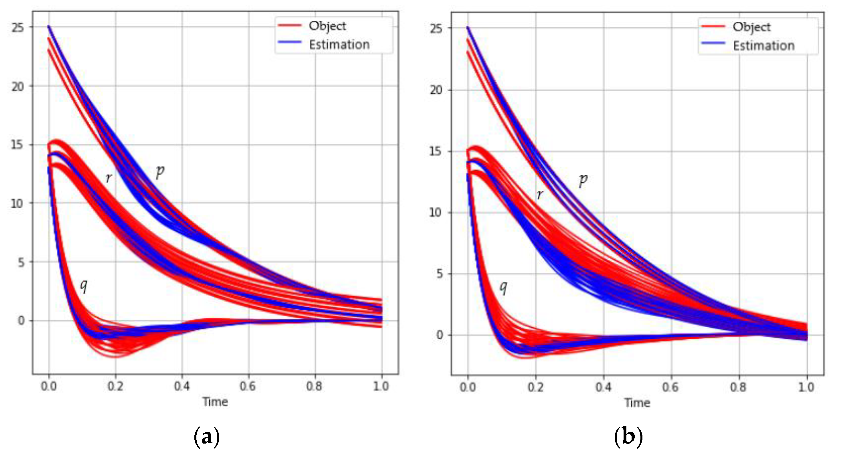
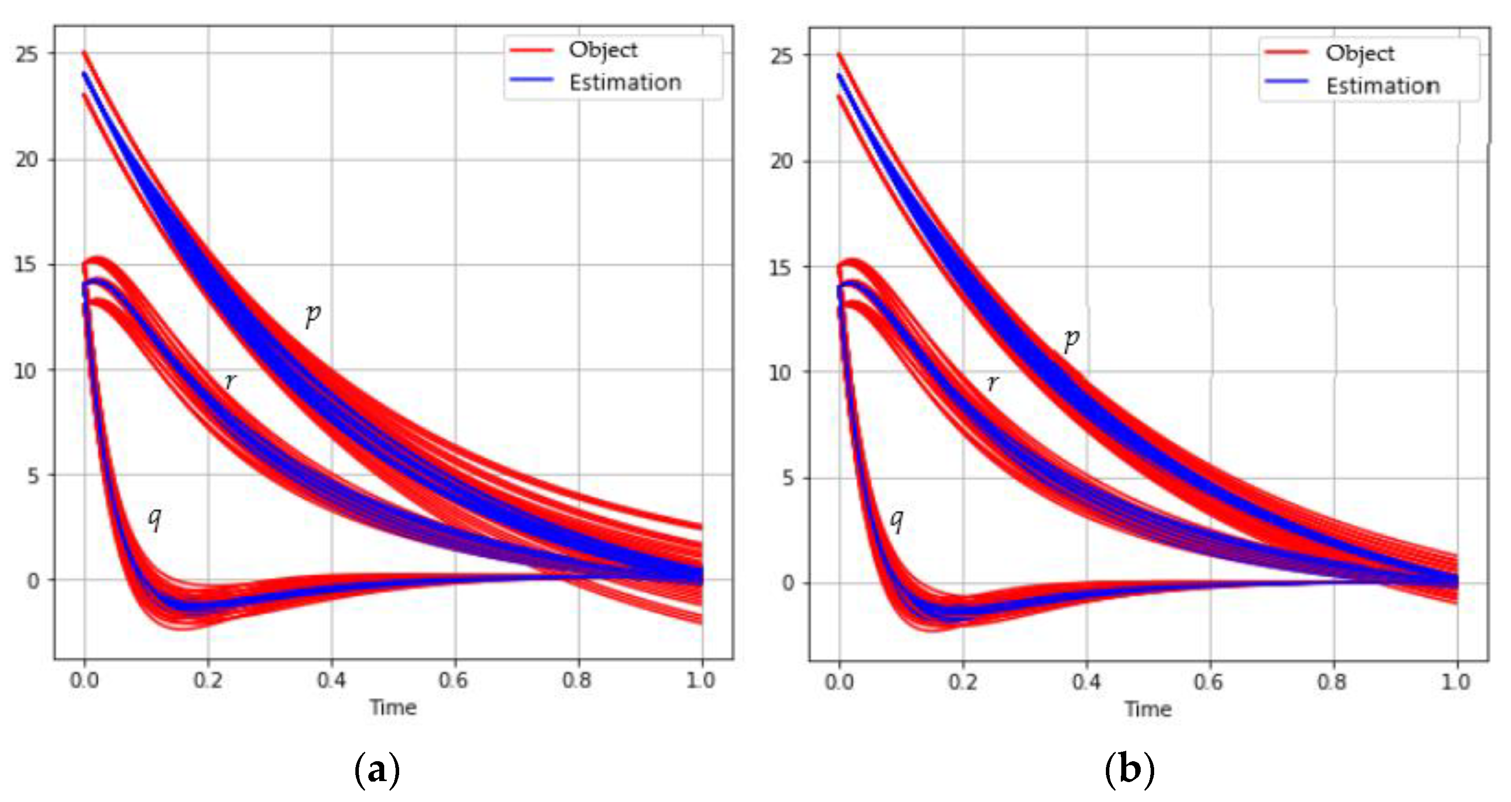
5.1.1. Case A

The measuring system model is described by the following relationship:

$$z(t)={\left(r(t),p(t)\right)}^{\mathrm{T}}$$

The behavior of trajectories set for different mini-batch sizes is shown in Figure 1:

Table 1. Solution results for different mini-batch sizes.

$\mathit{d}$	$\mathit{J}[{\mathit{K}}_{\mathit{d}}]$
1	2970.9487
10	315.6251
20	256.9266
27	167.1622

shows the results of solving the problem depending on the mini-batch size.

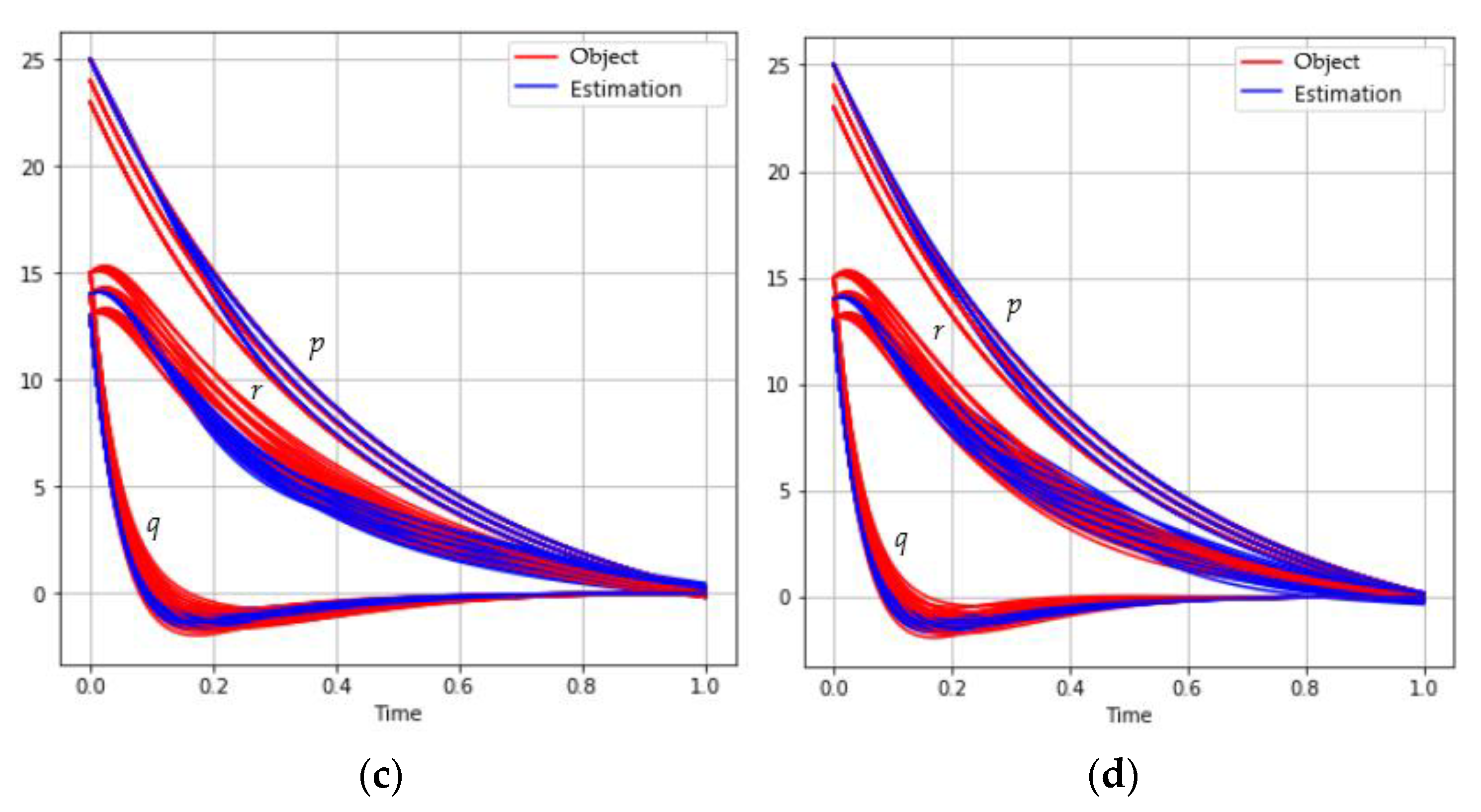
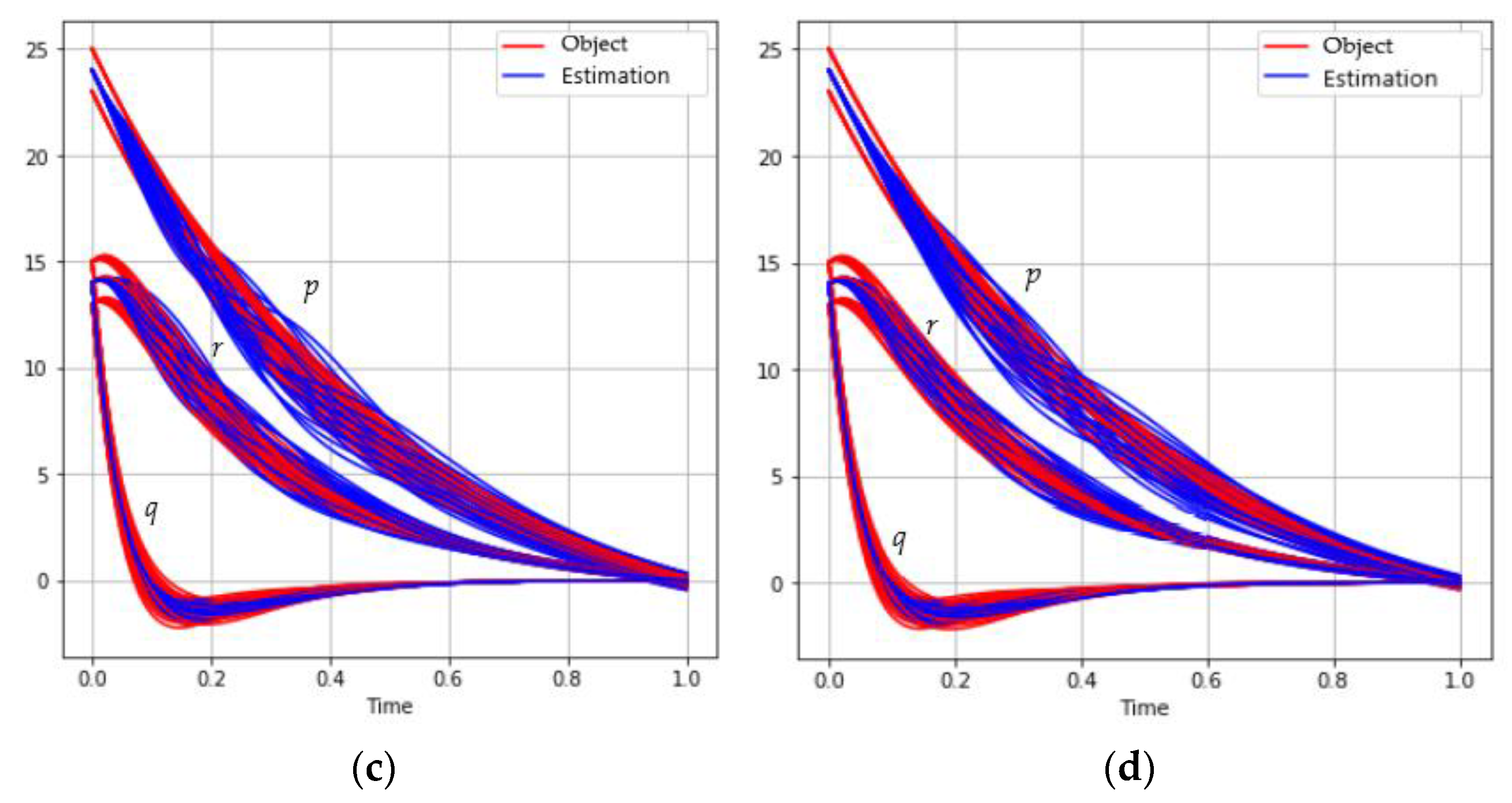
5.1.2. Case B

The measuring system model is described by the following relationship:

$$z(t)={(p(t),q(t))}^{\mathrm{T}}$$

The behavior of the trajectories set for different sizes of mini-batch is shown in Figure 2:

Table 2. Solution results for different mini-batch sizes.

$\mathit{d}$	$\mathit{J}[{\mathit{K}}_{\mathit{d}}]$
1	2722.1031
10	455.5253
20	311.6676
27	236.1635

shows the results of solving the problem depending on the mini-batch size.

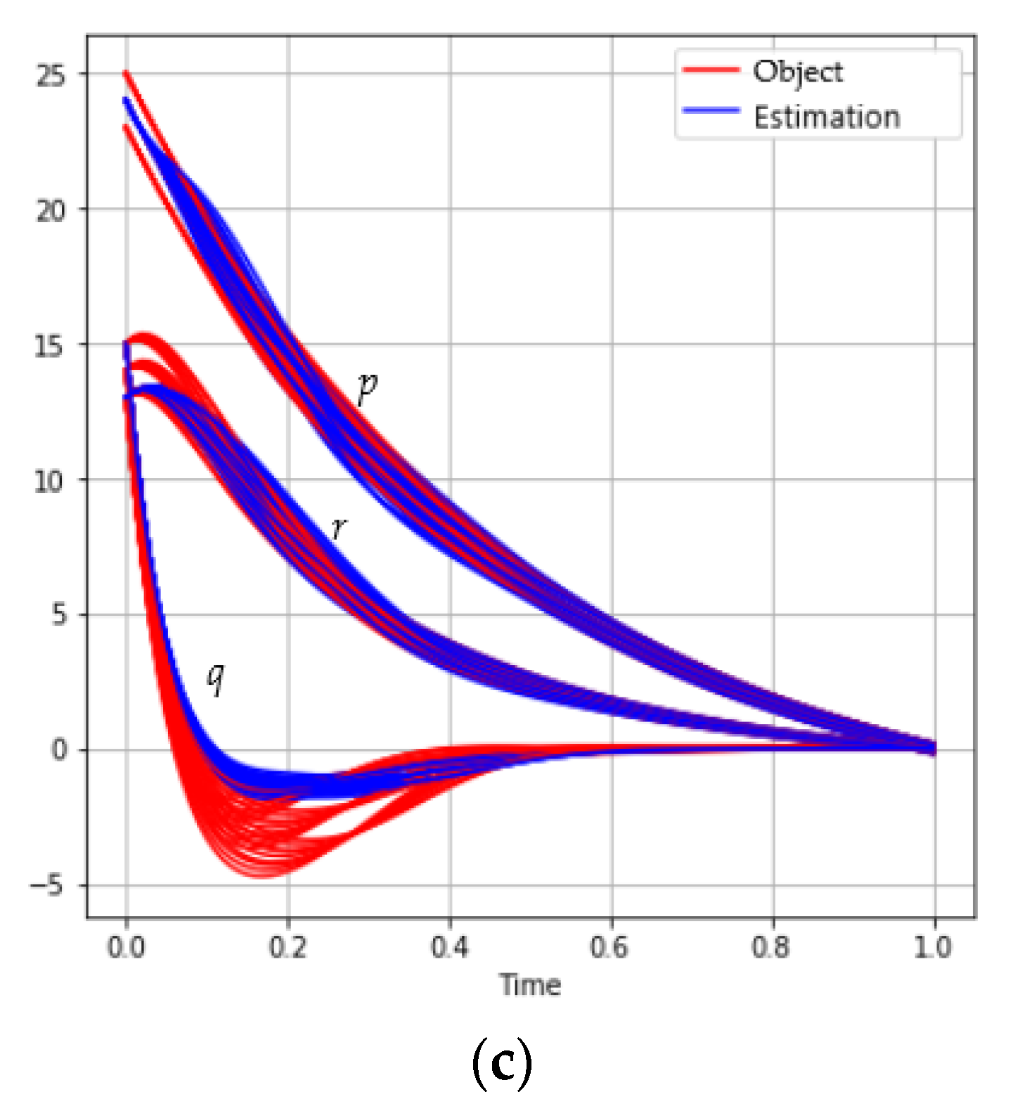
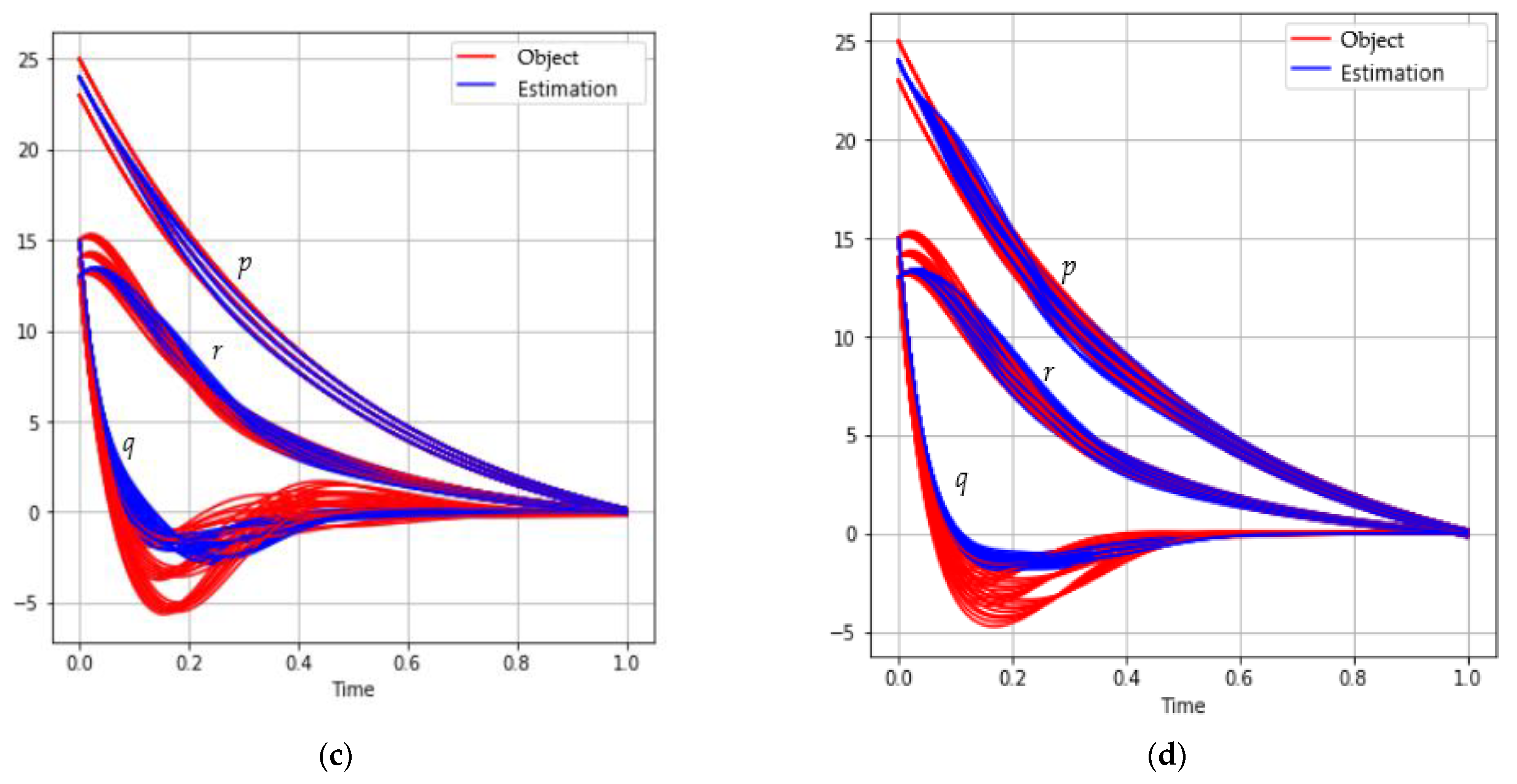
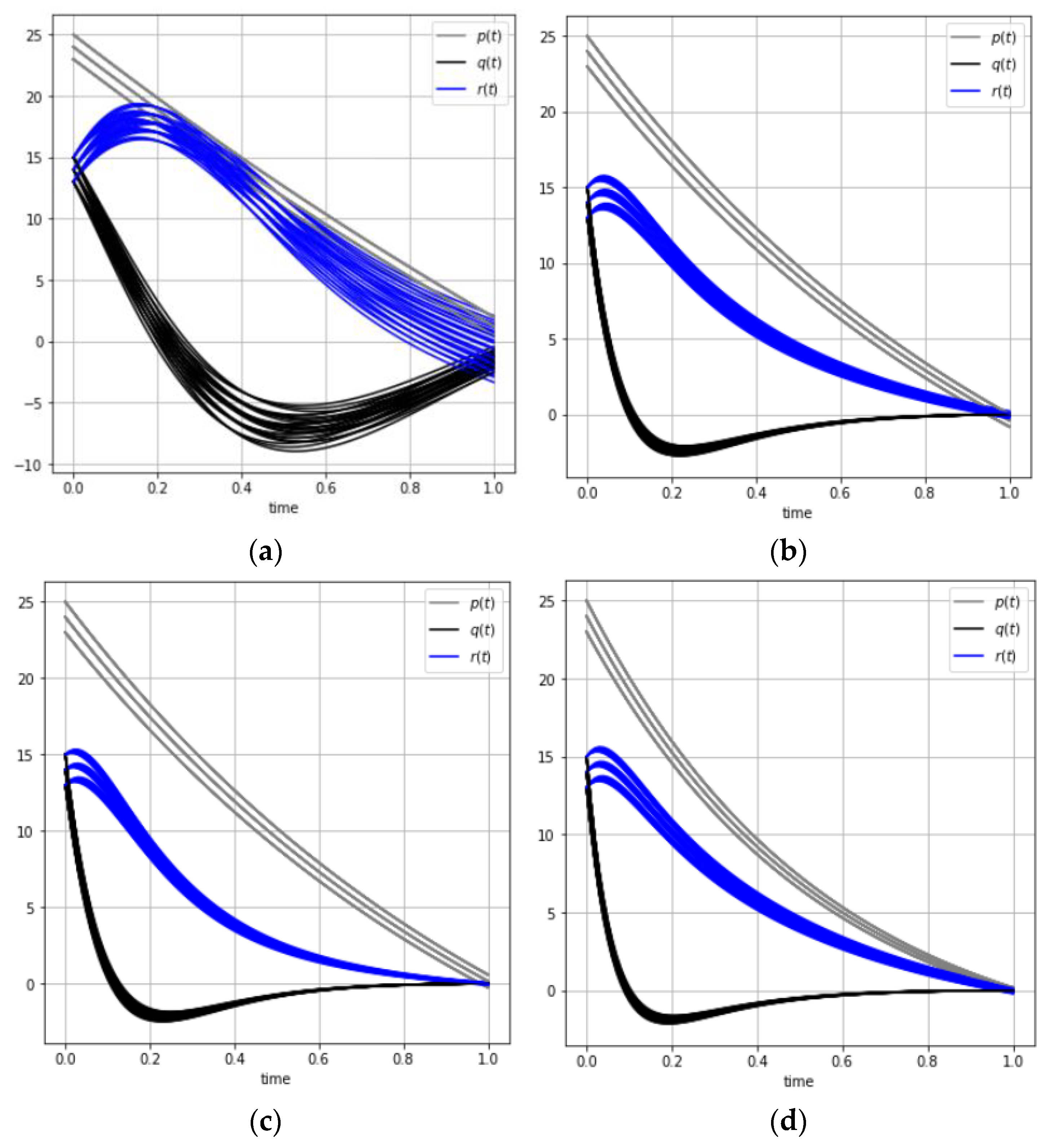
5.1.3. Case C

The measuring system model is described by the following relationship:

$$z(t)={(r(t),q(t))}^{\mathrm{T}}$$

The behavior of the trajectories set for different sizes of mini-batch is shown in Figure 3:

Table 3. Solution results for different mini-batch sizes.

$\mathit{d}$	$\mathit{J}[{\mathit{K}}_{\mathit{d}}]$
1	2934.4927
10	860.9751
20	405.3041
27	351.7748

shows the results of solving the problem depending on the mini-batch size.

Based on Table 1, Table 2 and Table 3, we can conclude that, with an increase of the mini-batch size, the accuracy of the problem solution also increases.

Figure 4 and

Table 4. Solution results for different mini-batch sizes.

$\mathit{d}$	$\mathit{z}(\mathit{t})$	$\mathit{J}[{\mathit{K}}_{\mathit{d}}]$
27	${(r(t),q(t))}^{\mathrm{T}}$	351.7748
27	${(p(t),q(t))}^{\mathrm{T}}$	236.1635
27	${(r(t),p(t))}^{\mathrm{T}}$	167.1622

show the solution to the problem of satellite stabilization depending on the selected model of measuring systems with a mini-batch $d=27$:

From Figure 4 and Table 4, a similar character of convergence for different models of the measuring system is observed.

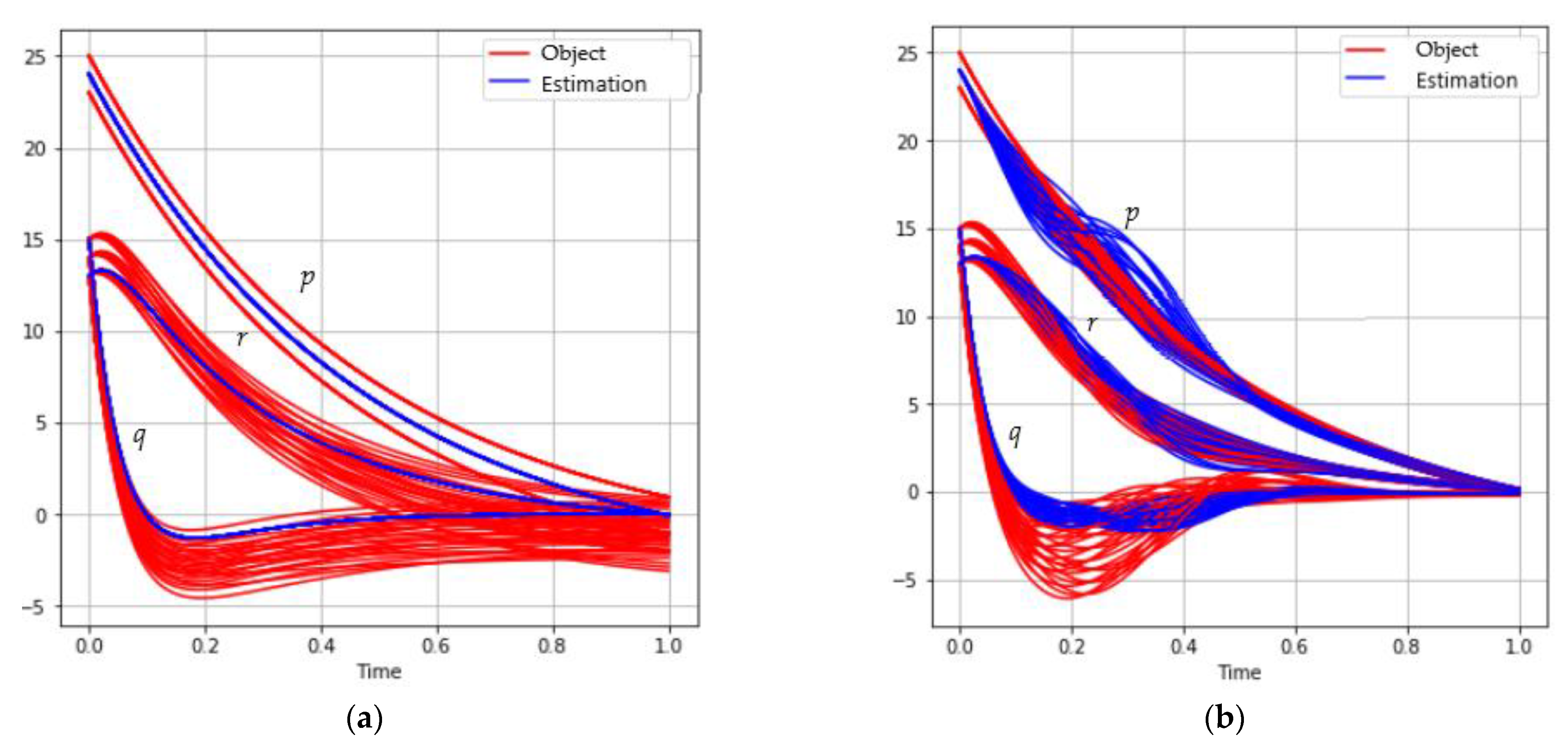
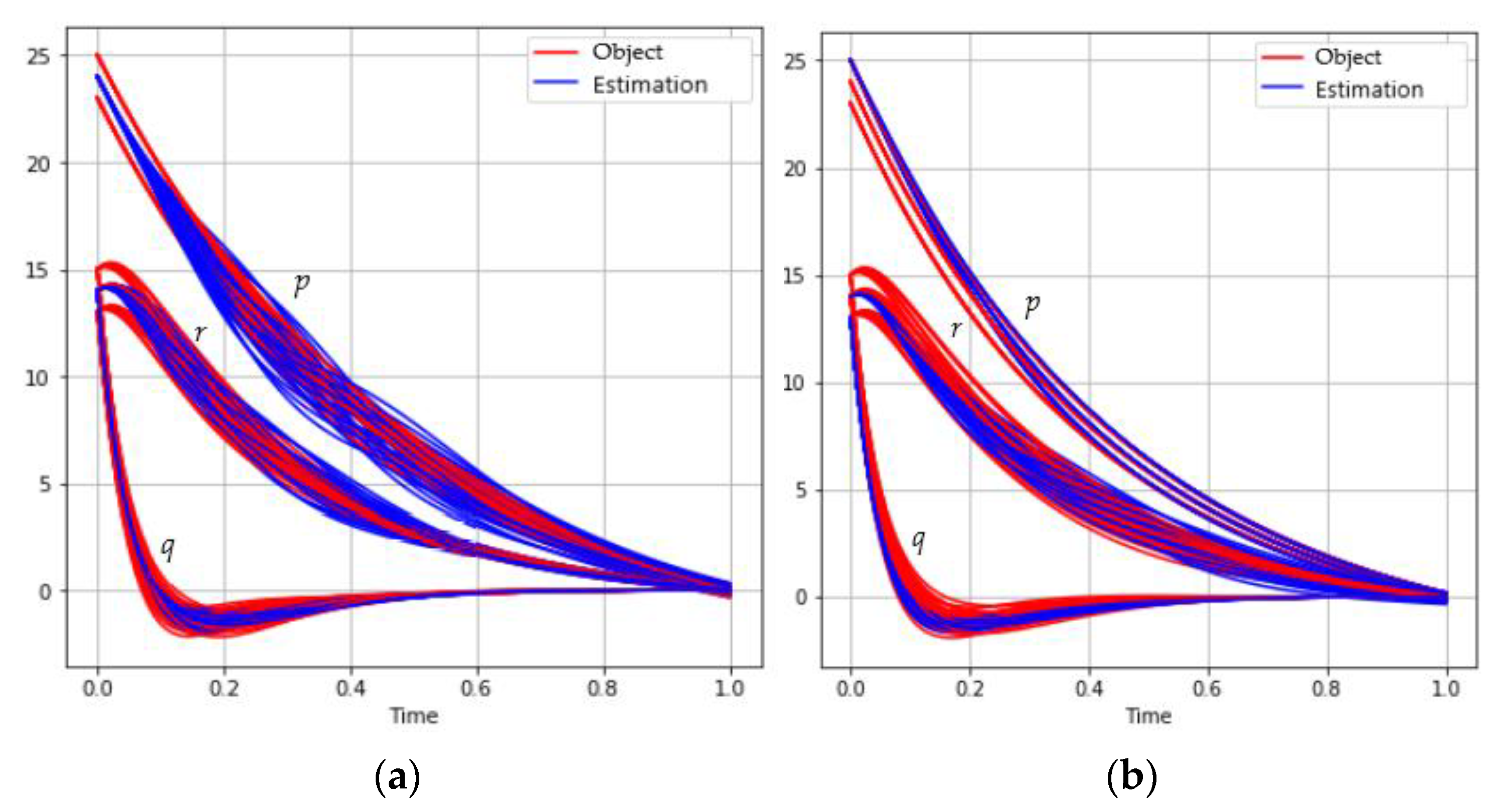
5.2. Example 2. The Control Problem with Complete Information about the State Vector

The measuring system model is described by the following relationship:

$$z(t)={(p(t),q(t),r(t))}^{\mathrm{T}}$$

In this case, there is no need to use a state observer because there is complete information about the state vector at an arbitrary moment in time. In practice, this case is rarely realized, but it is of interest for the analysis of losses in terms of the value of the cost functional associated with the incompleteness of the information received. In all tests, the number of generated random initial states is $N=27$ and $L_1=L_2=L_3=2$ is the scale of truncation. Parameters of the mini-batch adaptive method of random search are $B_{\max }=1000$, $M=30$ and $R=8\cdot {10}^{-9}$. To synthesize the plant control $u(t,x)$, a system of orthonormal Legendre polynomials is used.

The behavior of trajectories set for different sizes of mini-batch is shown in Figure 5:

Table 5. Solution results for different mini-batch sizes.

$\mathit{d}$	$\mathit{J}[{\mathit{K}}_{\mathit{d}}]$
1	1129.1925
10	217.4981
20	196.9630
27	98.8108

shows the results of solving the problem depending on the mini-batch size.

Based on the results of examples 1 and 2, we can conclude that, with the mini-batch size $d=10$, good convergence of the estimates of the state vector coordinates to the true values is already achieved. The total execution time of the algorithm with the mini-batch size $d=10$ was 30 min and with the mini-batch size $d=27$ was 90 min based on an INTEL CORE i5 2.10 GHz processor. The results obtained indicate that, when using mini-batches, the required quality of transients is achieved at reasonable computational costs.

6. Conclusions

The developed zero-order metaheuristic optimization algorithm, namely, a mini-batch adaptive method of random search, is tested on the satellite stabilization problem of finding the optimal control for a pencil of trajectories of nonlinear deterministic systems emanating from a given set of initial states. The software for solving the problem of satellite stabilization is developed. Three cases of solving the problem for different models of the measuring system with incomplete information are considered. The analysis of the problem solution for different models of the measuring system with incomplete information is carried out. A comparison is made with the solution of the problem with a model of the measuring system containing complete information about the state vector. The study of the influence of the mini-batch size on the accuracy of the solution in each considered problem is carried out. Recommendations on the choice of the algorithm parameters are given. The obtained numerical results confirm the idea that, for a certain mini-batch size, an acceptable quality of transient processes can be achieved with low computational costs.