1. Introduction
Reinforcement learning, as the main branch of machine learning, has been widely used in the field of control. Due to its strong real-time performance and adaptability, it can reach or even surpass the capability of traditional control algorithms in many fields [
1]. Compared with designing the controller by the traditional learning method, reinforcement learning learns the optimal strategy step by step through the simulation experiment. Its model setting is usually defined as dynamic programming, so it is more suitable for the real-time and dynamic control system. Especially in the face of complex nonlinear real-time systems, such as air traffic control and automatic manufacturing systems, it is difficult for researchers to work out an appropriate control system, which requires the use of a system with online learning ability [
1,
2] for processing.
Reinforcement learning interacts with the environment through agents (control objects), sampling the currently defined environment states and actions in different states. For existing states and state-action pairs, the algorithm evaluates by defining value functions. In other words, the reinforcement learning is a process in which agents interact with the environment to generate actual returns and the state function and action function are iterated continuously to obtain the optimal strategy and maximize the cumulative reward [
1]. Since this process relies on the reinforcer and is similar to the learning process of animals [
3], it is called reinforcement learning.
It has become a mainstream method of reinforcement learning to use a deep neural network [
4,
5] as a value function fitter. With the continuous maturity of network frameworks such as Tensorflow [
6] and Pytorch [
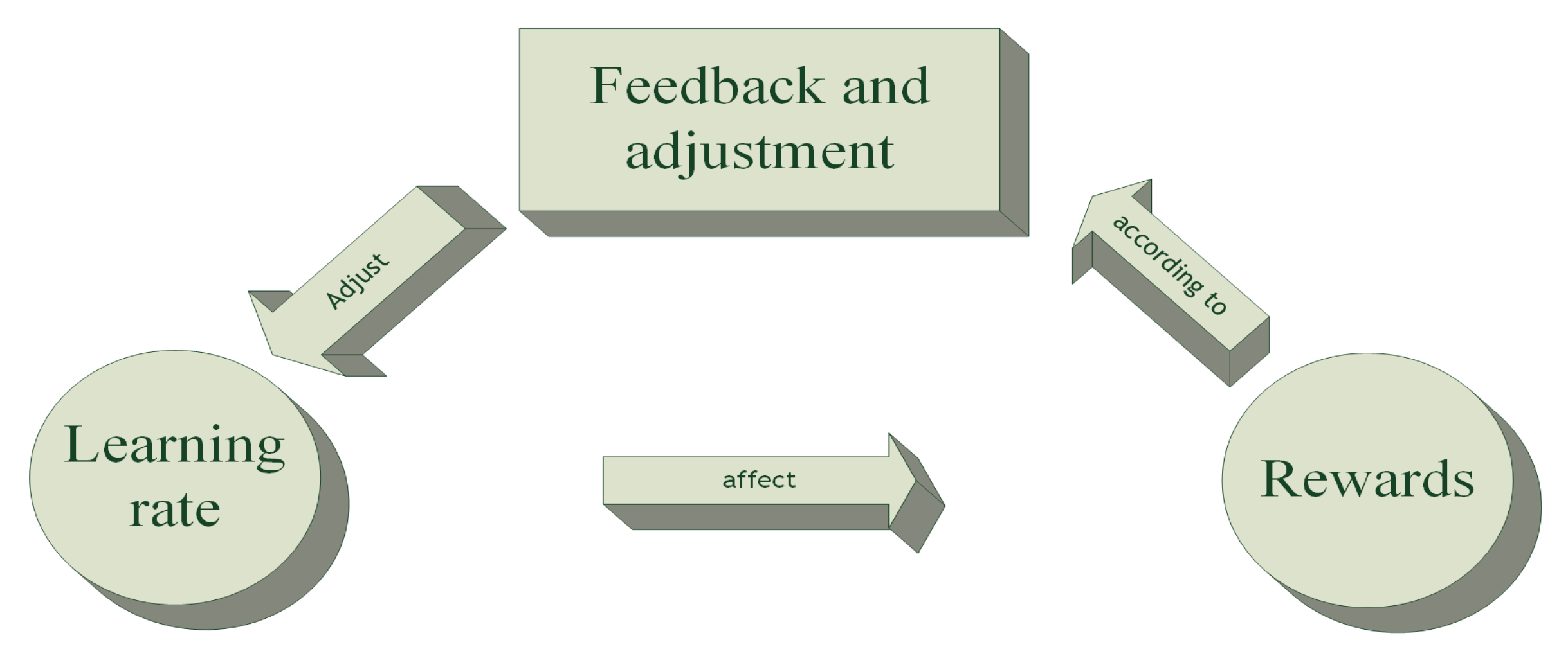
7], network construction has become a fixed process. Network setup and hyperparameter selection have also become process based on experience. The network structure and application of deep reinforcement learning have their particularity. However, the mode of parameter regulation is still the empirical and attempted regulation in the neural network. At present, the parameter setting of an intelligent controller based on reinforcement learning is mostly regulated by empirical setting and result feedback. In this paper, the effect of the learning rate on the performance of deep reinforcement learning algorithm is discussed. In the models of supervised learning and unsupervised learning, we can judge and adjust the learning rate according to the fitting degree of the final objective function. However, in reinforcement learning, the target function is dynamic. Because agents also need to rely on algorithms to explore strategies and further optimize their targets to update network parameters. Therefore, the error of the network update also contains the information of the agent to explore the new strategy. However, at present, we still use similar models of supervised learning and unsupervised learning in the setting of learning rate in the model of realizing deep reinforcement learning, which can be seen in
Figure 1. It will result in the loss of the agent’s information in the search for the optimal strategy and ultimately affect the cumulative return effect of the algorithm. We believe that if we can effectively use this part of the information hidden in the deep reinforcement learning model, then we can optimize the existing model. Because reinforcement learning has dynamic programming characteristics, we think it is unreasonable to use the method similar to supervised learning directly [
8]. More importantly, the network structure of deep reinforcement learning also relies on the learning rate parameter to adjust the stability and exploration ability [
9] of the algorithm. Therefore, we believe that using the same learning rate in different stages is not reasonable for reinforcement learning.
At the same time, the setting of the learning rate is closely related to the stability of the algorithm performance in both supervised learning and unsupervised learning and deep reinforcement learning. Especially in deep reinforcement learning, the adjustment method used now only considers the accumulated rewards, as the feedback signal of parameter adjustment is unreasonable [
10]. Although some learning rates cannot be compared with the current “optimal” learning rate, they have advantages in other performances, such as the learning speed of the algorithm’s early income strategy. Therefore, we consider that if the advantages of different learning rates can be combined, the algorithm may be able to achieve better results than the traditional learning rate method to some extent.
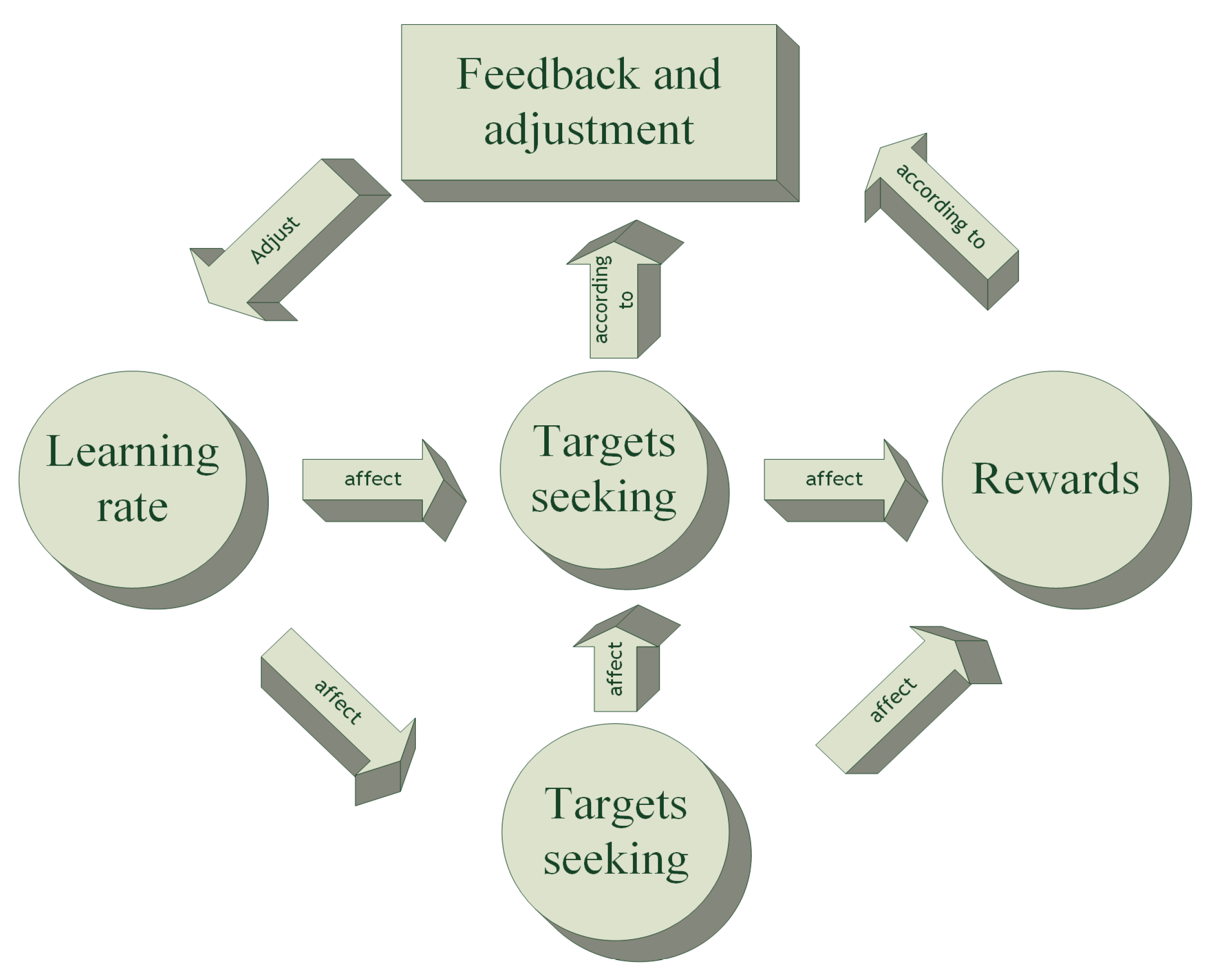
This paper puts forward a parameter setting method of dynamically adjusting the learning rate based on temporal-difference (TD) learning by analyzing the model theory of reinforcement learning. This method has a more setting basis than the traditional setting process of “guessing-adjustment-contrast-adjustment” [
8,
9]. At the same time, this method can use reinforcement learning to explore the potential information in a better strategy and dynamically adjust the learning rate. It can be seen in
Figure 2. Theoretically, we provide the basis for the convergence of the proposed algorithm by combining the Robbins–Monro approximation algorithm [
11]. Then, experiments show that the controller “rationality” of the algorithm is improved. At the same time, we also prove that the results obtained by the proposed algorithm are significantly improved in terms of rationality and convergence. This not only provides a paradigm for setting parameters, but also improves the performance of the algorithm.
Different from traditional reinforcement learning setting parameters, this paper puts forward the vector, dynamically adjusting the train of thought and theoretical basis for the reinforcement learning controller design, and provides a new idea and the basis for a dynamic state vector evaluation that also deserves further research.
The arrangement of this paper is as follows: In
Section 2, we will explain the train of thought and theoretical basis for adjusting the setting of the learning rate. In
Section 3 we will show the results of dynamically adjusting the learning rate. In
Section 4, the process of dynamic adjustment is summarized and the prospect of this method is explored.
2. Temporal-Difference Learning
Different from the turn-based games [
12], the control objects of controllers in practical applications are mostly continuous control rather than turn-based control. Therefore, compared with iterative updating based on the turn-based system, temporal-difference iteration has more advantages [
13]. At the same time, the process of sequential difference iteration is more similar to the dynamic programming process in which people dynamically process and adjust the planning to achieve the task under the limitation of the given goal.
A more intuitive example: Suppose the guest is going to be at home at a certain time, and you need to prepare for it. You have to go to the supermarket, the butcher, and the winery. Based on experience, you know the estimated driving time between all destinations. You think you can complete the shopping in the last two stores in ten minutes. Because of the congestion, you assume it takes 60 min to get to the supermarket. Therefore, you and the guest make an appointment to meet at home at noon. Let us say you get to the supermarket, it takes you 10 min to finish your shopping, and you get home in 20 min. However, on the way from the butcher to the winery, you find the traffic is heavy, so it takes you 30 min to get home. You end up arriving home 10 min later than you had predicted. This example illustrates the dynamic adjustment capability of the TD Learning. After you get the value update between the two steps, you can dynamically adjust the “home time”. This means that existing estimates can be adjusted each time based on existing observations. There is no need to update after the end of the turn along with the actions taken and the value gained.
In theory, TD learning is a bootstrapping method of estimation [
14,
15]. This method has great advantages in dynamic programming. Its model naturally forms beggar’s online, incremental learning. This makes this approach useful not only for turn-based games but also for actual non-turn-based control objects. At the same time, this method does not need to scan the whole state space, but only needs to update the traversed path incrementally.
Q learning [
16,
17] is a typical sequential difference learning algorithm, and it can also seem like a paradigm [
18,
19]. The core of the algorithm is to minimize the gap between the estimated value and the actual value. It can be expressed as a normal Equation (
1):
where
V is a state-valued function.
t is the mark of time.
s represents the observed state
s of the agent at time
t.
stands for the state the agent is likely to move to at the next moment.
r is the timely reward agent recieved when the state
s is transferred to
. The same symbols in the following text have the same meaning.
In fact, most algorithms in TD Learning can be represented by such a normal form. It is just that there is a difference at the core of the algorithm. is the learning rate, and its size determines the learning effect. However, most of the current algorithms cannot provide the setting rules of each parameter of the algorithm. At present, most experiments and environments use empirical methods to test the learning rate of the algorithm. This makes it difficult to ensure that the hyperparameters used in the algorithm can achieve the desired effect or optimal performance. Meanwhile, the learning rate of the algorithm is now only related to the final goal of the controlled object. In other words, the algorithm uses constructional parameters that only guarantee that the computation will accrue more returns.
Indeed, the cumulant of the reward value is a significant factor in evaluating the rationality of the algorithm. However, this way of designing parameters ignores the “convergence” of the algorithm. In our experiment, it is found that different parameters in different stages of training also have a great influence on the convergence of the algorithm. It can be considered that the learning rate of the algorithm affects the cumulative return and convergence performance of the algorithm at the same time. Therefore, we need a reasonable way to decouple their effects and optimize them simultaneously.
Therefore, this paper presents a dynamic adjustment algorithm using a learning rate method. By using a mapping method, the TD loss in reinforcement learning is used as an evaluation index, and the learning rate used by the algorithm is dynamically adjusted during online learning.
3. The Method of Dynamic Adjustment Learning Rate and Convergence Proof
The basic framework of a reinforcement learning is modeled on the Markov Decision Process (MDP) [
20]. This is the basis for our analysis. Quaternions
are commonly used to describe the MDP.
S is a finite set of states for all the actions contained by the
;
A is the limited space of the
’s action; actions are used to control state transitions in the system.
P is defined as
,
R is defined as the reward function
.
is the probability that the Agent will turn from
S to
after performing the action A.
.
represents the rewards that the system gives to the agent after the agent executes action
a and the system changes from state
s to state
. The policy defines the behavior of agents in a given state and determines the actions of agents.
,
is the probability of executing action
a in state
s. In the MDP, it also defines two kinds of value functions (value function): State PI value function
(state value function) and state-action value function
(state-action value function).
represents the expected rewards of the agent according to the strategy starting from state
s:
. Meanwhile,
. The value function determines the expected total return in terms of
from a single state.
Two key performance indexes of a reinforcement learning algorithm are rationality [
21] and convergence [
22]. At the moment, the measure of rationality in most smart systems is still “instant rewards”. The simplest and most widely used optimization criterion for instant reward is optimization
, and the convergence is to provide the theoretical support of algorithm convergence through a mathematical method. At the same time, the convergence performance of the algorithm is observed in a real controlled object. In this section, we provide theoretical support for our proposed new parameter setting rules mainly through mathematical methods.
3.1. Dynamic Regulation Method Based on Temporal-Difference
We believe that in the process of dynamic programming and approximation using reinforcement learning, the error of the neural network in different stages is distributed with a certain probability. Therefore, the sensitivity of the algorithm can be improved intuitively by dynamically adjusting the learning rate at different stages. According to this intuition, we add a mapping from TD error to the learning rate in the algorithm to dynamically adjust the learning rate to improve the performance of the learning algorithm. At the same time, due to the different advantages of different learning rates at different stages, this method can inherit the advantages of different learning rates at different stages and finally improve the performance of the algorithm. The TD reinforcement learning value function updating formula of the dynamically adjusting learning rate can be seen in Formula (
2)
The subscript
i represents an agent’s name, where
represents the action performed by the agent
i. The label
represents the value function it maintains, where the output of
is the learning rate in reinforcement learning. This mapping dynamically adjusts different learning rates through TD Loss at different stages. It can be seen from the Hysteretic Q-Learning (HQL) [
23] algorithm that the performance of the algorithm can be optimized by reasonably adjusting the learning rate during the training process. The idea of this kind of regulation comes from fuzzy control theory [
24]. Through mapping similarly to the membership function [
25,
26], TD Loss is used to dynamically adjust the learning rate.
Because the neural network is used to fit the Q function, the stability of network training needs to be considered. To maintain the stability of the neural network, the setting of the learning rate should not fluctuate too much. So this mapping is usually defined as a piecewise function. In the following we will prove the convergence of the dynamic learning rate algorithm. Then the setting process is given through experiments.
3.2. Mathematics Model and Convergence of Temporal-Difference
The temporal-difference algorithm is one of the most important algorithms in reinforcement learning. This algorithm works well in both model-based and non-model-based environments. The algorithm needs to sample the trajectory [
27] generated by the policy
:
This sequence is also called eligibility traces [
28]. Compared with the Monte Carlo method [
28], which requires a complete eligibility trace, the temporal-difference method only needs to select a section of qualification trace between the existing state and a certain state to update the strategy. This provides the conditions for the online learning of algorithms.
Let us take the
algorithm for example. The parameter
represents the percentage of sampling during the operation of the algorithm. Because one-step iteration is widely used in online learning, we take one-step iteration as an example.
When
, it means no sampling, iterate with the existing
Q value, where
. When
, it means that the update is done iteratively through sampling. Thus,
can be thought of as the ratio of sampling to updating.
From the derivation above, it is not difficult to find that .
Theorem 1. In the MDP, for any initialized . . The update mode of Q can be expressed as: , where represents the estimate of Q, and k represents the update frequency of Q.
Proof. If
, you get
is the maximum norm compression sequence, that is,
converges to 0 probabilistically [
29].
Suppose it is also true for n:
The following proof of
also set up:
where
is an indicator function [
27]:
□
Theorem 2. Under the MDP structure, for any initial , . Q is updated according to Equation (3). So converges to with probability. In fact, if satisfies Formula (10): This is the special case of the algorithm in Theorem 1, and the convergence of the algorithm can be proved by the convergence of Theorem 1.
Theorem 3. If meets the conditions:
- (1)
Finite state space;
- (2)
.
Then the generated by the above iteration converges probabilistically to .
Proof. is a convex combination of Theorem 1 and Theorem 2 algorithms. It can be obtained that generated converges probabilistically . □
3.3. Convergence Relation between Approximation Method and Dynamic Regulation Learning Rate
In the process of algorithm updating, the incremental method instead of the Monte Carlo method [
30,
31] is more in line with the requirements of dynamic programming. It is also more applicable to the controlled objects in the experimental environment.
The process of the algorithm is described as follows: The interaction samples observed in c − 1 are:
. Then it is easy to understand that the value function before c − 1 is:
. So we can get the value function at
c observations is
. It can be proved in Equation (
11):
which is the theoretical basis of Equation (
3). At the same time, it is proved that the algorithm can converge to the value of the objective function. At this point, we may try another way to understand Equation (
4). In practical reinforcement learning applications we usually do not record the number of sample interactions
c, but instead use a smaller value
instead of
. This is because the default algorithm samples
. At this point,
. It can be seen that the learning rate
in reinforcement learning is an approximation in the theoretical basis. This provides a possibility for us to dynamically adjust the value of learning rate.
To prove that dynamically adjusting learning rate
can guarantee the convergence of the algorithm, we introduce the important Robbins–Monro algorithm in the approximation algorithm. The algorithm reckons that: we need to pass a number of observations of some bounded random variable G
to estimate the expected value of the random variable
, the iterative formula can be used in Formula (
12):
to estimate the value of
q. Where the
initialization is random because it takes multiple iterations to approximate the exact value. Usually we set it to 0. The
here is similar to the learning rate in the reinforcement learning update iteration. If the learning rate sequence satisfies
to ensure the convergence of the Robbins–Monro approximation algorithm, the following three conditions should be met:
- (1)
;
- (2)
The condition under which an arbitrary point of convergence can be reached without any initial restriction: ;
- (3)
Finally, the convergence point can be reached without noise restriction.
If the above three requirements are met,
,
. The temporal-difference of the reinforcement learning algorithm is equivalent to
, such a learning rate sequence also meets all the conditions of the Robbins–Monro algorithm convergence, then the Robbins–Monro algorithm is used as the convergence basis of the sequential difference algorithm. When the reinforcement learning algorithm is used in a variety of vectors
(as long as these learning rates meet condition 3), the convergence of the sequential difference algorithm [
27] can be guaranteed during the iterative update. Therefore, we can adopt different learning rates to adjust the algorithm based on the different advantages of learning rates at different stages.
4. Experiment
In this section, we will use the classic control environment of reinforcement learning “Car-on-The-Hill ” [
13,
29] to illustrate the influence that our new hyperparameter setting idea can have on the algorithm. This environment has become a benchmark [
32] for the comparison of standards for reinforcement learning.
This environment describes the process: a small car, which can be regarded as a particle, must be driven by a horizontal force to obtain the flag on the right hillside [
33]. There is no friction on the hillside path. At the same time, a single directional force would not allow the car to mount completely on the left or right side of the hill. The car must store enough potential energy to convert it into kinetic energy by sliding from side to side of the hill, and then climb to the top of the hill to the right to get the flag.
The state-space of this environment can be expressed as follows: the car’s Position , the car’s speed . The car’s action space is 2, which can force to the left or the right. To the left is negative, to the right is positive.
The payback for this problem is +100 when the car gets the flag. A negative return when a car is sliding can be considered a penalty. The challenge with this problem is that if the car does not get to the flag position for too long, it tends not to drive, because there is no negative penalty for staying put.
This environment can be solved using a linear approximation approach. Paper [
27] is often used as a benchmark for validating algorithms in reinforcement learning because of its small action and state space and its ease of representation. In this section, we will use this environment to compare the effects of different learning rates on algorithm convergence and agent rationality. Through the analysis of the baseline environment, this paper summarizes a learning rate-setting method with strong generalization performance, which provides a standard design process for the learning rate of the dynamic regulation algorithm.
In the experiment, we used the traditional deep Q-network (DQN) algorithm. The update formula of the algorithm’s Q value can be seen in Equation (
13):
where, the error used to update the network is set as the mean square error. It can be defined as Equation (
14):
The objective function is defined as Equation (
15):
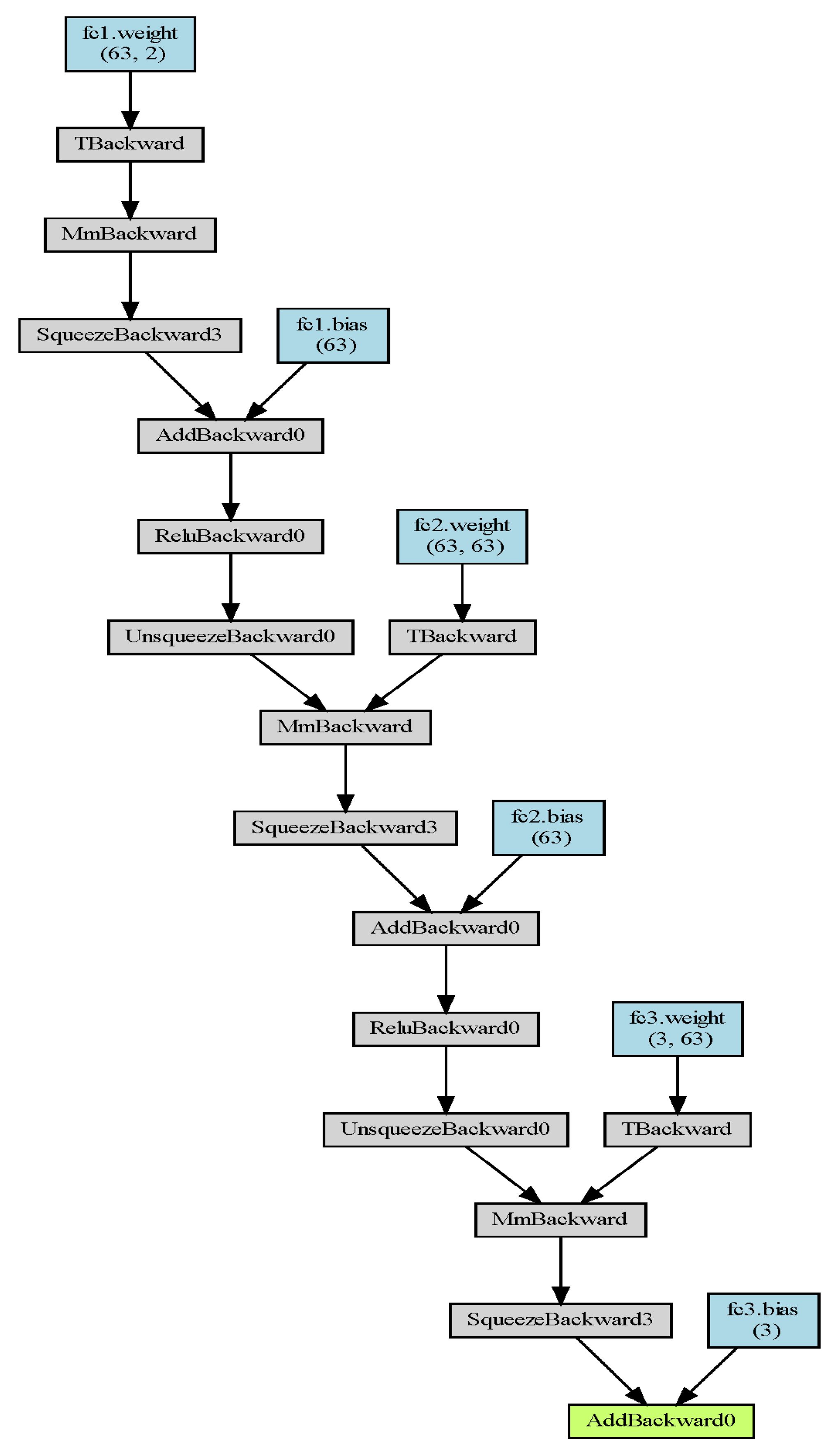
The specific network structure can be seen in
Figure 3, where the linear layer has three layers and the nonlinear layer has two layers, and the Relu function is adopted.
Where we use Pytorch to build the network model, the Adam optimizer is used. The specific hyperparameters settings can be seen in
Table 1.
4.1. Learning Rate Order of Magnitude Initial Determination
In the experiment in this paper, a Deep Q-Network (DQN) algorithm is implemented by using a neural network and compared from this baseline. In fact, we can generalize to other TD algorithms by using this as a baseline.
From our analysis of the mathematical model in the first two sections, we can see that when
, there is
. However, in practice, such a setting is unreasonable. First, when
, the learning rate goes to 0. Such a setting cannot make the neural network update and converge. Secondly, the convergence of the neural network also depends on the learning rate to a great extent in the actual use. Taking the ideal convex optimization as an example [
27], the convergence process of the reasonable gradient optimization should continuously descend along the direction of the gradient. However, when the learning rate is too small, it will theoretically lead to too slow convergence of neural network parameters, which will affect the convergence rate of the neural network. At the same time, too much setting of the learning rate leads to deviation of gradient descent direction and even makes it difficult to converge eventually. Therefore, in the deep reinforcement learning, we should set a uniform learning rate test interval, to select a more appropriate learning rate parameter in the case of fewer test training times.
The method used in this article is called cross-magnitude initializations. That is, we set a test parameter at each order of magnitude after the decimal point. In order to ensure the premise that the learning rate tends to 0, we locate the test learning rate of each order of magnitude test interval at 1. For example: 0.1, 0.01, 0.001…The optimal learning rate is selected through the test, and the optimal interval is selected through the final accumulative income and convergence effect. In the experiment, we set a time of 1000 turns for interacting with the environment, and a maximum of 200 steps are performed in each turn. We record the average return per 100 episodes. Take the highest average return as a measure of agent rationality [
29]. We have counted the results of ten experiments with different learning rates, and the results are shown in
Table 2.
From our experiments, it can be seen that the order of magnitude of the appropriate learning rate should be between three decimal places and the last four places. We call this the “appropriate learning interval”. Accordingly, we selected the selected range of the appropriate learning rate preliminarily.
4.2. Convergence and Rationality Are Combined to Determine the Learning Rate
In this section, we further select the appropriate learning rate interval. Different from the traditional simple setting, we not only consider the accumulated income of the algorithm as the negative feedback to form a closed loop. We also consider adding convergence as another condition for the negative feedback loop.
In machine learning and deep neural network training, the error value is usually used to determine whether the algorithm converges or not [
34,
35]. Although unlike traditional supervised learning, reinforcement learning does not have a deterministic target value (supervised learning), the purpose of the algorithm is to approximate the optimal value function. Therefore, in the TD algorithm, the TD error can be similar to the error used in the network parameter update in supervised learning. Therefore, it can be used as a measure of convergence performance of the algorithm [
23].
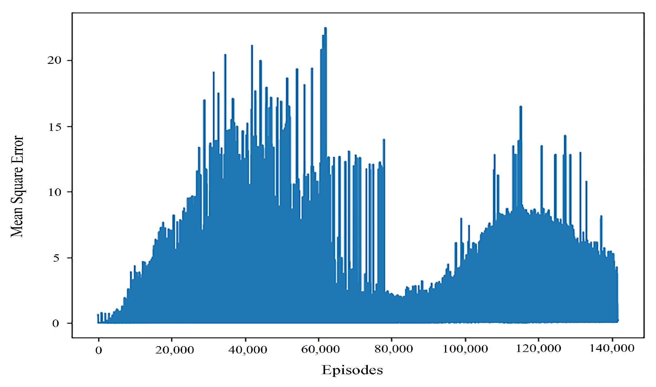
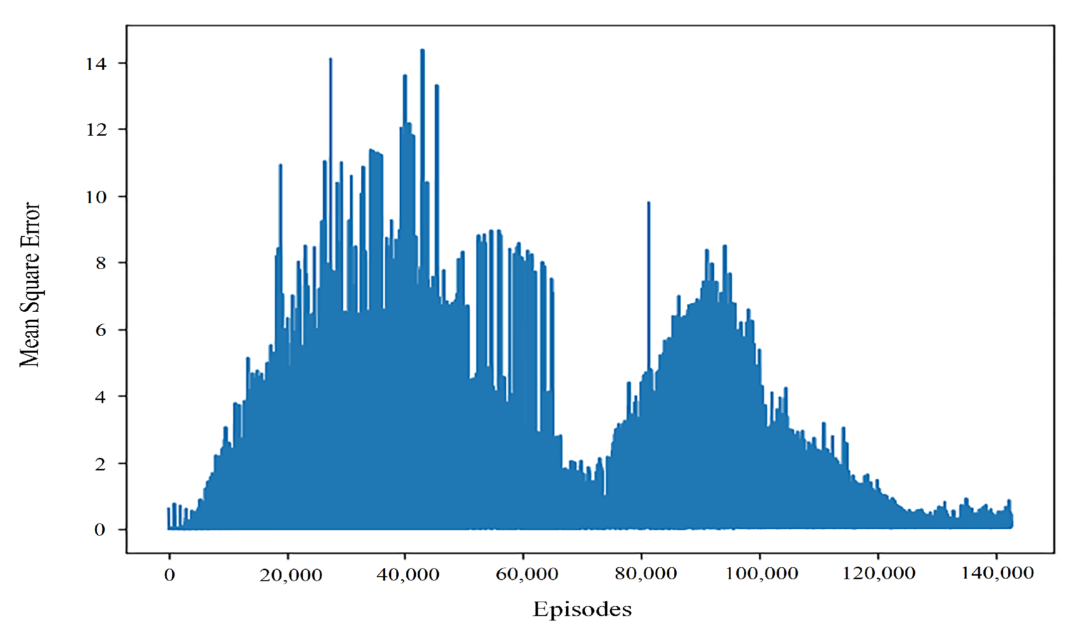
By comparing the typical values of controller returns and convergence results of learning rate training of different orders, it can be seen that even when the return values are close, the convergence performance of the algorithm is still quite different. As can be seen from
Figure 4, when the learning rate is 0.001, the algorithm can quickly obtain better results, but in the later stage of interaction with the environment, the performance stability of the algorithm is poor. This may be because the learning rate is more sensitive to the gradient in the later stage of the algorithm. The mean square error when the learning rate is 0.0001 and the convergence effect is good can be seen in
Figure 5.
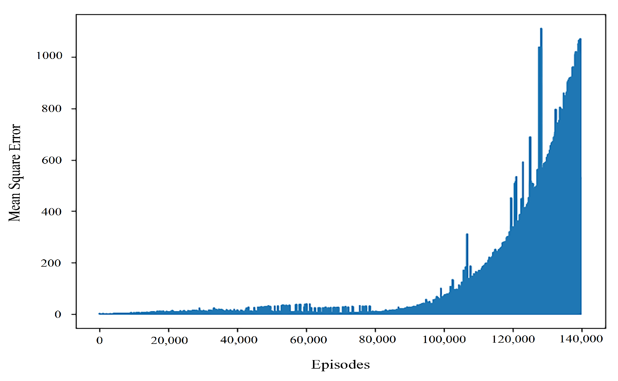
At the same time, when the learning rate is 0.0001, the convergence speed of the algorithm is slow. However, it can be seen that once the algorithm converges, the error was better in a large number of experiments. However, in most cases in our experiment, when the learning rate is 0.0001, the typical variation value of the mean square error is shown in
Figure 6.
It can be seen that when the learning rate is at the magnitude of 0.0001, although the algorithm can have a better return value, it is difficult for the algorithm to converge in the later stage of training. It makes it hard to stabilize the result. At the same time, we also conducted a test in this order of the learning rate. Comparatively speaking, the learning rate at 0.0002 can appear to have more stable convergence training results. Therefore, when we dynamically adjust the learning rate, we add 0.0002 to maintain the stability of the learning rate at this order.
Our ultimate goal is that the algorithm can approach the optimal result quickly in the early stage and maintain stable convergence results in the later stage. A large number of experimental results show that this performance is difficult to obtain by the static learning rate. Therefore, we want to break through the effect of the original static learning rate algorithm by dynamically adjusting the learning rate of the algorithm and combining the different advantages of various learning rates at different stages.
During the interaction between agents and the environment, to increase the exploration of actions in the early stage and stability in the later stage, we adopted the method of epsilon-greedy in the selection of action strategies. At the same time, dynamically adjusting the learning rate makes the error as close to the theoretical value as possible and presents a trend of gradual decline. Finally, a more stable training model (controller) is obtained to adapt to the final controlled system. It can be seen from the variation trend of the training mean square error, when comparing the learning rate of 0.001 and 0.0001, that in the early stage of training, a large learning rate can enable the algorithm to converge quickly to the target result. However, in the later stage, the difference error of timing sequence is small, and too much learning rate will lead to the instability of the algorithm. Therefore, in the later stage of training, a small learning rate can ensure the convergence of the algorithm. Paper [
23] combined with the idea of the Hysteretic Q-Learning (HQL) algorithm, the learning rate of the algorithm is fixed when the TD error is positive. When the TD error is negative, the method is dynamically adjusted. In theory, we can get a better result called the former static learning rate method. After analyzing the timing error distribution, we set the algorithm’s dynamic learning rate as shown in
Table 3.
4.3. Experimental Results and Analysis
In this part, we show the difference in rationality and convergence between static learning rate and dynamic learning rate algorithms.
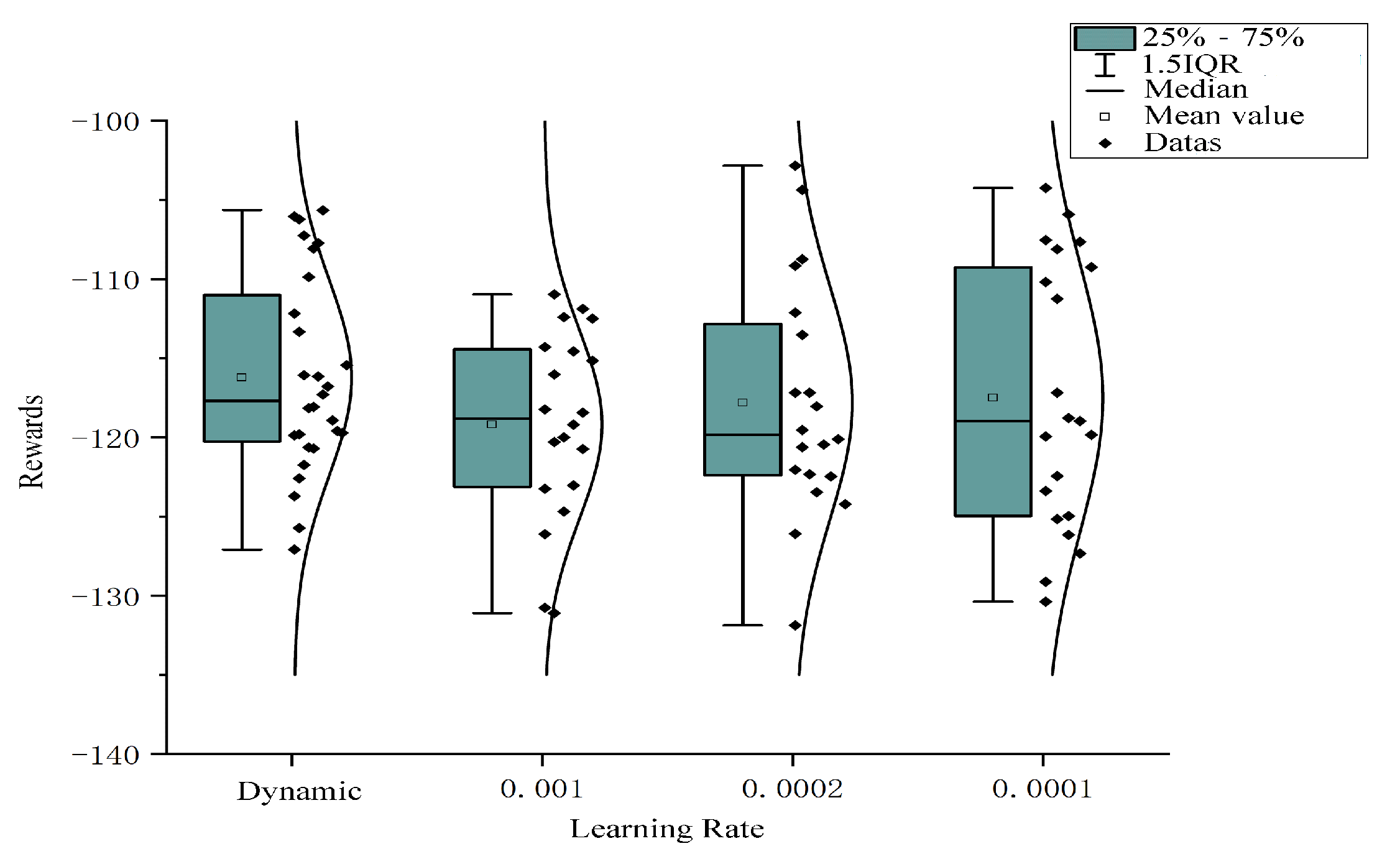
In order to avoid interaction with the environment, agents appear as extreme phenomena. We have conducted a large number of experiments on the results of static learning rates 0.001, 0.0001, 0.0002, respectively. The results can be seen in
Figure 7.
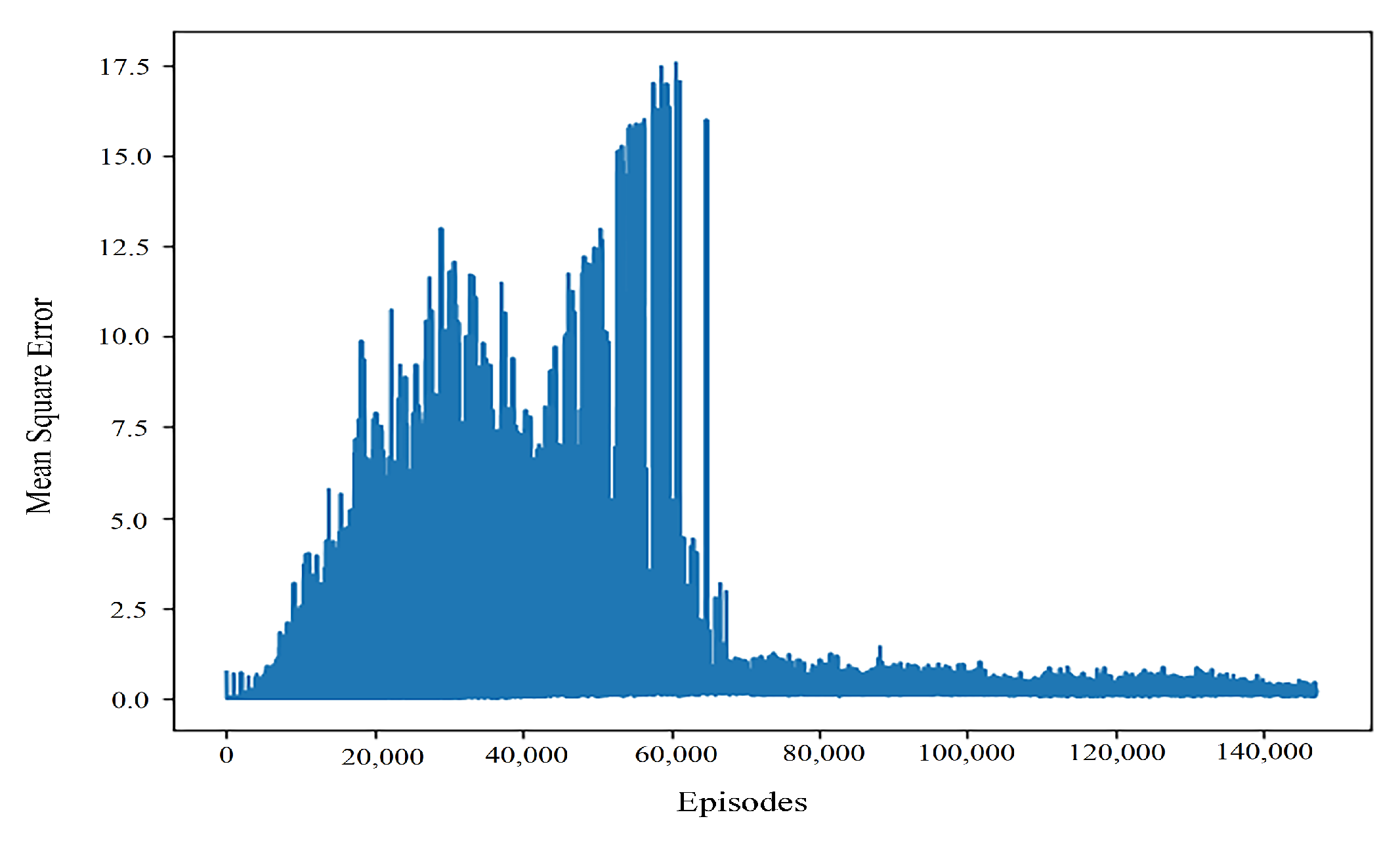
To show the results without loss of generality, the distribution of the results with different learning rates and 75 percent confidence intervals and mean values of the algorithm are shown in the figure. It can be seen that the learning rate algorithm of dynamic regulation is the optimal one. In terms of the overall stability of the algorithm training, the performance difference of the dynamically adjusted learning rate algorithm is small. Although the optimal result is in the static learning rate of 0.0001, its distribution is discrete and can be considered as noise points and ignored. Therefore, it can be considered that the optimization of the dynamic regulation algorithm to the traditional static learning rate algorithm is significant. At the same time, we can compare the stability of the algorithm in the network update by means of the mean square error. The general variation of the mean square error of the improved algorithm can be seen in
Figure 8.
To sum up, it can be seen that the algorithm that dynamically adjusts the learning rate can combine the advantages in different stages in the training process. Under the condition of ensuring the performance of the basic learning algorithm, the profitability and convergence results of the algorithm can be improved. The convergence results can be obtained from the stability of the final results obtained by the algorithm and the neural network error. This also proves that the method of dynamically adjusting the learning rate can improve the effect of the algorithm to a certain extent.
5. Conclusions
This paper proves the feasibility of dynamic adjustment learning rate in a reinforcement learning algorithm. At the same time, it solves the problem of setting learning rate parameters of reinforcement learning to a certain extent. By combining the advantages of different learning rates in different intervals, the algorithm can break through the original optimal effect. We prove that the learning rate of dynamic adjustment can ensure the convergence of the algorithm in theory. In the experiment, we have verified the effect of this method on adjusting the learning rate. The results show that the method of dynamically adjusting the learning rate can break through the original static learning rate algorithm and achieve a stable income effect. This algorithm has a considerable improvement in both the convergence performance of the network and the return results of the algorithm convergence in practice.
To date, it is still difficult to find a suitable rule for the deep neural network and the parameter adjustment method using a neural network. The method of dynamically adjusting the learning rate proposed by us is an algorithm that can adapt to the reinforcement learning model. It combines the unique characteristics of reinforcement learning and a dynamic programming model and adopts a static hyperparameter setting method different from the traditional neural network (supervised [
36] and unsupervised learning [
37]). Comparing with the static learning rate, the method of dynamic adjustment of learning rate can combine the advantages of different learning rates. In this paper, the dynamic regulation is based on the dynamic matching of the TD error, and the effect of the algorithm is verified in the experiment. It can be seen from a large number of experimental results that the algorithm without loss of generality, which dynamically adjusts the learning rate, is superior to the reinforcement learning algorithm with traditional static learning rate in terms of the performance of mean value and distribution. At the same time, it can also be seen from the mean square error loss that the dynamic adjustment algorithm optimizes the cumulative rewards and stability of the original algorithm. The results show that the algorithm of dynamically adjusting learning rate is a kind of hyperparameters setting rule that is more suitable for deep reinforcement learning. The defect of this paper is that there is no quantitative explanation of the relationship between specific learning rate and agent rationality and convergence. To some extent, the method we studied can solve the problem of a large network error scale in the later stage, but it cannot completely avoid the fluctuation of a network error. In other words, this method can achieve “stable” results within a certain error tolerance range and shows that the basis for dynamically adjusting the learning rate is not only a temporal-difference error. This is instructive to the traditional reinforcement learning parameter regulation, and it also means that our method is worthy of further study. In future work, we will further study the coupling relationship between the convergence of deep reinforcement learning and the algorithm’s cumulative return. Given the defect that this paper does not propose the relationship between quantitative analysis of cumulative return and update error, we will do further research.


