Article

Study on Multi-Objective Optimization-Based Climate Responsive Design of Residential Building

School of Architecture, Tianjin University, Tianjin 300072, China
*
Author to whom correspondence should be addressed.
Algorithms 2020, 13(9), 238; https://doi.org/10.3390/a13090238
Submission received: 24 August 2020 / Accepted: 17 September 2020 / Published: 21 September 2020
(This article belongs to the Special Issue Metaheuristic Algorithms in Engineering Optimization Problems)

Abstract

:
This paper proposes an optimization process based on a parametric platform for building climate responsive design. Taking residential buildings in six typical American cities as examples, it proposes thermal environment comfort (Discomfort Hour, DH), building energy demand (BED) and building global cost (GC) as the objective functions for optimization. The design variables concern building orientation, envelope components, and window types, etc. The optimal solution is provided from two different perspectives of the public sector (energy saving optimal) and private households (cost-optimal) respectively. By comparing the optimization results with the performance indicators of the reference buildings in various cities, the outcome can give the precious indications to rebuild the U.S. residential buildings with a view to energy-efficiency and cost optimality depending on the location.

1. Introduction

In recent years, the parametric simulation of building performance has gradually become a common method in the field of building energy-saving design. Social and economic development requires sustainable building design to achieve low energy consumption on the premise of ensuring a high-performance building environment. Thus, building energy-saving design cannot sacrifice performance for low energy consumption. Increasing attention has been paid to the impact of the indoor environmental performance of residential buildings on the physical and mental health of residents. As the pursuit of improving the performance of a single environment often adversely affects the performance of other aspects, the research on multi-factors environment and its coupling performance has grown fast. Multi-variable energy-saving design scheme and process is more complicated than the single-variable energy-saving strategy, the value and significance of the multi-variable design have also greater effect on building performance improvement. In addition, from the perspective of architectural design, the design strategy proposed based on a single objective (such as improving indoor lighting environment, ventilation, solar shading, etc.,) during the schematic design stage does not fully conform to the architect’s way of thinking and cannot effectively facilitate the building design. Therefore, it is necessary to establish the relationship between multi-variable design elements and multi-objectives, in order to setting up an integrated and systematic analysis framework.

2. Background and Literature

2.1. The Logic of Building Climate Responsive Optimization Design

The building climate responsive design strategy aims to study the climate control methods applicable to the building comfort space. By considering the climate differences in different places and using appropriate strategies to improve the occupants’ thermal comfort, the building environment is adjusted in order to providing a comfortable indoor thermal environment for human daily activities. In this method, the choice of building technology is based on the relationship between external climatic conditions and human needs [1,2,3].
In order to quantitatively analyze the environmental benefits of building climate responsive design, the research proposes an optimization process based on building simulation, integrates building performance simulation and optimization, and implements a reverse search for optimal performance parameters. Architectural design is essentially an optimization problem. Architects are constantly improving the design based on existing means to meet the design requirements in the best way which is an iterative process [4,5]. In general, the design process can be divided into two main stages: the divergent stage, which is mainly to generate conceptual alternatives; and the convergence stage, which is mainly used to evaluate and select the best conceptual design from the proposed alternatives. In all stages of design, from the conceptual design stage to the detailed design stage, the steps of divergence and convergence are always repeated. Until the end of the design phase, the number of alternatives gradually decreased, leaving only one or a few solutions. This iterative process is the process of design exploration, which aims to study and develop the design space and provide information for decision-making throughout the design process, as shown in Figure 1.
The traditional architectural design process does not have an integrated system and method in the early scheme divergence stage and the late convergence stage. Architectural design in the traditional sense is always judged based on the architect’s experience, and the architect’s cognitive level determines whether the project can achieve the expected objectives. When the design problem involves a large number of complex variables, it is difficult to achieve the optimal goal only by the architect’s subjective judgment. The development of today’s building simulation technology can effectively assist designers in making decisions to eliminate uncertain assumptions in the design process to a certain extent, and quantitatively evaluate the design scheme. However, these procedures are quite complicated, and the data required for calculation is very detailed, which is difficult to obtain in the early stage of the design, so the relevant scheme can only be evaluated in the later stage of the design. Most of the decisions that have a significant impact on energy consumption are made in the early design stage. Therefore, in the traditional design process, it is difficult to effectively assist the building climate responsive design by relying solely on these simulation programs [6,7].
The study proposes the use of optimized search methods based on building environment simulation. More in detail, based on building simulation tools, a Monte Carlo simulation framework was established to analyze and search the uncertainty of the input parameters, and use automation to solve the problem that it is difficult to determine the input parameters in the traditional sense. Optimization is the process of finding the best combination of different solutions when the given constraints are met. The execution of optimization requires decision variables, objective functions, and constraints. The Equation (1) expresses the general mathematical optimization process.
minx ∈ Rnƒ(X)
Subject to: gi(X) ≤ 0, i = 1, 2, …, m
Kj(X) = 0, j = 1, 2, …, p
where, X represents different decision variables, ƒ(X) are objective functions, constraints are gi(X) ≤ 0, I = 1, 2, …, m and Kj(X) = 0, j = 1, 2, …, p. Determining decision variables, objective functions, and constraints are the most important parts of the optimization process, and different optimization algorithms can be selected based on the classification of different objective functions and constraints.
The optimization method can effectively search for solutions, so as to realize the automation and integration of design simulation. The traditional “forward” design process follows the energy evaluation process in the building design process. The user selects the values of decision variables (such as building size, materials, and climate data), inputs the data into the physical model, then calculates and outputs energy performance predictions. In the forward process, a set of known design parameters is required, from which the user can estimate performance. However, in the early stages of design, the design objectives have been determined, and the user aims to seek designs that meet the performance goals. Therefore, the “inverse” modeling process that uses the goals to infer the design parameter values is more in line with the nature of the earlier design stage.
In the reverse workflow of early design, performance preferences and boundary conditions (such as weather and building type) are known, and the values of decision variables are unknown. The following Equation (2) expresses the method of inverse modeling search. Assuming that y is a performance index, the thermal load model of the building can be expressed as:
y = ƒ(x1, x2, x3, …, xn) = ƒ(xdesign, xscenario)
where y is a function of different decision variables xi, like building orientation and shape coefficient which can be divided into two groups, i.e., design parameter variables and scenario variables. Design parameter variable xdesign represents the parameter variable of architectural design, while the scenario variable xscenario contains boundary conditions related to building operation and climate parameters. ƒ is corresponding to energy simulation tools which calculates the value of a given decision variable x based on a physical function. By function ƒ, forward modeling can find y through given x (as in Equation (3)), while reverse modeling finds multiple x through given y (as in Equation (4)).
x: (x1, x2, x3, …, xn) design parameters→y:performance (forward modeling)
y: performance→x: (x1, x2, x3, …, xn) design parameters (reverse modeling)
In the initial stage of design, there are many design and scene parameters x that have not yet been determined. In this case, the probability distribution relationship between x and y within the possible range can be obtained using a probabilistic method. Figure 2 graphically represents the logic of the current deterministic forward model (Figure 2a), the probabilistic forward model (Figure 2b), and the probabilistic reverse model proposed in this study (Figure 2c).

2.2. State-of-the-Art

There are many scholars in the field of building optimization by integrating rhino, grasshopper (GH), building performance simulation plug-ins (such as DIVA) and GH evolution solver: Galapagos, to conduct building performance optimization, including building energy-efficient skin optimization, high performance building system optimization, building orientation optimization, building operations optimization, life cycle assessment and alternative energy applications [8,9,10,11], etc. However, in the GH platform, Galapagos can only optimize one objective function at a time, so when dealing with architectural multi-objective optimization problems, it is necessary to reprocess the data results, or use other evolutionary solvers of the platform, such as Octopus.
For the multi-objective building optimization, Asadi et al. [12] proposed another operation process, that is, using TRNSYS, GenOpt, and Tchebycheff optimization technology developed in MATLAB to simulate and optimize the building environment.
Asl et al. [13] also explored Revit’s plug-in Dynamo to extend the parametric functions of the platform. They also used NSGA-II’s free software package Optimo to solve optimization problems.
In terms of research on building renovation and design by multi-objective optimization methods, Giovanni Pernigotto et al. [14] defined the decision variables and their ranges based on the lowest building energy consumption and the lowest investment cost to achieve the best combination of renovation parameters. The strategies mentioned in this study are common measures for building renovation, such as the thermal insulation performance of external walls and windows, the size of windows and the lighting effect of glass, etc., which are convenient for large-scale popularization and application.
Tomás Méndez Echenagucia et al. [15] investigated the open space of office buildings, including location, shape, window type and thickness of masonry walls as decision variables, using EnergyPlus and NSGA-II algorithm (Non-dominated Sorting Genetic Algorithm) for building environment simulation and multi-objective optimization to search Pareto frontier for building energy efficiency design.
Alessandro Prada and Giovanni Pernigotto et al. [16,17] discussed the robustness of the optimal solution obtained by GA multi-objective optimization to the quality of the weather data used. Using the climate parameters of six different reference years in Trento and Monza in northern Italy, they applied four energy-saving measures related to building envelopes and HVAC systems to six typical building types, and studied when to adopt NSGA -II Genetic algorithm selects the most cost-effective building energy-saving renovation measures, to what extent the uncertainty of typical weather conditions will affect the results of building energy-saving renovation and TRNSYS simulation.
Paola Penna et al. [18] evaluated the optimal combination of building energy efficiency measures (EEM) by using multi-objective optimization algorithms and dynamic simulation tools to achieve the results of economic optimization, minimum energy consumption and maximum thermal environment comfort.
Based on the perspective of architectural design, the research on the climatic responsive design of residential buildings presents a trend of gradually deepening and refining over time, which is reflected in the following characteristics:
(1)
From energy-saving design practice or theoretical research based on qualitative analysis to energy consumption simulation based on quantitative research.
(2)
Research related to building energy consumption is becoming more and more comprehensive, from only focusing on building thermal performance or energy consumption of air conditioning systems to a comprehensive evaluation system that also considers other factors such as total building energy consumption, lighting, and indoor thermal comfort, etc.
(3)
The research of building energy-saving design variables usually manifests as the research of single variable and multi-variable combination. The research of single variable is an indispensable basic part, and the combination of multi-variable constitutes the final goal of the research and a complete building energy-saving design process.
(4)
“Performance coupling factor” has been paid attention to, and the impact of indoor building environmental performance quality on the physical, mental health and comfort of residents has been paid more and more attention. The pursuit of a single environmental performance improvement often has an adverse effect on other aspects of performance, related researches on multi-factors environment and its coupling performance are getting increasing attention.
(5)
New tools or methods for building energy consumption simulation combined with parametric methods, BIM technology or computer programming technology are constantly emerging. On this basis, the amount of simulated data is increasing, and the reliability of the simulation results is improving.
Multi-variable energy-saving design schemes and processes are more complicated than single-variable energy-saving strategies, and under the combined effect of multi-variables, the value and significance of building performance improvement are also greater. In addition, based on the perspective of architectural design, the design strategy proposed based on a single objectives (such as improving indoor lighting environment, ventilation or solar shading) during the schematic design stage does not fully conform to the architect’s way of thinking and cannot effectively facilitate the building design. Therefore, it is necessary to establish the relationship between multi-variable design elements and multi-objectives, in order to building an integrated and systematic analysis framework.
For building climate responsive design, energy consumption, indoor thermal environment and building life cycle cost are three conflicting basic factors. Generally speaking, to make the indoor thermal environment satisfy the human comfort as much as possible, it will lead to an increase in building energy consumption and costs. The three often contradict each other, while in the decision-making process, it is crucial to trade off these three objectives. If the building energy consumption and life cycle costs are required to be reduced while maintaining the indoor thermal environment, it is necessary to carry out quantitative prediction and multi-objective optimization of the built environment factors.
Based on the meteorological parameters and design codes of typical cities in different climatic regions in the United States, a framework for optimizing the climate responsive design parameters of residential buildings in typical cities has been established. Building energy demand, thermal comfort, and life cycle costs are used as performance indicators to analyze optimal energy-saving design of residential buildings in U.S. typical cities.

2.3. Research Objects and Optimization Process

The United States is located in the Western Hemisphere which is composed of the United States, Alaska, and Hawaii. East and West are adjacent to the Atlantic and Pacific ocean. Because of the vast territory of the United States, it is one of the countries with the most climatic types in the world. Most of the climate of the United States is temperate and subtropical, and only the southern end of the Florida Peninsula is tropical. Alaska is located between 60 and 70 degrees north latitude and is a cold climate zone within the Arctic Circle. Hawaii is located south of the Tropic of Cancer and is a tropical climate zone. The United States divides the country into eight different main climate types as shown in Figure 3 [19].
Because of the diverse and complex climate types in the United States, the study only selected typical cities in the United States’ six climatic regions for analysis. Figure 4 shows the geographic location of typical cities on the map of the United States. Table 1 lists the heating period of typical cities based on the actual heating survey in each city.
The building climate responsive analysis in this study is based on an integrated parametric simulation process. The research proposes a multi-objective optimization process based on parametric simulation of building performance, which consists of two parts and is divided into three steps, as shown in Figure 5. The data collection and generation steps constitute Part 1: Design prototype generation. The optimization steps constitute Part 2: design optimization. Part 1 collects specific design parameters, such as building shape coefficients, window-to-wall ratios, etc., as well as the default parameters, such as constraint parameters, etc., used to generate design prototypes. Part 2 optimizes the architectural design prototype generated in Part 1. The result of this process is a series of optimized architectural design solutions for designers to evaluate, select and further develop. For building climate responsive design, the result is a building design solution with high thermal comfort and low energy consumption, which can be embodied in the process shown in Figure 6.
This research is based on the Rhino/Grasshopper parametric platform, using Ladybug and honeybee environment analysis plug-ins to conduct modeling analysis of the building environment and energy demand. The application of this workflow can be shown in Figure 7 below.

2.4. Algorithm Used in Optimization

Currently in multi-objective optimization research, representative algorithms include MOGA (Multi-Objective Genetic Algorithm), NSGA (Non dominated Sorting Genetic Algorithm), NSGA-II (Non dominated Sorting Genetic Algorithm-II), PESA (Pareto Envelope-Based Selection Algorithm), and SPEA-II (Strength Pareto Evolutionary Algorithm-II). The performance of multi-objective algorithms mainly depends on three aspects, namely convergence, the distribution of solutions set and robustness. NSGA-II, SPEA-II, and PESA all have good convergence and stability, but compared with SPEA-II and PESA, NSGA-II has worse convergence. Because of the truncation characteristics in NSGA-II algorithm, its distribution performance is obviously not as good as SPEA-II. Furthermore, when the number of targets is more than one, PESA will have poor distribution. It can be seen that the SPEA-II algorithm is superior to other algorithms in terms of convergence and solution set distribution. Therefore, the SEPA-II algorithm is used in this study.
SEPA2 is an improved version of SPEA (Strength Pareto Evolutionary Algorithm) proposed by Zitzler and Thiele in 2001 [22]. It is a Pareto algorithm for solving multi-objective problems. In this algorithm, the fitness of an individual is also called Pareto strength. The fitness of individuals in a non-dominated set is defined as the proportion of the total number of individuals dominating in the group. The fitness of other individuals is defined as the total number of individuals dominating it plus one, and individuals with low fitness are corresponding to a higher probability of selection. In addition to the evolutionary population, an external population is also set up to save the current non-dominated individuals. When the number of individuals in the external population exceeds the predefined value, clustering techniques are used to delete them. Tournament is used to select individuals from evolutionary groups and external populations to enter the mating pool for crossover and mutation operations.
The SPEA-II algorithm flow chart is shown in Figure 8 and Figure 9. Suppose the size of the group P is N, the archive set Q is M, and the number of iterations is T, then the work flow of the SPEA-II algorithm [23] is:
(1)
Randomly generate an archive set and initial population Q0, P0, and iterator t = 0.
(2)
Calculate fitness for individuals in PT and QT.
(3)
Keep all non-dominated individuals in PT and QT into the next generation archive set QT+1. If |QT+1| > M, then remove excess individuals. If |QT+1| < M, then select some individuals in PT and QT, to join QT+1 to make |QT+1| = M.
(4)
If t = T or other termination conditions are met, the non-dominated solution in QT+1 is output as the algorithm result.
(5)
If not satisfied, perform tournament selection, crossover and mutation on QT+1, keep the result in PT+1, t = t + 1, and back to (2).
The logic of fitness allocation and environment selection is as follows:
(1) Fitness allocation
In order to make each individual have a different fitness value, while considering the situation of all individuals in the iterative group and the external group. The crowding situation is determined by calculating the distance between an individual and its neighbors, that is, calculating the fitness of each individual in the population PT (initial set) and QT (archive set). The total fitness F(i) is determined by R(i) and D(i) (as in Equation (5)).
F(i) = R(i) + D(i)
where R(i) is the integer part, and R(i) is calculated as Equation (6).
R ( i ) = j P t Q t , j i   S ( j )
where S(j) is the number of individuals dominated by j in the population Pt and QT. The lower the R(i), the better the quality of the solution. D(i) is the decimal part, and its calculation is as shown in Equation (7).
D ( i ) = 1 σ i k + 2
where σik is the distance from individual i to its k-th nearest individual, and 2 is added to the denominator is so that the distance is not 0 and D(i) < 1. K = √|Pt| + |Qt|, which select the non-dominated solution set of the current iteration population and the external population. When the number of the external population is greater than the preset value, delete the poorer individuals in the external population. Otherwise, the better individuals in the iteration population are selected to supplement. Repeat this process until the size of the external population reaches the preset value.
(2) Environment selection
Select suitable individuals from the population Pt and QT and store them in the next-generation archive set QT+1. If |QT+1| ≤ M, choose the smallest remaining F(i) from Pt and QT to join them until |QT+1| = M. If |QT+1| > M, then use archive pruning to continuously delete individuals in QT+1 until |QT+1| = M. Meanwhile, σik is used to evaluate distance among different individuals, and delete the individual with the smallest distance from the selected one, as shown in Figure 10.

3. Multi-Objective Optimization Platform Set-Up

3.1. Definition of Objective Functions

Building climate responsive design aims to ensure the comfort of the building’s thermal environment while reducing building energy consumption and life cycle costs as much as possible. Therefore, the thermal environment comfort model, building energy demand model and building life cycle cost model are the three important aspects of climate responsive design. To some extent, these objective functions are both interrelated and conflicting. The basic parameter settings of these three objective functions for building climate responsive design are defined as follows:
(1) Thermal environment comfort
The international standard ASHRAE 55 [24] defines “thermal comfort” as: a state of consciousness in which a person expresses satisfaction with the thermal environment, which is affected by differences in personal emotions, individual physiological structures, climate, culture, and society, etc. Thermal comfort is a relative concept. There is no absolute thermal comfort. Comfort is a subjective psychological state. It cannot be determined because it cannot be measured objectively and changes constantly according to various factors. Based on a series of parameter settings, the study uses the PMV model to calculate the annual Discomfort Hours percentage (DH) as an indicator for thermal environment comfort assessment.
According to the typical activity levels and clothing thermal resistance values listed in ANSI/ASHRAE STANDARD 55-2013, the research roughly determined the input parameters of clothing thermal resistance values for simulation. The step value changes according to the change of the monthly external average temperature. The metabolic rate is fixed at 1.2 met in the case, which corresponds to the sedentary behavior in residential buildings. In addition, the air speed is set to a very low speed of 0.05 m/s, which is more common in most enclosed indoor environments. The specific input parameters for PMV calculation vary with monthly steps, as shown in Table 2. Table 2 lists only a few fixed values that do not need to be changed in EnergyPlus calculations, namely indoor air speed, clothing thermal resistance, and human metabolic rate. The indoor air temperature, relative humidity and average radiant temperature vary with parametric simulation which needs to be read after calculation by EnergyPlus and cannot be set in advance.
(2) Building energy demand
The climate responsive design optimization in this paper only focuses on passive design strategies. Passive design strategies can be controlled by the architect during the design phase, or adjusted by the user during the operational phase. Other mechanical system parameter setting are beyond the scope of this research. Therefore, the annual building energy demand is defined as the sum of the cooling and heating loads of all apartments, [25,26,27,28] domestic hot water, electrical equipment and other energy needs are not included in the calculation. The cooling period in summer and the heating period in winter are set according to the requirements of different climate zones. In this study, in order to avoid the influence of HVAC system parameters, its performance coefficient is assumed to be 1, so the energy demand can be directly extracted from the EnergyPlus simulation results. It is assumed that no heat recovery device is implemented in the HVAC system. Therefore, the objective function of the annual building energy demand can be calculated as Equation (8):
BED = 1 A i = 1 n ( E c i + E h i )
where BED represents the annual building energy demand per unit building area (kWh/m2), the calculation of building energy demand only considers heating and cooling demand, and does not consider other aspects, such as lighting, domestic hot water, etc. Eci is the cooling demand of the i-th floor, Ehi is the heating demand of the i-th floor, n is the total number of floors in the building, and A is the total area of each floor in the air-conditioning area of the building.
(3) Building life cycle cost
In order to assess the total cost associated with a given building, a life cycle cost analysis (LCCA) was performed using a 30-year time scale [29,30]. The full life cycle cost of a building includes initial construction costs, annual energy use costs, and ongoing maintenance costs. However, according to the concept of global cost, in the current research for the schematic design stage, only building materials and annual energy costs are considered because they have the greatest impact on life cycle costs. Equations (9)–(11) shows the method used to calculate the life cycle cost in this study.
G C = C I + i = 1 30 [ C e , i R d ( i ) ] A
Rd(i) = [1 − (1 + Rr) − i]/Rr
Rr = (Ri − Re)/(1 + Re)
where GC represents building life cycle global cost, in $. CI represents initial investment cost, in $. Ce,i is the energy cost of the ith year, in $. Rd(i) is the discount rate of the ith year. A is the total area of each floor, in m2. Rr is the effective interest rate, Re is the rate of increase in energy prices, which is assumed as 1.2%. Ri is the market interest rate, which is 4.25% [31]. The calculation period is 30 years because the accuracy of economic calculation results beyond 30 years will be affected. During the calculation period, it is assumed that the energy demand of the building remains unchanged.

3.2. Design Parameter Settings of Typical Buildings

The typical model established by the research is an ordinary two-story residential building (see Figure 11). The specific parameters are shown in Table 3. The design parameters of the building envelope are shown in Table 4.
Based on the typical model, the optimization mainly focuses on the design parameters of the building envelope. The HVAC system, primary energy, and renewable energy system under the optimization framework are fixed (i.e., not included in the optimization process). The design parameters of the envelope are shown in Table 5 and Table 6, and the initial investment cost calculation is shown in Table 7.
With the help of integrated parametric software, various parameters used for building energy modeling can be collected and analyzed on the same platform. The research uses the plug-in Octopus of Grasshopper to search the target function value. Octopus applies the evolutionary principle of SPEA-2 to the process of parametric design, and produces a series of trade-off solutions between the extreme values of multiple targets. The operation flow of Grasshopper is shown in Figure 12.

3.3. Design Parameter Settings of Typical Cities in the United States

According to the U.S. climate zone, six different typical cities are selected, as shown in Table 8. Refer to the international energy conservation regulations IECC formulated by the International Code Committee [21], Table 9 lists the design parameters of the reference buildings envelope in each typical city according to the design code in the climate zone where the typical city is located, for comparison with the optimal design parameters of each city. According to the settings in Table 9, Table 10 calculated the design parameters of the reference buildings in each city by typical model, and obtained the performance indicators shown in Table 11.

4. Discussion of Optimization Results

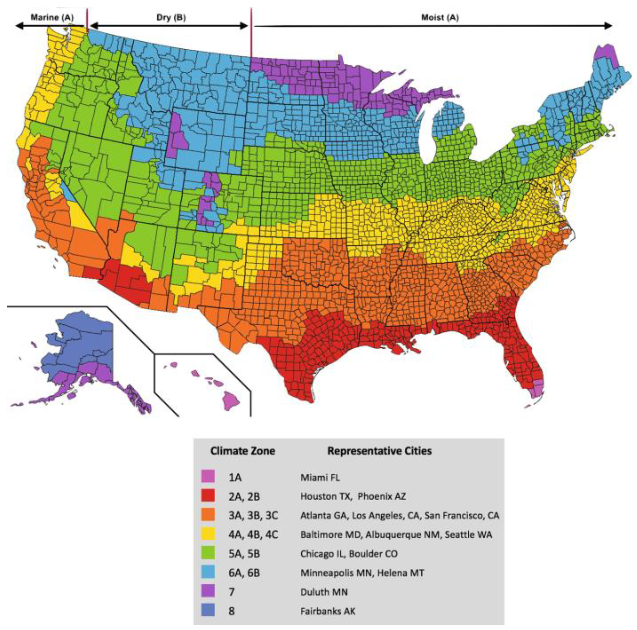
Based on the above multi-objective optimization logic, this section conducts climate responsive optimization analysis for typical cities in six different climate regions in the United States. As above mentioned, the objective functions are discomfort hours percentage (DH) for thermal environment evaluation, building energy demand (BED), and building life cycle global cost (GC). The optimized parameter results and performance indicators of residential buildings in various U.S climate zones are compared and discussed.

4.1. Optimization Results of Residential Buildings in Typical American Cities

Figure 13 shows the optimization process with Duluth as an example. From the figure, it can be seen that the Pareto frontier of multi-objective optimization is more and more dense before the 9th generation, and then gradually begins to converge until the 30th generation. After 30 generations, the Pareto front has hardly changed.
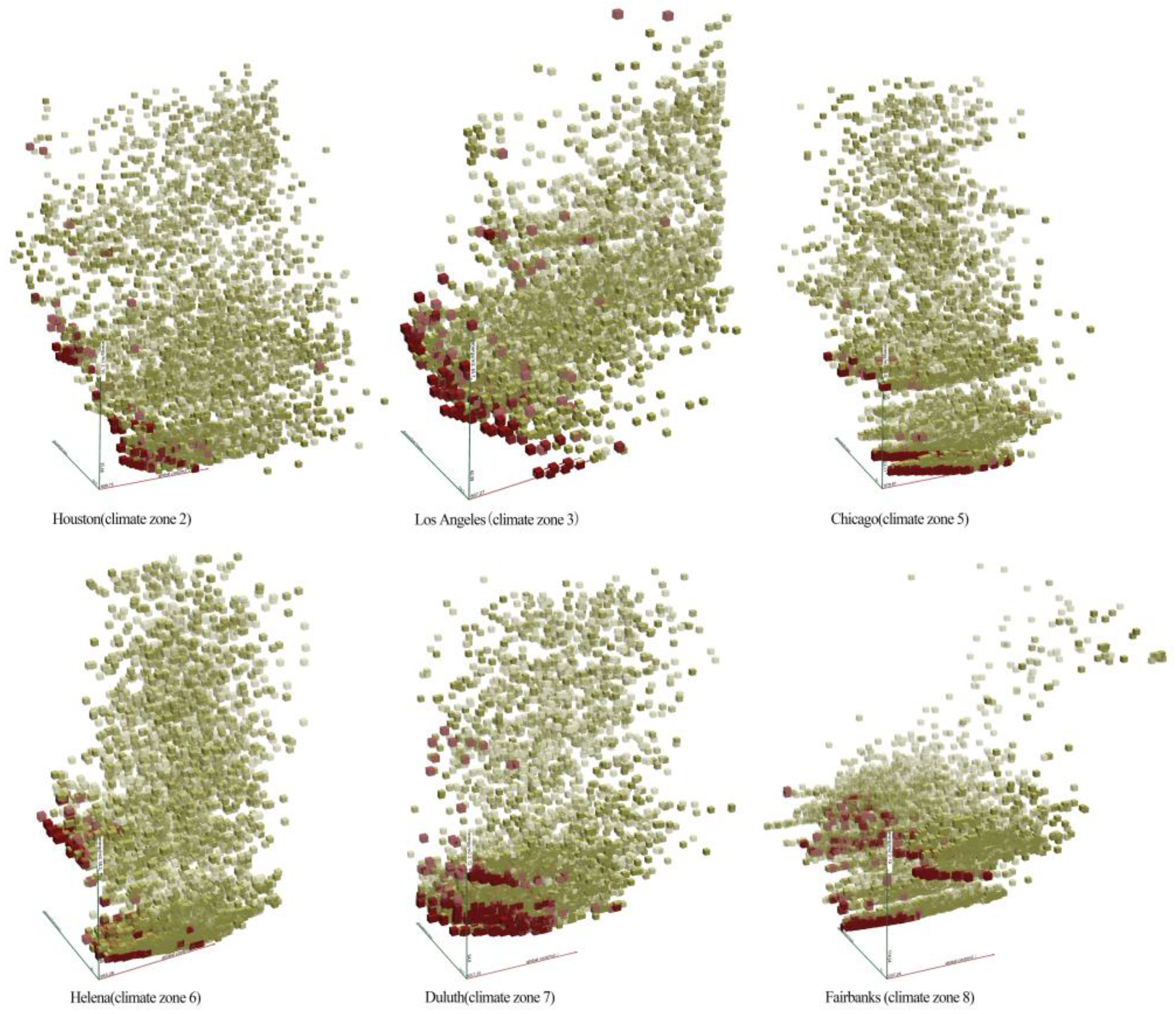
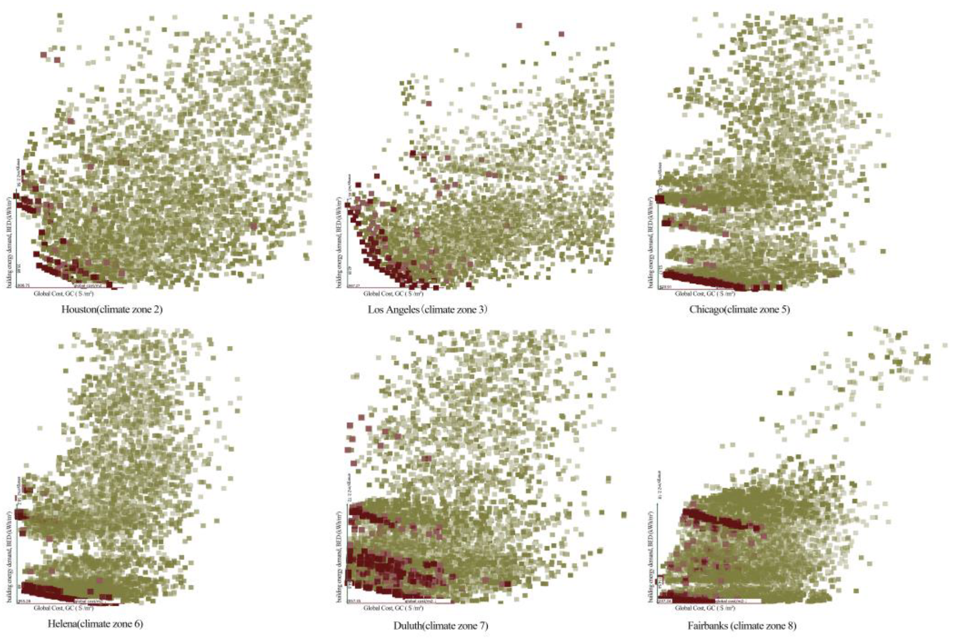
Figure 14 shows the optimization results of different climatic zones. In the three-dimensional space, all of Pareto non-dominated solutions with BED (building energy demand), GC (global cost), and DH (discomfort hour percentage) as objective functions are generated. These solutions represent trade-offs in design, because no other solution can improve (i.e., reduce) these three objectives at the same time. In order to better describe the optimization parameters, the three-dimensional solution is projected on the two-dimensional plane BED (horizontal axis)-GC (vertical axis) in Figure 15.
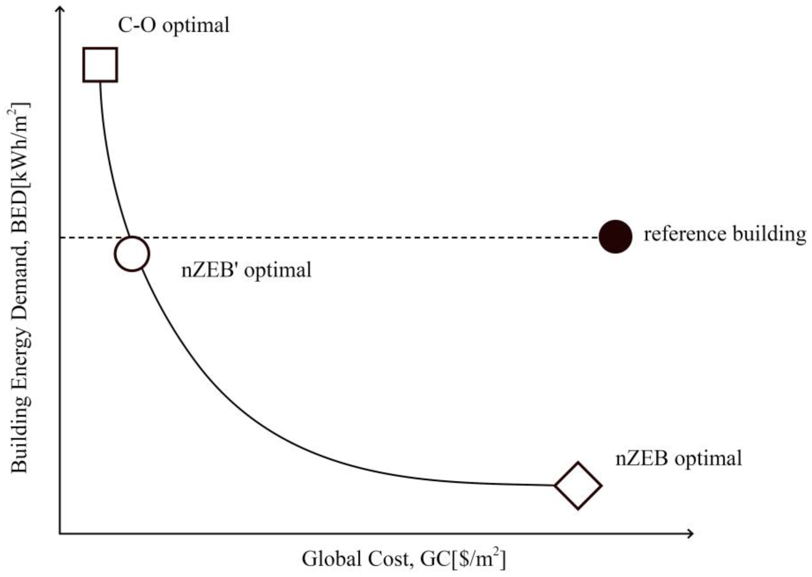
The study provides two optimal solutions, namely the energy-saving optimal solution (nZEB optimal) that minimizes building energy demand and the cost optimal solution (C-O optimal solution) that minimizes global costs. These two optimal solutions correspond to two different goals of public demand and private demand. In general, the main goal of the public social sector is to vigorously reduce energy consumption and pollution emissions, while the goal of private households is mainly to save costs and achieve indoor thermal comfort. Therefore, in Figure 14. BED-GC non-dominated solutions focus on analyzing the minimization of BED and GC. These solutions are part of the 3D non-dominated solution because there is no other solution to improve (i.e., reduce) BED and GC at the same time. Through the BED-GC Pareto Frontier, it is easy to know:
-
“Energy-saving optimal (nZEB) solution,” that is, BED is minimized in all non-dominated solutions, located at the right end of the 2D Pareto frontier of Figure 15. Although this solution is expressed as nZEB, it does not mean it meets the specific nZEB standard, but because this solution is a non-dominant solution with the lowest energy demand, and its performance is closest to the nZEB standard.
-
“Cost optimal (C-O) solution,” that is, the GC is minimized among all non-dominated solutions, located at the left end of the 2D Pareto frontier of Figure 15.
-
”nZEB’ solution,” when neither “energy-saving optimal (nZEB) solution” and “cost optimal (CO) solution” can meet the requirements of comprehensive indicators, in order to obtain a compromise result, it is necessary to introduce “nZEB’ Solution,” compared to the reference design, “nZEB’ solution” has lower GC and BED values (see Figure 16).
When the Pareto front in Figure 15 moves from left to right, the cost-effectiveness of the non-dominated solution gradually deteriorates, but the energy-saving effect gradually improves. Table 12, Table 13 and Table 14 list the optimized values of the design parameters and corresponding performance indicators, specifically, Table 12 lists the optimized values of the design parameters for each city in different climate zones, and Table 13 lists the corresponding building envelope heating transmittance (U value), Table 14 lists the performance indicator of the objective function under the optimized parameters and the investment cost.
From the analysis of the optimal objective function value in Table 14, it can be seen that except Los Angeles, from warm climate zone to cold climate zone, the BED value gradually increases, because in the calculation of energy demand, heating demand is higher than cooling demand. Specifically, in nZEB optimal solution, BED in Houston is 36.20 kWh/m2, GC is 286.97 $/m2, DH is 29.17%, whereas in Fairbanks, BED is 114.54 kWh/m2, GC is 418.76 $/m2, DH is 53.33%. In C-O optimal solution, BED in Houston is 53.45 kWh/m2, GC is 256.26 $/m2, DH is 41.67%, whereas in Fairbanks, BED is 162.55 kWh/m2, GC is 347.76 $/m2, DH is 61.67%. Whereas in Los Angeles, because of its climate characteristic, the energy demand is relatively lower than other cities.
According to nZEB and C-O optimal solutions, Table 12 lists the design parameters of residential buildings in different climate zones. In all optimization schemes, the best building orientation is the east–west orientation (0°), in order to facilitate the building to make maximum use of solar radiation in the colder season. As far as the optimization of the envelope parameters is concerned, the solar absorbance of the roof and external wall gradually increases from the warmer climate zone to the colder climate zone to maximize the utilization of solar radiation. For example, the solar absorbance of the roof and external wall in Houston residential building that is located in the south of the United States, is between 0.1 and 0.2, while that in Duluth and Fairbanks which are in the north of the United States are between 0.75 and 0.9.
The change in the thickness of envelope insulation is also related to the latitude of the city. The optimal solution for the US climatic zone 2 and climatic zone 3 represented by Houston and Los Angeles respectively does not recommend the use of insulation layers on roofs, external walls, and ground floors because these cities are in the southern United States. Compared with thermal insulation, it pays more attention to heat dissipation in summer. Therefore, the nZEB optimal solution in Houston and Los Angeles recommends the use of bricks with larger heat capacity on the building envelope. The thermal conductivity and density of the roof and ground floor bricks are 0.72 W/mK and 1800 Kg/m3, 0.9 W/mK, and 2000 Kg/m3 in Houston. The thermal conductivity and density of the external wall and ground floor bricks are 0.9 W/mK and 2000 Kg/m3, while for roof are 0.72 W/mK and 1800 Kg/m3 in Los Angeles. This helps the building absorb solar radiation during the day and delay solar energy entering the room, then at night when these heat-capacity materials release the solar energy absorbed during the day, heat is taken out of the room through night ventilation. With the exception of Houston and Los Angeles, the recommended values for the insulation thickness of external walls, roofs, and ground floors of the nZEB optimal for residential buildings in almost all cities are 0.12 m. The C-O optimal is quite different. Specifically, the thickness of the insulation layer on the external wall, roof and ground floor of the residential building in Chicago is 0.03 m, 0.04 m, and 0.03 m, respectively, making the U value of envelope slightly higher than that in the nZEB optimal, and the uncomfortable hours throughout the year is higher. In the Duluth C-O optimal solution, the thickness of the insulation layer of the external wall and roof is slightly lower than that of the nZEB optimal solution, which is 0.08 m and 0.1 m, respectively. But the block thermal conductivity and density of the roof and the ground floor in the C-O optimal solution are lower than the values in the nZEB optimal solution, which compensates for the lower thickness of the external wall and roof insulation layer, making the C-O optimal solution’s building energy demand value (BED) and the annual discomfort hours (DH) is not much different from that in the nZEB optimal solution, and reduces the global cost (GC) to some extent. In the Fairbanks C-O optimal solution, the recommended value of the insulation layer thickness of the external wall is 0.04 m, but the block thermal conductivity and density of the roof, external wall, and the ground floor of the C-O optimal solution and the nZEB optimal solution are the same, making the BED and DH values of the C-O optimal solution much higher than that in the nZEB optimal solution. Thus, a compromised nZEB’ solution is proposed, which uses the same insulation thickness of the roof, external wall, and ground floor, while only reducing the block thickness of roof and ground floor. The results show that the nZEB’ solution is able to achieve lower BED and DH values while reducing the global cost (GC), therefore, from the perspective of comprehensive indicators, it has better benefits. In general, when a thick insulation layer is installed in the envelope, the U value of it generally remains at a low value, between 0.15–0.18 W/m2K, when the insulation is not used, the U value of envelope is related to block thickness, thermal conductivity, and density. For example, the nZEB optimal solution and the C-O optimal solution in Houston are not recommended to install insulation on the external walls, roofs, and ground floors, however, the thermal conductivity and density of the roof and ground floor recommended by the C-O optimal solution are much lower than the nZEB optimal solution, leading to the U value of roof and ground floor in C-O optimal solution (0.87 W/m2K and 0.71 W/m2K) much lower than that in nZEB optimal solution (2.04 W/m2K and 1.45 W/m2K).
It can also be seen from the nZEB optimal solution that the block thickness of the external walls, roofs and ground floors gradually increases from the warmer climate zone to the colder climate zone. For example, the block thickness of the external wall and roof of residential buildings in Houston is 0.3 m and 0.25 m. In Los Angeles, the block thickness of that are 0.25 m, and ground floor is 0.4 m. The remaining cities are 0.4 m, while the block thickness of ground floor in Houston, Chicago, and Helena is 0.25 m, and that in Duluth and Fairbanks is 0.3 m. In addition, except Houston, Los Angeles, and Helena, the block thermal conductivity and density of the external wall and roof of residential buildings in various cities are always maintained between 0.25~0.3 W/mK and 600~800 kg/m3. For example, the block thermal conductivity and density for the roof of residential buildings in Houston and Helena are 0.72 W/mK, 1800 kg/m3, and 0.36 W/mK, 1000 kg/m3 respectively. In Los Angeles, the block thermal conductivity and density for the roof are 0.72 W/mK, 1800 kg/m3, and for external wall and ground floor are 0.9 W/mK, 2000 kg/m3. It is clear to see that the block thermal conductivity and density are gradually decreasing from south to north. For example, the thermal conductivity and density of ground floor in Houston and Chicago residential buildings are both 0.9 W/mK and 2000 kg/m3, while the corresponding values of Helena and Fairbanks residential buildings are 0.43 W/mK, 1200 kg/m3 and 0.25 W/mK, 600 kg/m3 respectively. It can be seen from the C-O optimal solution that the envelope block thermal conductivity and density in most typical cities’ residential buildings remained between 0.25 ~ 0.3 W/mK and 600 ~ 800 kg/m3.
For the transparent component of the envelope (i.e., windows), the triple-glazed with argon-filling, low-e coating, PVC frame window types are more common (i.e., type 7), for example, Chicago, Helena, Duluth, and Fairbanks nZEB optimal solution, Duluth C-O optimal solution, and Fairbanks nZEB’ optimal solution, although the price of this type of window is slightly high, but it has the best insulation performance. Houston’s nZEB optimal solution recommends the use of tinted double-glazed with argon-filling, low-e coating, PVC frame window (i.e., type 5), and the C-O optimal solution recommends the use of tinted double-glazed with air-filling, low-e coating, PVC frame window (i.e., type 2), this type of window has a low SHGC value of 0.38, which can effectively reduce excessive solar radiation entering the room. In Los Angeles, double-glazed with air-filling, low-e coating, aluminum frame window (type 1) is recommended in both nZEB optimal solution and C-O optimal solution, probably because it has the lowest price and will not increase the energy demand too much. Chicago, Helena, and Fairbanks C-O optimal solutions recommend double-glazed with argon-filling, low-e coating, PVC frame window (i.e., type 4). This type of window is cheaper and has a higher U value than other alternatives, which is 1.90 W/m2K, and the window SHGC is also high, which is 0.69, thus it can make better use of solar radiation, thereby greatly reducing the space heating energy.

4.2. Comparison of Optimization Results with Reference Buildings

Finally, the proposed optimal solution is compared with the climate-related reference design defined in the previous Table 11 and Table 15 shows the differences between BED, GC, IC, and DH.
In Houston, compared to the reference design, the BED of the nZEB optimal solution is reduced by approximately 20.55 kWh/m2, the global cost GC is reduced by approximately 36.55 $/m2, the initial investment cost is reduced by 25.22 $/m2, and the DH is reduced by 29.16%. In the CO optimal solution, although the value of GC decreased significantly, it was 67.26 $/m2, which was due to the low initial investment, which reduced to 65.4 $/m2; but the reduction in BED was very small, only 3.3 kWh/ m2, and the reduction of DH is not as effective as the nZEB program, which is 16.66% less than the reference building, making the uncomfortable hours of the year still 41.67%, so the applicability of this program in actual practice is not as good as nZEB optimal solution.
In Los Angeles, the energy demand of the reference building is very low, which is only 7.28 kWh/m2, thus the nZEB optimal solution cannot improve it a lot. From the Table 15, it can be seen that the BED in nZEB optimal solution is only improved by 5.24 kWh/m2, but DH is increased by 45.84%, meanwhile the IC is also increased by 13.7 $/m2. Compared with nZEB optimal solution, the C-O optimal solution decreases the GC by 92.98 $/m2 and IC by 91.71 $/m2, while only increasing DH by 8.34%. Therefore, in this climate zone, C-O optimal solution is more practical than nZEB optimal solution.
Compared with the reference design, the climate zone 5 represented by Chicago has reduced the BED in the nZEB optimal solution by approximately 20.45 kWh/m2 and DH by 13.17%, but increased the global cost by a small amount, the GC increased by approximately 14.71 $/m2, which is due to an increase in IC of approximately 25.94 $/m2. Compared with nZEB optimal, CO optimal greatly reduced the GC about 79.68 $/m2 and the IC about 82.54 $/m2, but at the expense of building energy demand and thermal environment comfort. Specifically, BED increased by 5.21 kWh/m2, DH remains the same as the reference building in 59.17%, thus compared to the C-O optimal solution, the nZEB optimal solution is more suitable for facilitating the actual design.
In the climate zone 6 represented by Helena, although the nZEB optimal solution has reduced BED by 22.32 kWh/m2 and DH by 12.5%, the cost has increased by 61.99 $/m2, which is due to the increase in IC (74.64 $/m2). The CO optimal solution reduces the building energy demand and improves the indoor thermal environment comfort, meanwhile, it also reduces the global investment cost. Specifically, BED is reduced by 18.8 kWh/m2, DH is reduced by 8.34%, GC and IC are reduced by 13.81 $/m2 and 6.27 $/m2, respectively. Therefore, the design parameters of the C-O optimal solution can be used as reference values for energy-saving design of residential buildings in climate zone 5 cities such as Chicago.
In Duluth, compared to the reference building, the BED in the nZEB optimal solution decreased by approximately 28.32 kWh/m2, and the DH decreased by 8.75%, but the GC and IC increased 28.71 $/m2 and 44.24 $/m2 respectively. Compared with the nZEB optimal solution, the GC and IC optimization of the C-O optimal solution did not come at the expense of the degradation of BED and DH. In the C-O optimal solution, BED decreased by approximately 20.43 kWh/m2, DH decreased by 6.25%, GC and IC decreased by 38.68 $/m2 and 27.47 $/m2, respectively. Therefore, from the perspective of comprehensive indicators, the design parameters of the C-O optimal solution can be used as the reference value for energy-saving design of residential buildings in Duluth.
In the climate zone 8 represented by Fairbanks, the BED of the nZEB optimal solution decreased by approximately 55.23 kWh/m2, the GC decreased by 56.97 $/m2, the IC decreased by 26.65 $/m2, and the DH decreased by 8.97%. Whereas in the C-O optimal solution, BED only decreased by about 7.22 kWh/m2, GC decreased by 127.97 $/m2, IC decreased by 106.12 $/m2, and DH decreased by 0.63%. From the aspects of building energy demand and global cost, the improvement of these two optimal solutions are not large, so a compromise nZEB’ optimal solution is proposed. In the nZEB’ optimal solution, BED is reduced by 52.37 kWh/m2, GC is reduced by 111.66 $/m2, IC is reduced by 82.91 $/m2, DH is reduced by 14.05%, the comprehensive indicator is better than nZEB optimal solution and CO optimal solution, thus it can be used as a reference value for residential buildings energy efficiency design in Fairbanks.
As can be seen from the comparison of different optimal solutions with reference buildings, the optimal design reference value of some typical cities in the United States can take the recommended value of the nZEB optimal solution, such as Houston and Chicago, because the nZEB optimal solution of these cities is superior to the CO optimal solution. While the optimal design parameters of Los Angeles, Helena and Duluth should take the recommended value of the C-O optimal solution, because in the C-O optimal solution, the best GC are able to be achieved without increasing BED, from an economic point of view, it is more suitable as an actual project reference value. Unlike the above cities, the optimal design parameters of Fairbanks should refer to the recommended value of nZEB’, because the comprehensive index of the nZEB’ solution is better than the nZEB optimal solution and the C-O optimal solution.
It can be seen from the comparison between the optimized design results and the reference building design that the best solution provides different guidelines for the energy-saving design of residential buildings in typical cities in the United States. Mainly as follows:
  • The best building orientation is 0°, i.e., from east to west;
  • In terms of external wall energy-saving design parameters, the solar absorbance of the external wall of residential buildings in the warm climate zone (Houston) can be lower (0.1), while cities in the colder climate zone require a higher solar absorbance. Besides, if the wall uses insulation in a typical city other than Houston and Los Angeles, the optimal thickness should be 0.10–0.12 m, much higher than that in the reference building (the reference building insulation thickness is 0.03–0.05 m). Moreover, the external wall is recommended to use low density and low thermal conductivity materials.
  • Similar to the external wall, the solar absorbance of the roof of residential buildings in the warm climate zone (Houston) can be lower (0.1), and that in the cold climate zone should be higher, the best roof insulation thickness should be 0.10–0.12 m which are similar to the reference buildings. It is recommended to use high thermal mass materials for roofs in warm climate zones, and low thermal mass materials for roofs in cold climate zones.
  • The ground floor is different from the external walls and roofs, as there is no direct solar radiation, the solar absorbance ranges are not predefined. However, the optimal insulation thickness of the ground floor in colder areas (except Houston and Los Angeles) should be 0.10–0.12 m, which is higher than that of the reference buildings (0.03–0.06 m), while residential buildings in Houston and other warmer areas are not recommended to use insulation, but it is recommended to use high thermal mass materials.
  • For windows, some cities (such as Chicago, Duluth, and Fairbanks) reference buildings that are filled with double-glazed argon-filling, low-e coating, PVC frame windows (type 4) can be replaced with triple-glazed with argon-filling, low-e coating, PVC frame windows (type 7).

5. Conclusions

The study selected six typical cities based on the climate zoning in the United States, established an optimization process using Octopus based on the Grasshopper parametric platform, and made multi-objective optimization decisions on the residential building model, including building energy demand, annual discomfort hours, and global cost. Through the Pareto front, the design parameters suitable for typical urban residential buildings are obtained. The study compares the optimal design parameters of each typical city with the reference building parameters recommended by the local energy conservation codes to quantify to what extent the optimal design improves the performance of typical urban residential buildings under various climatic conditions.
In addition, this research also draws the following conclusions:
(1)
For low energy demand and high thermal comfort passive buildings, it is possible to create good environmental benefits while meeting economic requirements. Therefore, it is necessary to optimize different objectives in the schematic stage and control the building design from the initial stage.
(2)
The optimal solution set obtained through the passive energy-saving technology screening can be divided into two types of selection templates: energy-saving optimal (nZEB optimal) and global cost optimal (C-O optimal) according to different priorities. Meanwhile, the design parameter interval of the trade-off optimal solution (nZEB’) can be searched according to the existing performance of the reference building.
(3)
The multi-objective optimization framework based on the typical residential building model, using the meteorological data of typical cities in different climatic regions, can derive the optimal design parameters for residential buildings in different climatic zones. Comparing the performance of the optimal design with the reference models of residential buildings in different climatic regions, climate responsive design strategy can be proposed for local residential buildings from the perspective of two stakeholders, the public sector and private residents, to achieve energy-efficient development of residential buildings.

Author Contributions

In this paper, Z.L. performed the experiment, including conceptualization, simulation, calculation and data visualization, P.V.G. supervised and reviewed the paper. Y.Z., data handling and reviewed the paper. All the authors (Z.L., P.V.G., and Y.Z.) organized the paper structure. All authors have read and agreed to the published version of the manuscript.

Funding

This research received no external funding.

Conflicts of Interest

The authors declare no conflict of interest.

References

  1. Givoni, B. Man, Climate and Architecture; Applied Science Publishers Ltd.: London, UK, 1969. [Google Scholar]
  2. Alsousi, M. User Response to Energy Conservation and Thermal Comfort of High-Rise Residential Buildings in Hot Humid Region with Referring to Gaza. Ph.D. Thesis, University of Nottingham, Nottingham, UK, 2005. [Google Scholar]
  3. Ghisi, E.; Massignani, R.F. Thermal performance of bedrooms in a multi-storey residential building in southern Brazil. Build. Environ. 2007, 42, 730–742. [Google Scholar] [CrossRef]
  4. Lartigue, B.; Lasternas, B.; Loftness, V. Multi-objective optimization of building envelope for energy consumption and daylight. Indoor Built Environ. 2014, 23, 70–80. [Google Scholar] [CrossRef]
  5. Wright, J.; Loosemore, H.; Farmani, R. Optimization of building thermal design and control by multi-criterion genetic algorithm. Energy Build. 2002, 34, 959–972. [Google Scholar] [CrossRef]
  6. Ciancio, V.; Salata, F.; Falasca, S.; Curci, G.; Golasi, I.; de Wilde, P. Energy demands of buildings in the framework of climate change: An investigation across Europe. Sustain. Cities Soc. 2020, 60, 102213. [Google Scholar] [CrossRef]
  7. Harkouss, F.; Fardoun, F.; Biwole, P.H. Passive design optimization of low energy buildings in different climates. Energy 2018, 165, 591–613. [Google Scholar] [CrossRef]
  8. Diakaki, C.; Grigoroudis, E.; Kabelis, N.; Kolokotsa, D.; Kalaitzakis, K.; Stavrakakis, G. A multi-objective decision model for the improvement of energy efficiency in buildings. Energy 2010, 35, 5483–5496. [Google Scholar] [CrossRef]
  9. Wang, W.; Zmeureanu, R.; Rivard, H. Applying multi-objective genetic algorithms in green building design optimization. Build. Environ. 2005, 40, 1512–1525. [Google Scholar] [CrossRef]
  10. Bakar, N.N.A.; Hassan, M.Y.; Abdullah, H.; Rahman, H.A.; Abdullah, M.P.; Hussin, F.; Bandi, M. Energy efficiency index as an indicator for measuring building energy performance: A review. Renew. Sustain. Energy Rev. 2015, 44, 1–11. [Google Scholar] [CrossRef]
  11. Lam, J.C.; Wan, K.K.W.; Liu, D.; Tsang, C.L. Multiple regression models for energy use in air-conditioned office buildings in different climates. Energy Convers. Manag. 2010, 51, 2692–2697. [Google Scholar] [CrossRef]
  12. Asadi, E.; da Silva, M.G.; Antunes, C.H.; Dias, L. A multi-objective optimization model for building retrofit strategies using TRNSYS simulations, GenOpt and MATLAB. Build. Environ. 2012, 56, 370–378. [Google Scholar] [CrossRef]
  13. Asl, M.R.; Zarrinmehr, S.; Bergin, M.; Yan, W. BpOp: A framework for BIM-based performance optimization. Energy Build. 2015, 108, 401–412. [Google Scholar]
  14. Pernigotto, G.; Penna, P.; Cappelletti, F.; Gasparella, A. Extensive utilization of dynamic simulation for sensitivity analysis and optimization design of refurbishment measures. In Proceedings of the II International High Performance Buildings Conference, Purdue, IN, USA, 16–19 July 2012. [Google Scholar]
  15. Echenagucia, T.M.; Capozzoli, A.; Cascone, Y.; Sassone, M. The early design stage of a building envelope: Multi-objective search through heating, cooling and lighting energy performance analysis. Appl. Energy 2015, 154, 577–591. [Google Scholar] [CrossRef]
  16. Prada, A.; Pernigotto, G.; Cappelletti, F.; Gasparella, A.; Jan, L.M. HENSEN. Robustness of multi-objective optimization of building refurbishment to suboptimal weather data. In Proceedings of the International High Performance Building Conference, Purdue, IN, USA, 14–17 July 2014. [Google Scholar]
  17. Pernigotto, G.; Prada, A.; Cappelletti, F.; Gasparella, A. Impact of reference years on the outcome of multi-objective optimization for building energy refurbishment. Energies 2017, 10, 1925. [Google Scholar] [CrossRef] [Green Version]
  18. Penna, P.; Prada, A.; Cappelletti, F.; Gasparella, A. Multi-objectives optimization of energy efficiency measures in existing buildings. Energy Build. 2015, 95, 57–69. [Google Scholar] [CrossRef]
  19. Chen, J.; Augenbroe, G.; Song, X. Evaluating the potential of hybrid ventilation for small to medium sized office buildings with different intelligent controls and uncertainties in USA climates. Energy Build. 2018, 158, 1648–1661. [Google Scholar] [CrossRef]
  20. Yong, S.; Kim, J.H.; Gim, Y.; Kim, J.; Cho, J.; Hong, H.; Baik, Y.; Koo, J. Impacts of building envelope design factors upon energy loads and their optimization in USA standard climate zones using experimental design. Energy Build. 2017, 141, 1–15. [Google Scholar] [CrossRef]
  21. IECC. International Code Council. 2018. Available online: https://www.iccsafe.org/wp-content/uploads/01-Prelims1.pdf (accessed on 15 August 2020).
  22. Zitzler, E.; Laumanns, M.; Thiele, L. SPEA2: Improving the strength pareto evolutionary algorithm for multiobjective optimization[C]. In Evolutionary Methods for Design, Optimization and Control with Applications to Industrial Problems; EUROGEN: Athens, Greece, 2001. [Google Scholar]
  23. Corne, D.W.; Jerram, N.R.; Knowles, J.D.; Oates, M.J. PESA-II: Region-based selection in evolutionary multi-objective optimization[C]. In Proceedings of the Genetic and Evolutionary Computation Conference GECCO; Sbedtor, L., Goodman, E.D., Wu, A., Langdon, W.B., Voigt, H.M., Gen, M., Eds.; Morgan Kaufmann Publishers: San Francisco, CA, USA, 2001; pp. 283–290. [Google Scholar]
  24. ANSI/ASHRAE. Standard 55: Thermal Environmental Conditions for Human Occupancy. 2013. Available online: https://www.ashrae.org/technical-resources/bookstore/standard-55-thermal-environmental-conditions-for-human-occupancy (accessed on 15 August 2020).
  25. ASHRAE. Handbook Fundamentals; American Society of Heating Refrigerating and Air-Conditioning Engineers: Atlanta, GA, USA, 2009. [Google Scholar]
  26. Pedersen, C.O.; Fisher, D.E.; Liesen, R.J. Development of a heat balance procedure for calculating cooling loads. ASHRAE Trans. 1997, 103, 459–468. [Google Scholar]
  27. Walton, G.N. Thermal Analysis Research Program Reference Manual; National Bureau of Standards: Gaithersburg, MD, USA, 1983.
  28. O’Neill, Z.; Eisenhower, B. Leveraging the analysis of parametric uncertainty for building energy model calibration. Build. Simulat. 2013, 6, 365–377. [Google Scholar] [CrossRef]
  29. European Committee for Standardization CEN/TR 15615: Explanation of the General Relationship between Various European Standards and the Energy Performance of Building Directive (EBPD); Umbrella Document; European Committee for Standardization (CEN): Tallinn, Estonia, 2008; Available online: https://standards.iteh.ai/catalog/standards/cen/d7208116-9623-4117-8d99-4c81230c6f5e/cen-tr-15615-2008 (accessed on 15 August 2020).
  30. EN 15459: Energy Performance of Buildings. Economic Evaluation Procedure for Energy Systems in Buildings. 2007. Available online: https://standards.iteh.ai/catalog/standards/cen/ff0c5a0e-d363-40ab-80b3-7d7cc28b19a5/en-15459-1-2017 (accessed on 15 August 2020).
  31. Ferrara, M.; Monetti, V.; Fabrizio, E. Cost-optimal analysis for nearly zero energy buildings design and optimization: A critical review. Energies 2018, 11, 1478. [Google Scholar] [CrossRef] [Green Version]
  32. Ascione, F.; Bianco, N.; De Masi, R.F.; Mauro, G.M.; Vanoli, G.P. Resilience of robust cost-optimal energy retrofit of buildings to global warming: A multi-stage, multi-objective approach. Energy Build 2017, 153, 150–167. [Google Scholar] [CrossRef]
  33. Ascione, F.; Bianco, N.; Mauro, G.M.; Napolitano, D.F. Building envelope design: Multi-objective optimization to minimize energy consumption, global cost and thermal discomfort. Application different Italian climatic zones. Energy 2019, 174, 359–374. [Google Scholar] [CrossRef]
Figure 1. (a): divergent and convergent stage; (b): repetition of divergence and convergence; (c): scenario exploration process.
Algorithms 13 00238 g001
Figure 2. Deterministic forward simulation (a), probabilistic forward modeling (b), probabilistic reverse simulation workflow (c).
Algorithms 13 00238 g002
Figure 3. U.S. climatic zoning map [20].
Algorithms 13 00238 g003
Figure 4. Location of typical cities in the United States.
Algorithms 13 00238 g004
Figure 5. Basic steps of design generation and optimization.
Algorithms 13 00238 g005
Figure 6. Simulation based modeling and optimization process.
Algorithms 13 00238 g006
Figure 7. Parametric building optimization process.
Algorithms 13 00238 g007
Figure 8. SPEA-II work flow.
Algorithms 13 00238 g008
Figure 9. Diagram of SPEA-II algorithm work flow.
Algorithms 13 00238 g009
Figure 10. Environmental selection process.
Algorithms 13 00238 g010
Figure 11. Typical models for optimization.
Algorithms 13 00238 g011
Figure 12. Grasshopper operation process.
Algorithms 13 00238 g012
Figure 13. Multi-objective optimization iteration with Duluth as an example.
Algorithms 13 00238 g013
Figure 14. Pareto optimization frontiers of typical cities in the United States.
Algorithms 13 00238 g014
Figure 15. Building energy demand (BED, vertical axis) and global cost (GC, horizontal axis) Pareto frontier in typical American cities.
Algorithms 13 00238 g015
Figure 16. Relationship between nZEB, nZEB’, and C-O optimal solutions.
Algorithms 13 00238 g016
Table 1. Heating period in US typical cities [21].
Climate ZoneTypical CitiesHeating/Cooling Degree DaysHeating Period (Day/Month)Heating Hours of Each Day
2Houston3500 < CDD (10 °C) ≤ 5000No mandatory requirement-
3Los Angeles2500 < CDD (10 °C) ≤ 3500 HDD (18 °C) ≤ 3000No mandatory requirement-
5Chicago3000 < HDD (18 °C) ≤ 400015/9–1/614 h
6Helena4000 < HDD (18 °C) ≤ 50001/10–1/524 h
7Duluth5000 < HDD (18 °C) ≤ 700015/10–15/424 h
8Fairbanks7000 < HDD (18 °C)No restrictions24 h
Table 2. Input parameters for thermal comfort calculation.
MonthOutdoor TemperatureIndoor Air SpeedClothing Thermal ResistanceMetabolic Rate
(°C)(m/s)(CLO)(met)
12.150.051.11.2
21.660.051.11.2
36.510.050.91.2
413.210.050.81.2
516.320.050.61.2
620.870.050.51.2
724.810.050.41.2
823.260.050.51.2
919.020.050.61.2
1014.720.050.71.2
118.490.050.91.2
123.090.051.11.2
Table 3. Parameters of typical model.
TypeSub-CategoryParameter CategoryUnitData Range
LocationClimateClimatic parameters of typical cities-According to meteorological parameters of typical cities
Building geometryBuilding typeNumber of floors-2.00
Net height of each floorm2.70
Gross height of each floorm3.10
Length (S/N direction)m7.9
Aspect ratio-2
Window to wall ratio (WWR)-0.15
orientationdeg0
Geometric parametersVolume774
Total surface area544
Total floor area250
Surface to volume ratio-0.7
Envelope design parametersEnvelopeU value external wallsW/(m2K)According to Table 9
U value ground floorW/(m2K)
U value roofW/(m2K)
U value transparent componentsW/(m2K)
SHGC factor glass-
Building operation parametersActivitiesInternal gains (lighting, appliances and occupancy, daily average)W/m25
Control and operation settingHeating set-point temperature°C20
Cooling set-point temperature°C26
Air-change rate (infiltration and natural ventilation)vol/h0.8
ScheduleN.Adjustment according to different cities requirements
Table 4. Material parameters of building envelope.
Ground Floor
LayersMaterialThicknessThermal ConductivityDensitySpecific Heat (°C)Thermal ResistanceHeat Absorption RateSolar AbsorptivityVisible Absorbance
(m)(W/mK)(kg/m3)(J/kgK)(m2K/W)(-)(-)(-)
1Ceramic mortar0.0301.1620008800.0260.9000.7000.700
2Polyurethane board0.040.0257014641.6000.9000.7000.700
3Concrete floor slab0.061.3022008800.0460.9000.7000.700
4Pebble0.1500.7017008400.2140.9000.7000.700
Internal floor and ceiling
1Ceramic tile0.011.0023008000.0100.9000.7000.700
2Ceramic mortar0.030.8020008800.0380.9000.7000.700
3Lightweight expansive clay aggregate0.050.125008800.4170.9000.7000.700
4Mortar for hollow bricks0.041.3022008800.0310.9000.7000.700
5Hollow brick slab0.160.482508800.3300.9000.7000.700
6plaster0.010.60140010100.0170.9000.3000.300
External wall
1plaster0.0150.60140010100.0250.9000.3000.300
2Hollow brick0.080.40018008400.2000.9000.8000.800
3Polyurethane board0.040.0257014641.6000.9000.7000.700
4lime0.0100.60014008800.0170.9000.7000.700
5Hollow brick0.1200.40018008400.3000.9000.8000.800
6plaster0.0150.90018009100.0170.9000.3000.300
roof
1Brick board0.1600.802508800.2000.8500.6500.650
2Polyurethane board0.040.0257014641.6000.9000.7000.700
Table 5. Design parameters for reference buildings in each climate zone.
NDesign VariableParameter
1Building orientation (°)−45; 0; 45
2Solar absorbance of external wall (-)0.1; 0.25; 0.4; 0.5; 0.6; 0.7; 0.8; 0.9
3Solar absorbance of roof (-)0.1; 0.2; 0.3; 0.4; 0.5; 0.6; 0.75; 0.9
4Insulation thickness of external wall (m)0; 0.03; 0.04; 0.05; 0.06; 0.08; 0.10; 0.12
5Insulation thickness of roof (m)0; 0.03; 0.04; 0.05; 0.06; 0.08; 0.10; 0.12
6Insulation thickness of ground floor (m)0; 0.03; 0.04; 0.05; 0.06; 0.08; 0.10; 0.12
7Block thickness for external wall (m)0.25; 0.30; 0.35; 0.40
8Block thermal conductivity for the external wall (W/mK) *0.25; 0.30; 0.36; 0.43; 0.50; 0.59; 0.72; 0.90
Block density for the external wall (Kg/m3) *600; 800; 1000; 1200; 1400; 1600; 1800; 2000
9Block thickness for roof (m)0.25; 0.30; 0.35; 0.40
10Block thermal conductivity for the roof (W/mK) *0.25; 0.30; 0.36; 0.43; 0.50; 0.59; 0.72; 0.90
Block density for the roof (Kg/m3) *600; 800; 1000; 1200; 1400; 1600; 1800; 2000
11Block thickness for ground floor (m)0.25; 0.30; 0.35; 0.40
12Block thermal conductivity for the ground floor (W/mK) *0.25; 0.30; 0.36; 0.43; 0.50; 0.59; 0.72; 0.90
Block density for the ground floor (Kg/m3) *600; 800; 1000; 1200; 1400; 1600; 1800; 2000
13Types of window (see Table 6)1; 2; 3; 4; 5; 6; 7 (see Table 6)
(*) To each value of thermal conductivity corresponds the respective value of density (e.g., to the first value of conductivity corresponds the first value of density, and so on).
Table 6. Different types of windows and their parameters and investment costs.
NTypeU (W/m2K)SHGC (-)Investment Cost ($/m2)
1Double-glazed with air-filling, low-e coating, aluminum frame3.090.69269.37
2Tinted double-glazed with air-filling, low-e coating, PVC frame1.950.38280.14
3Selective double-glazed with air-filling, low-e coating, PVC frame1.840.43280.14
4Double-glazed with argon-filling, low-e coating, PVC frame1.900.69280.14
5Tinted double-glazed with argon-filling, low-e coating, PVC frame1.720.37290.92
6Selective double-glazed with argon-filling, low-e coating, PVC frame1.590.43290.92
7Triple-glazed with argon-filling, low-e coating, PVC frame1.350.58312.46
Table 7. Calculation method of initial investment cost.
NDesign VariablesInvestment Cost (IC) [$]
1Building orientation (°)-
2Solar absorbance of the external wall (-)The plaster cost is taken into account in the cost of the related vertical walls or roof
3Solar absorbance of the roof (-)
4Insulation thickness of the external wall (m)Insulation cost:
I C = [ ( 500 2000 t ) t + 15 ] A
“A” indicates the frontal area of the building envelope component, “t” denotes the thickness of the insulation layer[32]
5Insulation thickness of the roof (m)
6Insulation thickness of the ground floor (m)
7Block thickness for the external wall (m)Block cost
I C = [ 224.65 + ( 329.9 224.65 ) ( p 600 ) ( 2000 600 ) ] A t b
“r” stands for the density of the block material
“A” indicates the frontal area of the building envelope component
“tb” denotes the thickness of the block material [33]
8Block thermal conductivity for the external wall (W/mK) *
Block density for the external wall (Kg/m3) *
9Block thickness for the roof (m)
10Block thermal conductivity for the roof (W/mK) *
Block density for the roof (Kg/m3) *
11Block thickness for the ground floor (m)
12Block thermal conductivity for the ground floor (W/mK) *
Block density for the ground floor (Kg/m3) *
13Type of windows (see Table 6)see Table 6
14Energy cost (annual heating and cooling demand)0.15 $/kWh
The * refers to the unified change of block thermal conductivity and block density in parametric simulation. For example, the block thermal conductivity of roof are consistently change with block density of roof. Same as external wall and ground floor control.
Table 8. Typical cities selected according to American climate zones.
CityHeating Degree Days (18 °C)Climate Zone
Houston620Climate zone 2
Los Angeles810Climate zone 3
Chicago3611Climate zone 5
Helena4395Climate zone 6
Duluth5642Climate zone 7
Fairbanks7215Climate zone 8
Table 9. U value of reference building envelopes in different typical cities of the United States.
U Value of Reference Building (W/m2K)Climate Zone 2Climate Zone 3Climate Zone 5Climate Zone 6Climate Zone 7Climate Zone 8
External wall0.6980.5910.4430.4030.3460.346
Roof0.2730.2730.2210.1820.1590.159
Ground floor0.4940.4320.3630.3240.2900.290
Window2.32.31.81.81.81.8
Table 10. Design parameters of reference buildings in various cities of the United States.
NDesign VariableClimate Zone 2Climate Zone 3Climate Zone 5Climate Zone 6Climate Zone 7Climate Zone 8
HoustonLos AngelesChicagoHelenaDuluthFairbanks
1Building orientation (°)000000
2Solar absorbance of external wall (-)0.10.40.50.40.80.8
3Solar absorbance of roof (-)0.10.30.50.60.750.75
4Insulation thickness of external wall (m)000.030.030.040.05
5Insulation thickness of roof (m)0.080.050.080.120.120.12
6Insulation thickness of ground floor (m)0.030.030.030.050.060.06
7Block thickness for external wall (m)0.250.350.30.30.30.4
8Block thermal conductivity for the external wall (W/mK) *0.250.250.50.360.360.9
Block density for the external wall (Kg/m3) *600600140080010002000
9Block thickness for roof (m)0.30.40.40.250.350.3
10Block thermal conductivity for the roof (W/mK) *0.90.250.360.430.250.25
Block density for the roof (Kg/m3) *200060010001200600600
11Block thickness for ground floor (m)0.30.40.350.250.40.35
12Block thermal conductivity for the ground floor (W/mK) *0.720.590.30.360.590.59
Block density for the ground floor (Kg/m3) *18001600800100016001600
13Types of window (see Table 6)114444
The * refers to the unified change of block thermal conductivity and block density in parametric simulation. For example, the block thermal conductivity of roof are consistently change with block density of roof. Same as external wall and ground floor control.
Table 11. Performance indicators for residential building design in typical cities of the United States.
Reference Building Performance IndicatorClimate Zone 2Climate Zone 3Climate Zone 5Climate Zone 6Climate Zone 7Climate Zone 8
HoustonLos AngelesChicagoHelenaDuluthFairbanks
BED (kWh/m2): Building Energy Demand56.757.2873.7872.0393.78169.77
GC ($/m2): Global Cost323.52322.63378.58335.89389.09475.73
DH (%): Discomfort Hours percentage58.338.3359.1741.6761.2562.30
IC ($/m2): Investment Cost292.32318.63338.08297.90337.62382.54
Table 12. Optimal design parameters for typical cities in each U.S climate zone.
NDesign VariableHoustonLos AngelesChicagoHelenaDuluthFairbanks
nZEB (*)C-O (*)nZEB (*)C-O (*)nZEB (*)C-O (*)nZEB (*)C-O (*)nZEB (*)C-O (*)nZEB (*)nZEB’ (*)C-O (*)
1Building orientation (°)0000000000000
2Solar absorbance of external wall (-)0.10.10.10.10.90.50.90.40.90.80.90.90.9
3Solar absorbance of roof (-)0.10.20.30.30.750.50.40.60.90.90.90.90.75
4Insulation thickness of external wall (m)00000.120.030.120.120.120.080.120.120.04
5Insulation thickness of roof (m)00000.120.040.120.120.120.10.120.120.12
6Insulation thickness of ground floor (m)000.0300.120.030.120.120.120.120.120.120.12
7Block thickness for external wall (m)0.30.250.250.250.40.250.40.250.40.30.40.250.25
8Block thermal conductivity for the external wall (W/mK) *0.30.250.90.250.250.250.360.250.30.30.250.250.25
Block density for the external wall (Kg/m3) *80060020006006006001000600800800600600600
9Block thickness for roof (m)0.250.250.250.250.40.250.40.250.40.250.40.250.25
10Block thermal conductivity for the roof (W/mK) *0.720.250.720.250.250.250.30.250.30.250.250.30.25
Block density for the roof (Kg/m3) *18006001800600600600800600800600600800600
11Block thickness for ground floor (m)0.250.250.40.250.250.250.250.250.30.250.30.250.25
12Block thermal conductivity for the ground floor (W/mK) *0.90.250.90.250.90.250.430.250.90.250.250.250.25
Block density for the ground floor (Kg/m3) *20006002000600200060012006002000600600600600
13Types of window (see Table 6)5211747477774
(*) nZEB: near zero energy building solution; nZEB’: constrained nearly zero energy building solution; C-O: cost optimal solution.
Table 13. Optimal U value of building envelope.
U Value (W/m2K)HoustonLos AngelesChicagoHelenaDuluthFairbanks
nZEB (*)C-O (*)nZEB (*)C-O (*)nZEB (*)C-O (*)nZEB (*)C-O (*)nZEB (*)C-O (*)nZEB (*)nZEB’ (*)C-O (*)
External wall0.610.701.410.700.150.380.160.160.150.220.150.160.33
Roof2.040.872.040.870.150.360.160.170.160.190.150.170.17
Ground floor1.450.711.160.710.180.380.170.160.180.160.160.160.16
Window1.721.951.951.951.351.91.351.901.351.351.351.351.90
(*) nZEB: near zero energy building solution; nZEB’: constrained nearly zero energy building solution; C-O: cost optimal solution.
Table 14. Performance indicator of optimal solution.
Performance IndicatorHoustonLos AngelesChicagoHelenaDuluthFairbanks
nZEB (*)C-O (*)nZEB (*)C-O (*)nZEB (*)C-O (*)nZEB (*)C-O (*)nZEB (*)C-O (*)nZEB (*)nZEB’ (*)C-O (*)
BED (kWh/m2): Building Energy Demand36.2053.452.044.9653.3378.9949.7158.2365.4673.35114.54117.40162.55
GC ($/m2): Global Cost286.97256.26306.06229.65393.29298.90397.88322.08417.80350.41418.76364.07347.76
DH [%]: Discomfort Hours percentage29.1741.6754.1716.674659.1729.1733.3352.55553.3348.2561.67
IC [$/m2]: Investment Cost267.10226.92304.93226.92364.02255.54372.54291.63381.86310.15355.89299.63276.42
(*) nZEB: near zero energy building solution; nZEB’: constrained nearly zero energy building solution; C-O: cost optimal solution.
Table 15. Comparison between the proposed optimal solutions and the related reference designs.
Performance IndicatorHoustonLos AngelesChicagoHelenaDuluthFairbanks
nZEB (*)C-O (*)nZEB (*)C-O (*)nZEB (*)C-O (*)nZEB (*)C-O (*)nZEB (*)C-O (*)nZEB (*)nZEB’ (*)C-O (*)
BED reduction (kWh/m2) (**)20.553.3−5.24−2.3220.45−5.2122.3218.828.3220.4355.2352.377.22
GC reduction ($/m2) (**)36.5567.26−16.57−92.98−14.7179.68−61.9913.81−28.7138.6856.97111.66127.97
DH reduction (%) (**)29.1616.6645.848.3413.17012.58.348.756.258.9714.050.63
IC reduction ($/m2) (**)25.2265.413.7−91.71−25.9482.54−74.646.27−44.2427.4726.6582.91106.12
(*) nZEB: near zero energy building solution; nZEB’: constrained nearly zero energy building solution; C-O: cost optimal solution. (**) Positive values denote that the proposed solutions induce a reduction (and thus an advantage) of the performance indicator, while negative values denote an increase (and thus a disadvantage).

