EEG Feature Extraction Using Genetic Programming for the Classification of Mental States


Abstract
1. Introduction
Related Work
2. Reference System
2.1. Data Acquisition
2.1.1. Acquisition Protocol
2.1.2. Subjects
2.1.3. Raw Data
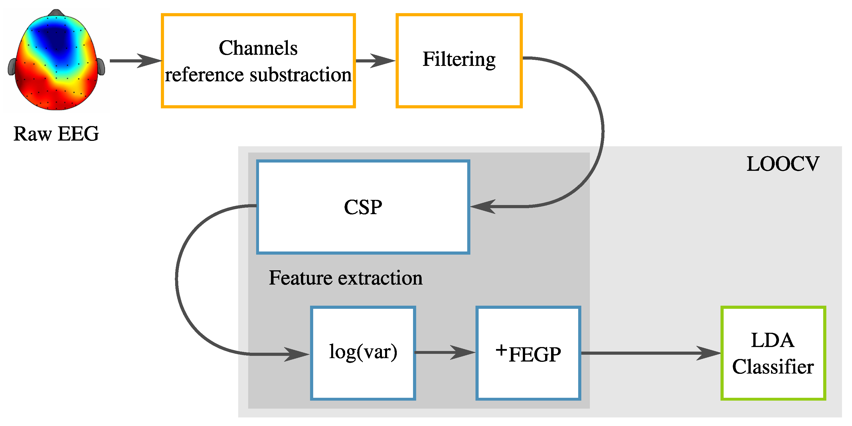
2.2. Pre-Processing
2.3. Common Spatial Patterns
2.4. Classification
3. Proposed Enhanced System
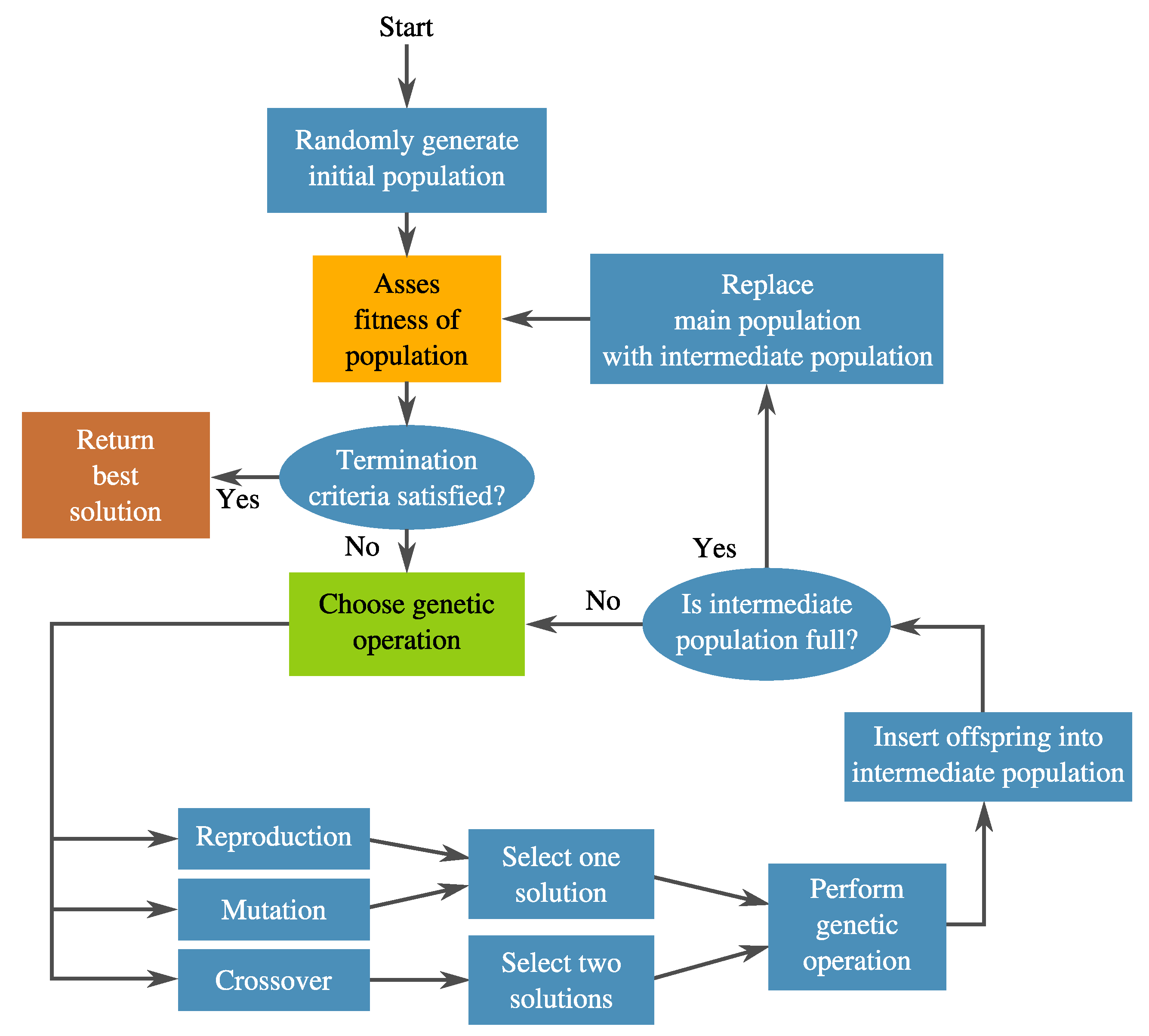
3.1. Genetic Programming
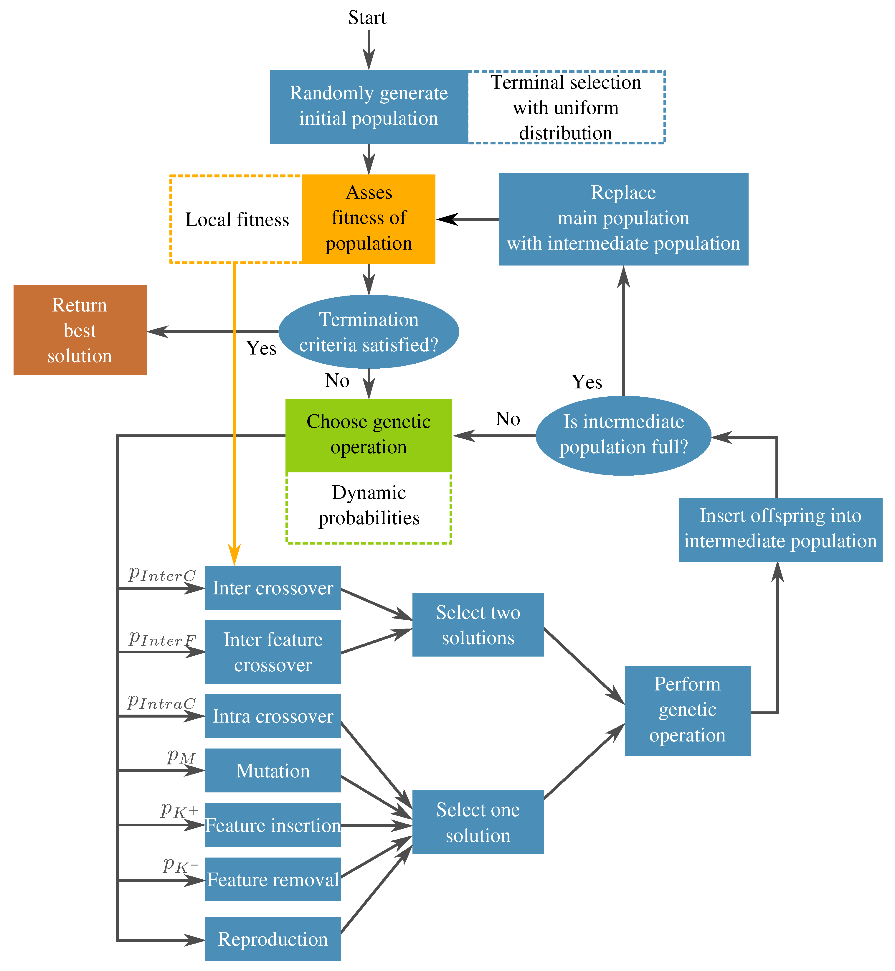
3.2. Augmented Feature Extraction with Genetic Programming: FEGP
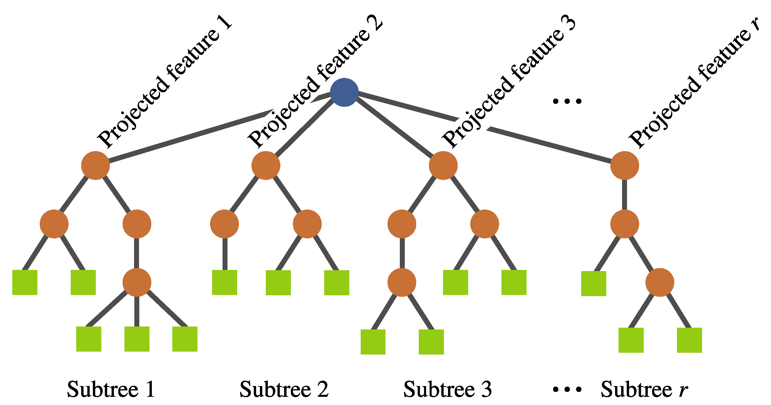
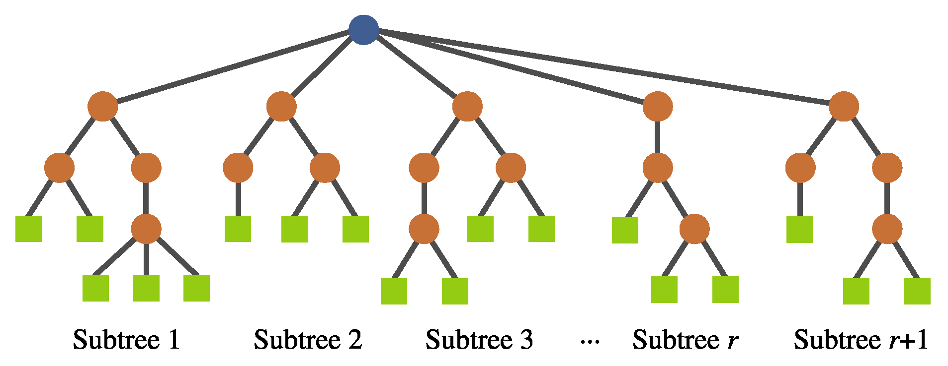
- Individual representation. The representation is also based on a tree structure, but it involves a multi-tree with a single root node, such that each individual defines a mapping of the form , where k is the number of input features and r is the number of newly constructed features. Each of these subtrees are constructed in the same way as in a canonical GP (see Figure 7). No calculation is executed at the root node; it is rather used as a container for the output of the evolving r subtrees. Each subtree works as a non-linear transformation of the input features into a new space that is expected to simplify the classification. Moreover, the number of new features r can vary among individuals.
- New genetic operators. Because of the manner in which individuals are represented, it is necessary to introduce new search operators. For any of these operators, the root node is avoided during the operation to preserve the representation.
- (a)
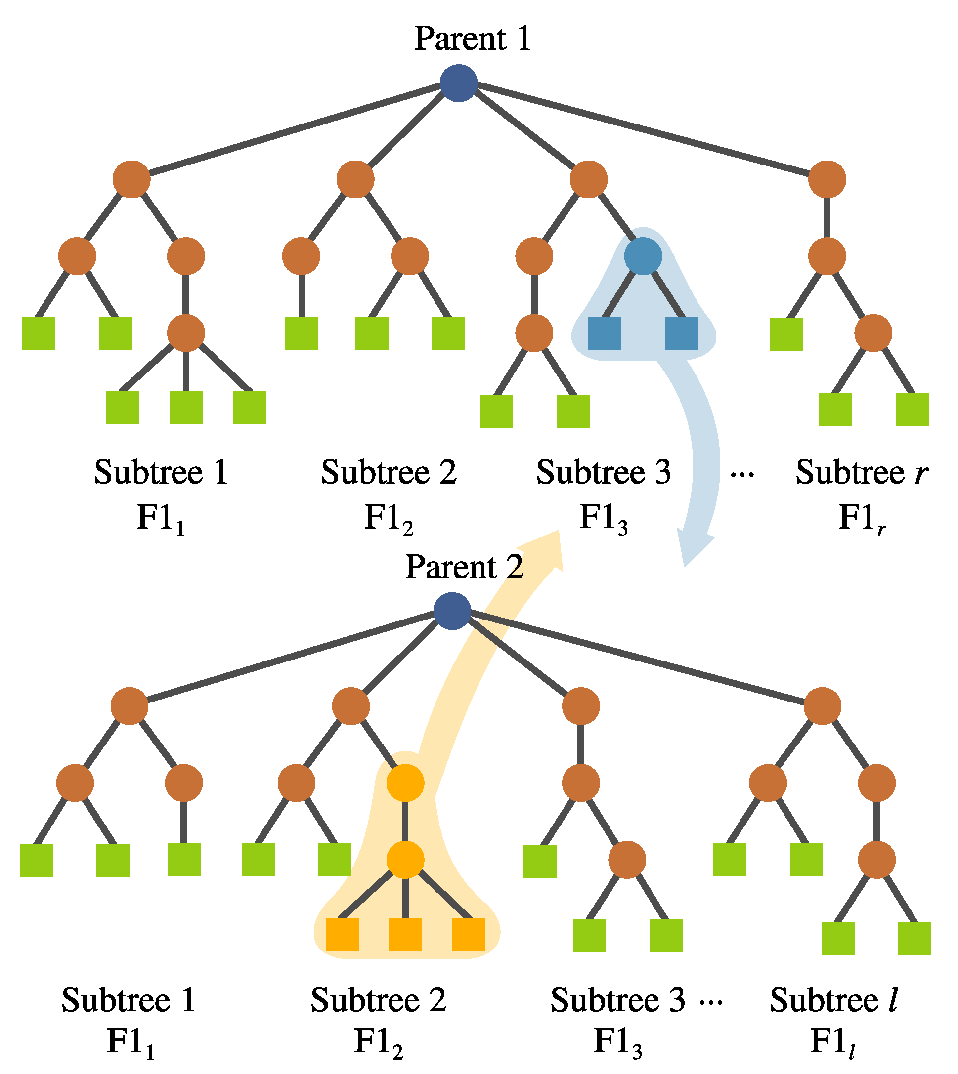
- Inter-crossover. This is a crossover performed between subtrees belonging to different individuals, which produces two offspring. The selection for the crossover points is based on a local fitness measure (discussed in detail later), which allows the best subtrees to interchange genetic material. This is visualized in Figure 8.
- (b)
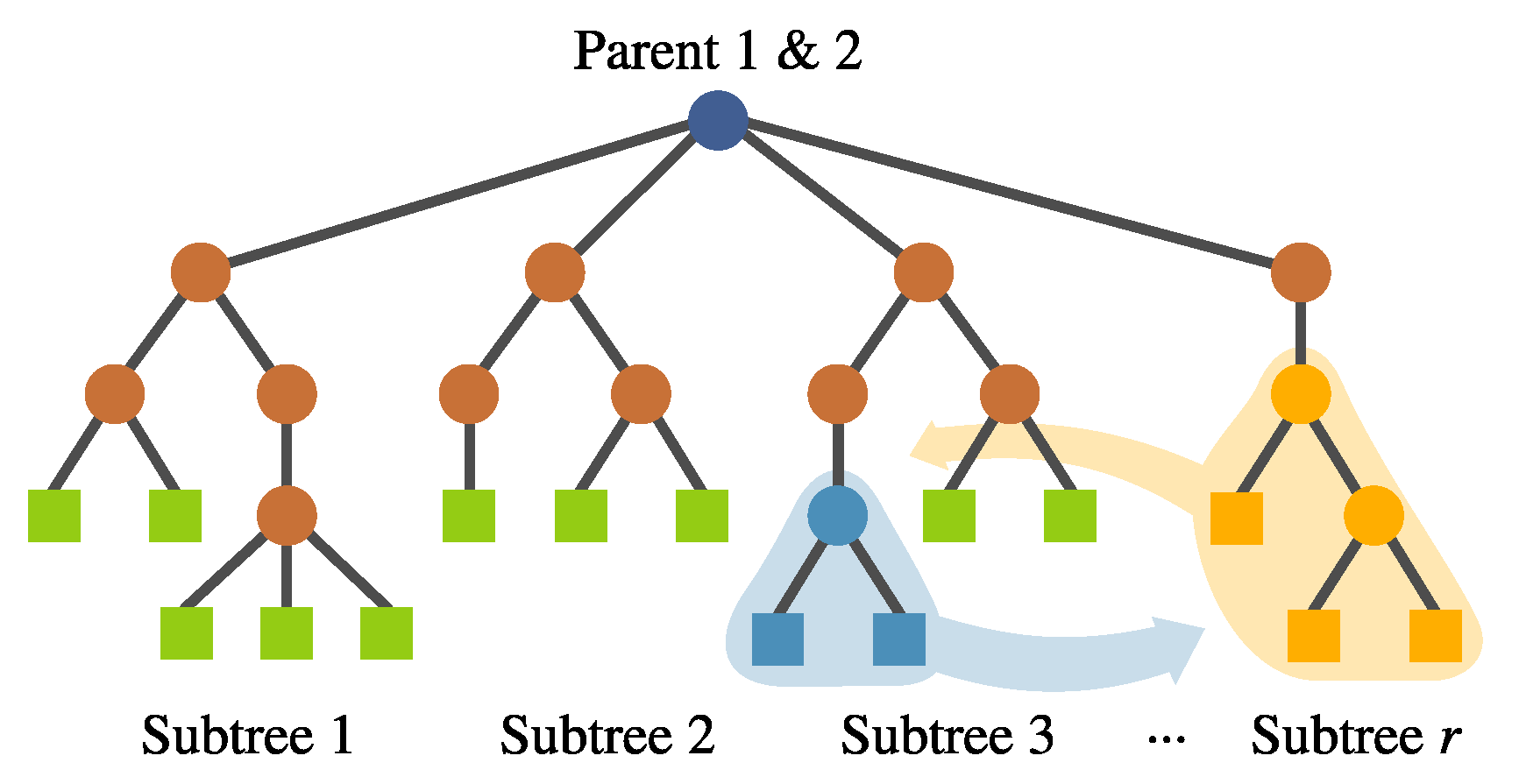
- Intra-crossover. For a given individual, genetic material can be swapped within the same individual using this operator, depicted in Figure 9. The rationale behind this is that genetic material from one feature might help the evolution of another within the same individual, improving the overall fitness. The subtree selection is performed randomly, choosing the crossover points from different subtrees. This operator generates two offspring.
- (c)
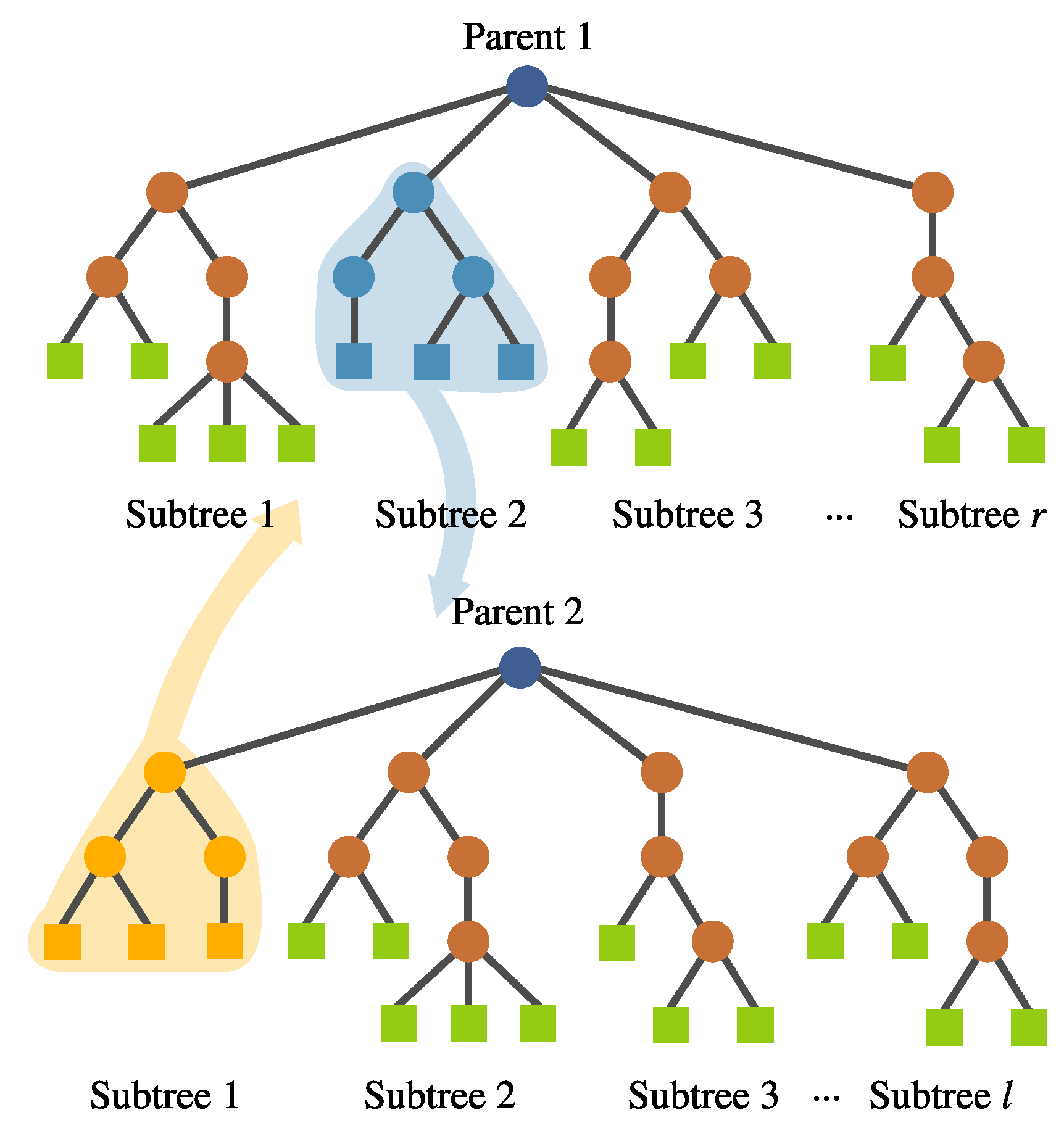
- Inter-individual feature crossover. It can be desirable to keep complete features with good performance within the population. This operator interchanges complete subtrees between two selected individuals. This is performed randomly rather than using a deterministic approach. Preliminary experimentation suggested that avoiding a fitness-based selection of the subtree allowed the algorithm to explore the solution space better. This operator can be seen in Figure 10.
- (d)
- Subtree mutation. This is performed the same way as in canonical GP. A portion of a selected subtree is substituted with a randomly generated tree.
- (e)
- Feature insertion mutation. This operator allows the insertion of a new randomly generated subtree, expanding the dimensionality of the transformed feature space; Figure 11 depicts this operator.
- (f)
- Feature removal mutation. Similarly, a deletion operator is needed to reduce the new feature space. The subtree to be removed is selected randomly. This operator can only be used if .
- Terminal selection during population initialization. In a canonical GP, the initial trees are built by randomly choosing a function or terminal from the available sets in an iterative fashion. This selection process is commonly referred to as sampling with replacement, which could lead to some variables not being chosen as terminal elements in the initial population; the probability of this happening will increase when the number of input features is large. If this is the case, then the initial generations will lack proper exploration of the search space, particularly in the terminal elements, which may lead the search toward local optima. A simple mechanism to avoid this is to enforce that every variable is chosen at least one time as a terminal element in a GP individual. This can be achieved by performing a sampling without replacement of the input features in the terminal set of the GP search. When a terminal is randomly selected, then it is excluded on the subsequent terminal selection steps until all available terminals have been chosen; then, the procedure is repeated by making all terminals available to the tree generation algorithm, such as full, grow, or Ramped Half and Half.
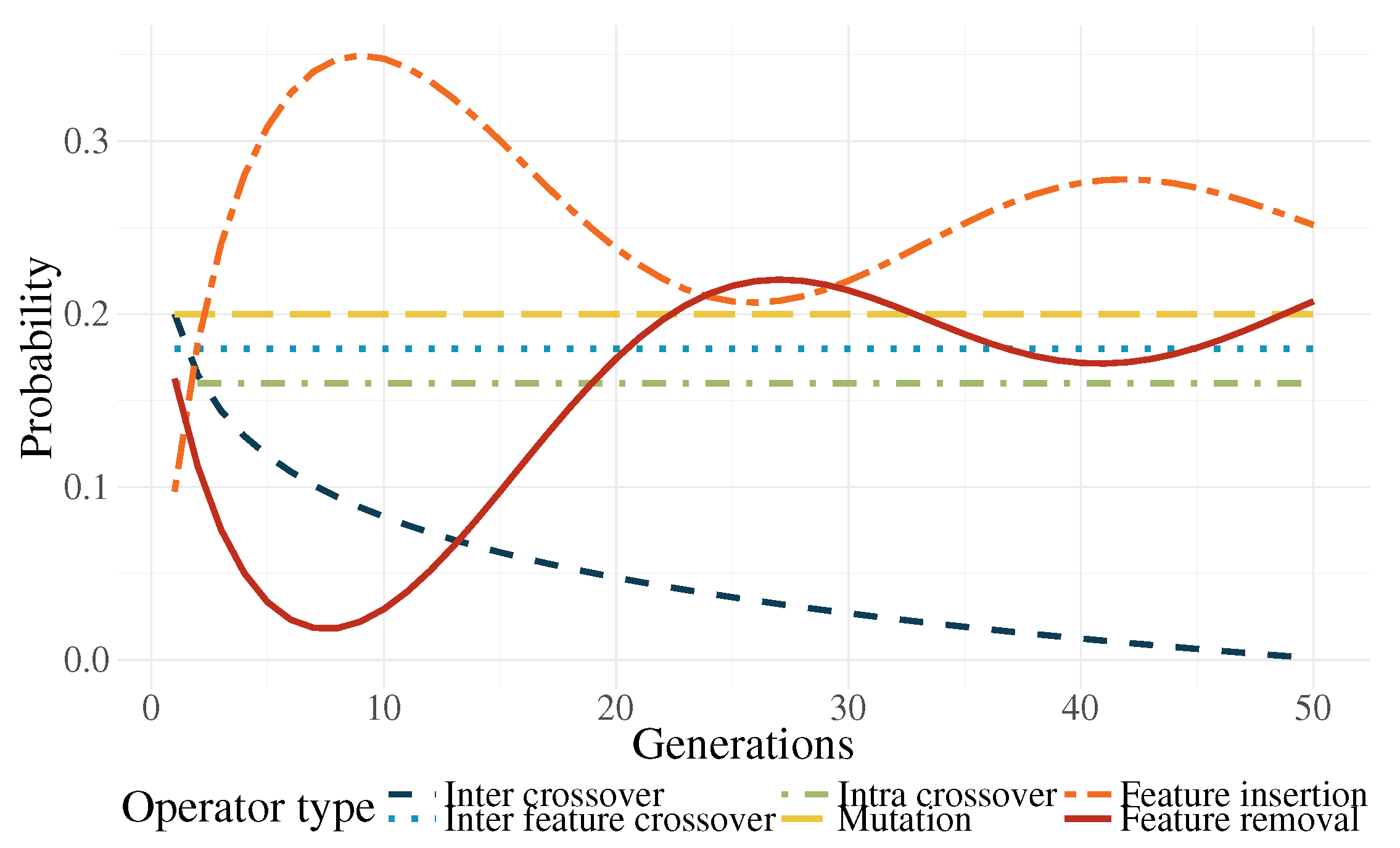
- Genetic operator selection. In canonical GP, operators are chosen at each generation with a user-defined probability. The probability of choosing each operator is usually static throughout the search. In the work by Tuson and Ross [60], their operator probabilities are changed at each generation by rewarding or penalizing operators according with their success at producing good offspring (offspring with high fitness). After an initial preliminary experimentation, we propose functions that modify the operator probabilities based on the work of Tuson and Ross.Based on [60], three operator probabilities (intra-crossover: , inter-individual feature crossover: , and subtree mutation: ) are given by a common dynamic behavior, with the following characteristics: They are periodic, the variation range is rather small, and they are stationary. For simplicity, this condition was replaced by a constant value; in early experimentation, the system behaved almost identically to the algorithm by [60].The other three operators (inter-crossover: , feature insertion mutation: , and feature removal mutation: ) exhibited unique dynamic behaviors using the algorithm by [60]. Here, we proposed the following equations to mimic the behavior of the aforementioned algorithm:where is the current generation, is the maximum generation number, is a decay parameter, and is an initial probability. In preliminary tests, it was found out that, only in the earlier generations, a high probability for the inter-crossover operator was required, mainly to promote the exchange of genetic material and allow the algorithm to do a more efficient search. In more advanced stages of the evolutionary process, this operator produced a negative effect in the search by curtailing the ability of the algorithm to perform exploration. As a countermeasure to this phenomenon, the selection probability for this operator is reduced.Two of the most important operators are the feature insertion and removal mutations. Indeed, these are the ones responsible for the flexibility of the new feature space size. There is a higher probability that the hyperplane of the classifier has a good class separability when the number of dimensions is high. A high probability for the generation of new features () at the start of the run promotes the search for the most promising size of the new feature space. The ratio between these operators and the static ones decreases after the initial generations, giving more importance to the evolution of the solutions without changing the feature space too much. Because evolved models stagnate at the end of the run, increasing the feature space size is required once more. Moreover, (features removal) is seen as the complementary part of and . The operator functions are plotted in Figure 12 for the case that .
- Fitness calculation. The fitness is computed by a local and a global measure, which are used differently by the search. More specifically:
- (a)
- Local fitness measure (Fisher’s Discriminant Ratio). This is computed at the subtree level, which provides a separability value for each constructed feature. Certainly, the quality of a solution depends on the quality of their individual features. The local measure is only used as the criterion for the inter-crossover subtree selection, that is, crossover points are selected within the subtrees with the best local fitness. Although the GP selection process chooses two individuals with similar fitness rank, it does not guarantee that all individual subtrees have a good performance. The goal is for the crossover to exchange features that show good performance in terms of class separation. This is given bywhere , , , and are the means and standard deviations corresponding to class one and two for the ith feature [61]. For any given tree K, r local fitness measures are calculated. It was found that the use of the local fitness in other operators did not help the search.
- (b)
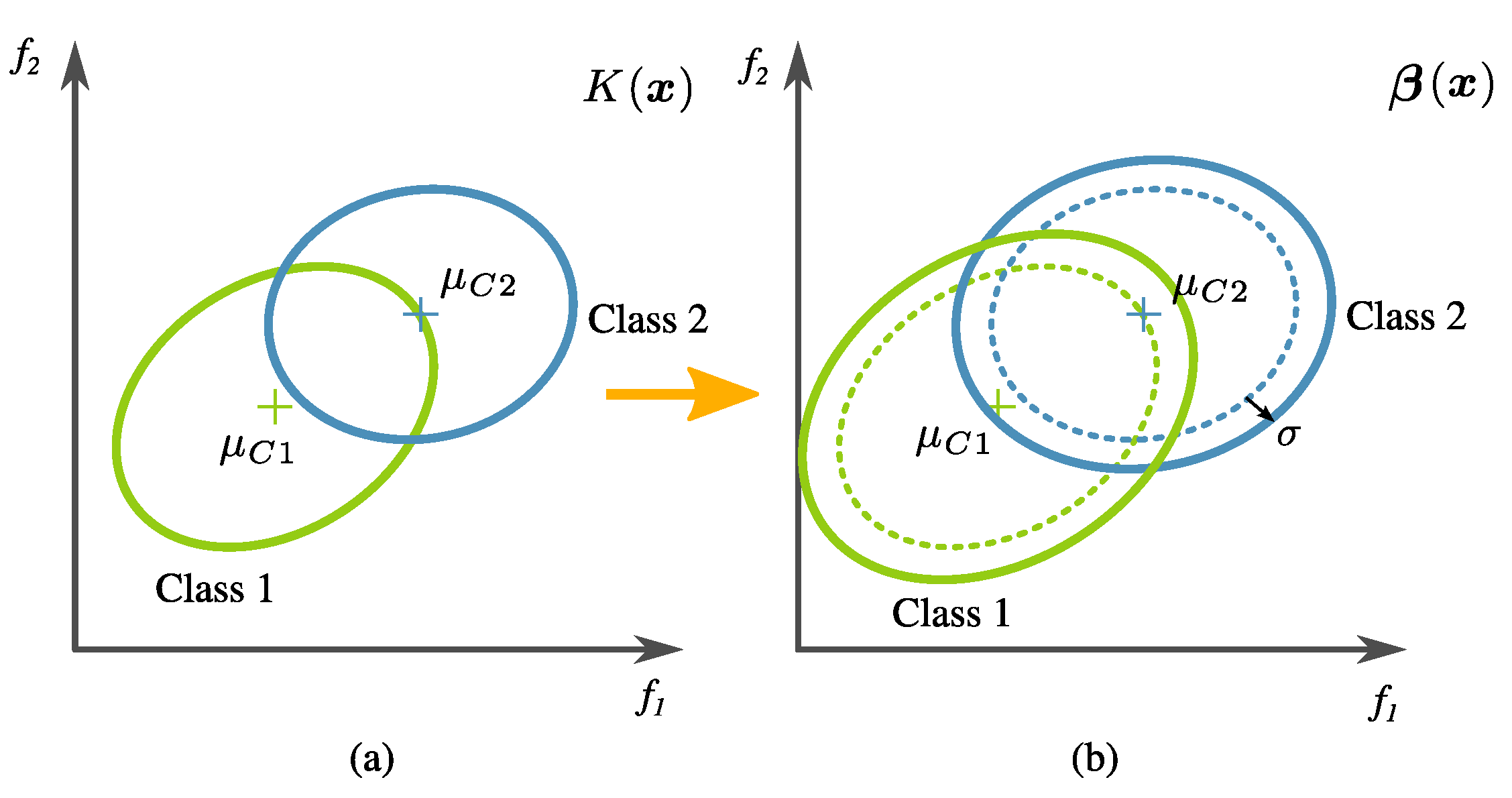
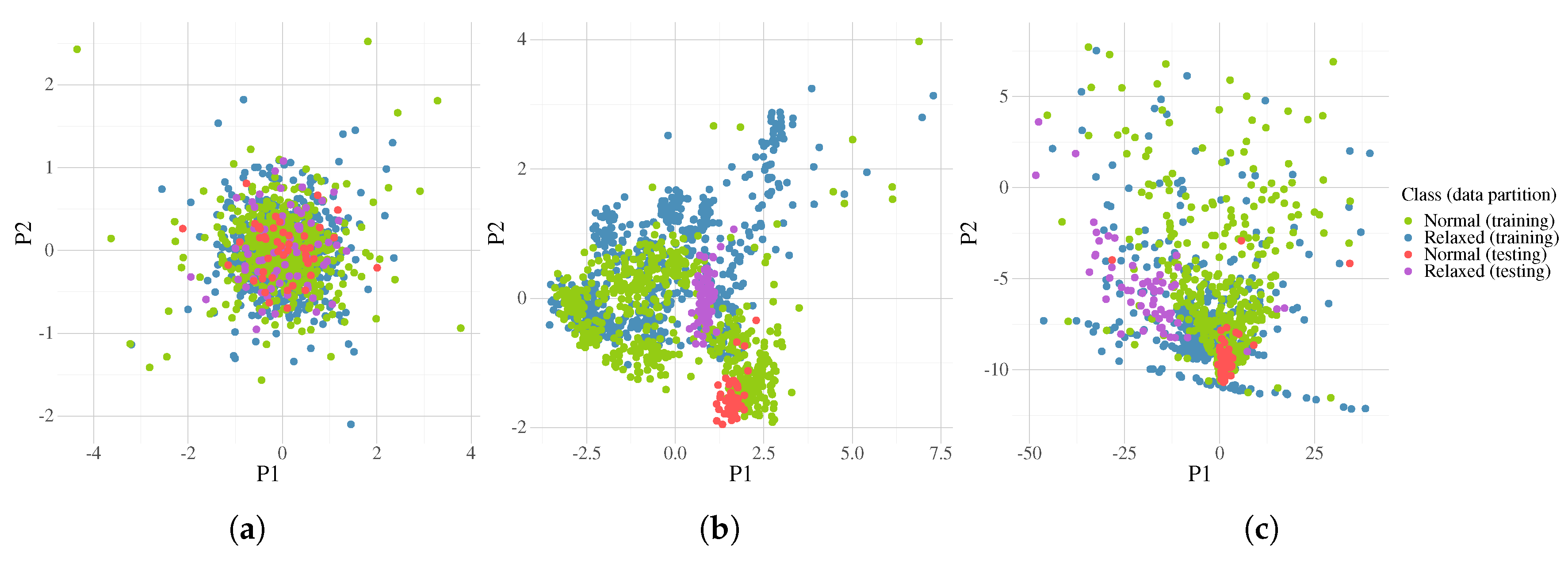
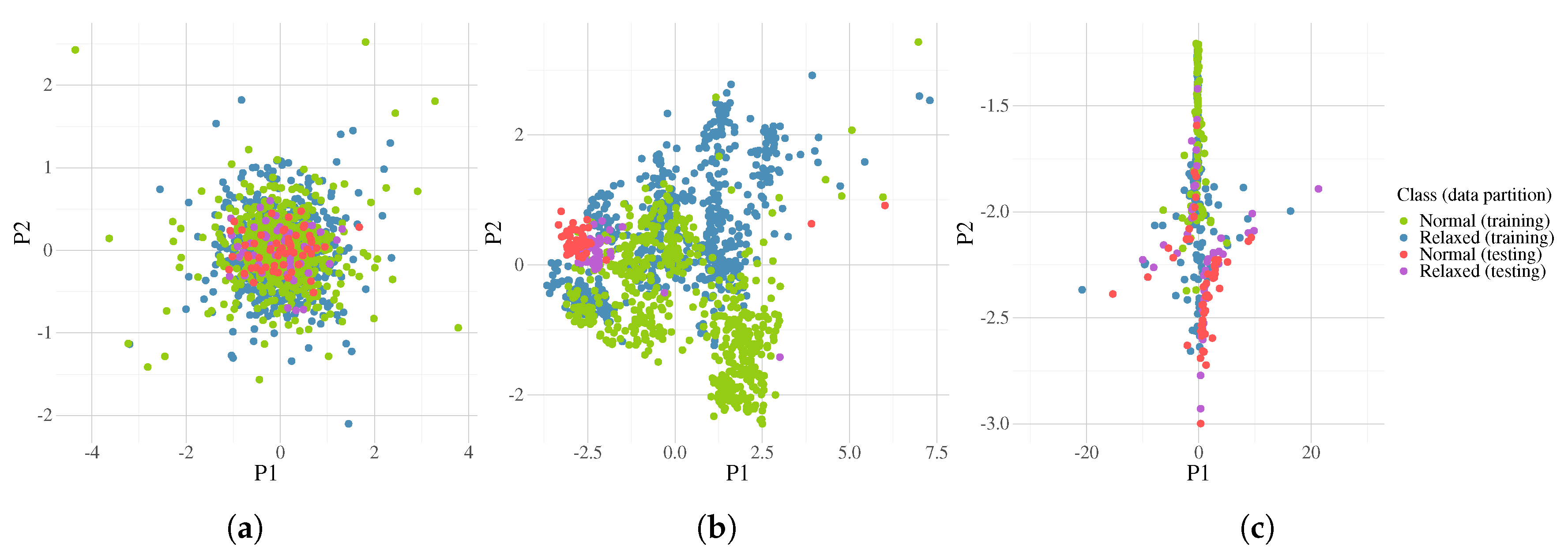
- Global fitness measure. The calculation of global fitness is the result of a two-tier process.In the first level, an initial regularization is performed over the tree output using the training data; then, the classification accuracy () is calculated. In detail, this is done by artificially changing the covariance of transformed training data (i.e., the training data in the new feature space created by an evolved transformation), defined byandwhere denotes the tree output corresponding to all the data samples from class (normal), and is the same but corresponding to class (relaxed). The main reason for this is that data variance is high in this problem, and the classifier training has to be relaxed so that prediction accuracy on unseen data increases. Please note that the actual penalty is given by a factor of twice the standard deviation of the transformed training data. This is exemplified in Figure 13. The confusion matrix is calculated using LDA over the modified data. The classification accuracy is specifically computed withwhere TP (True Positive), TN (True Negative), FN (False Negative), and FP (False Positive) are values from the confusion matrix as a result of the labels .In the second level of the two-tier process, the global fitness is computed bywhere is a proposed second regularization term, given bywhich becomes zero if FP and FN are equal. In preliminary experimentation, it was found that the algorithm tended to avoid over-fitting when there was a balance in the FN and FP scores.
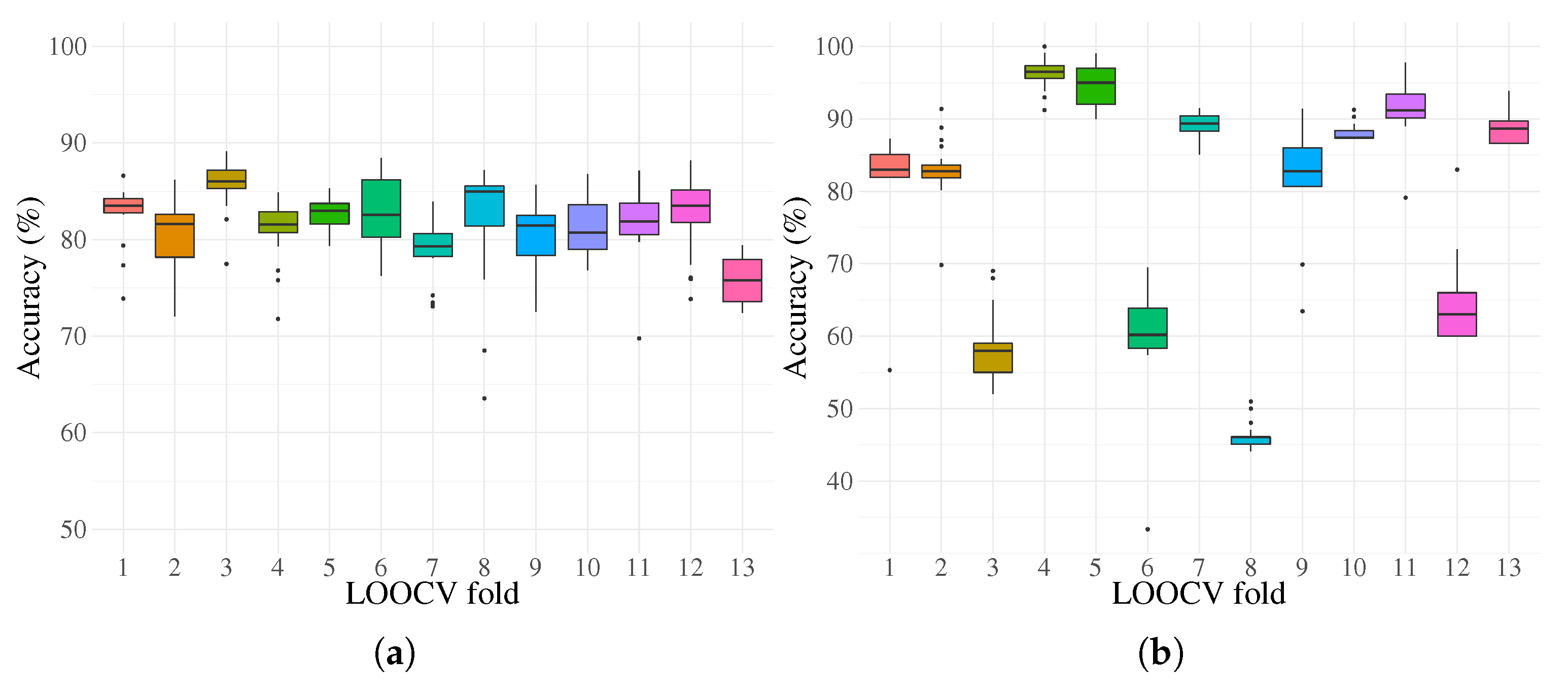
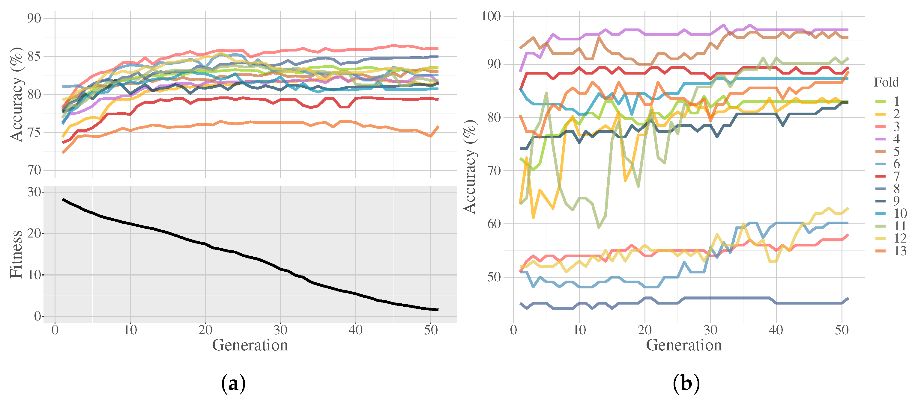
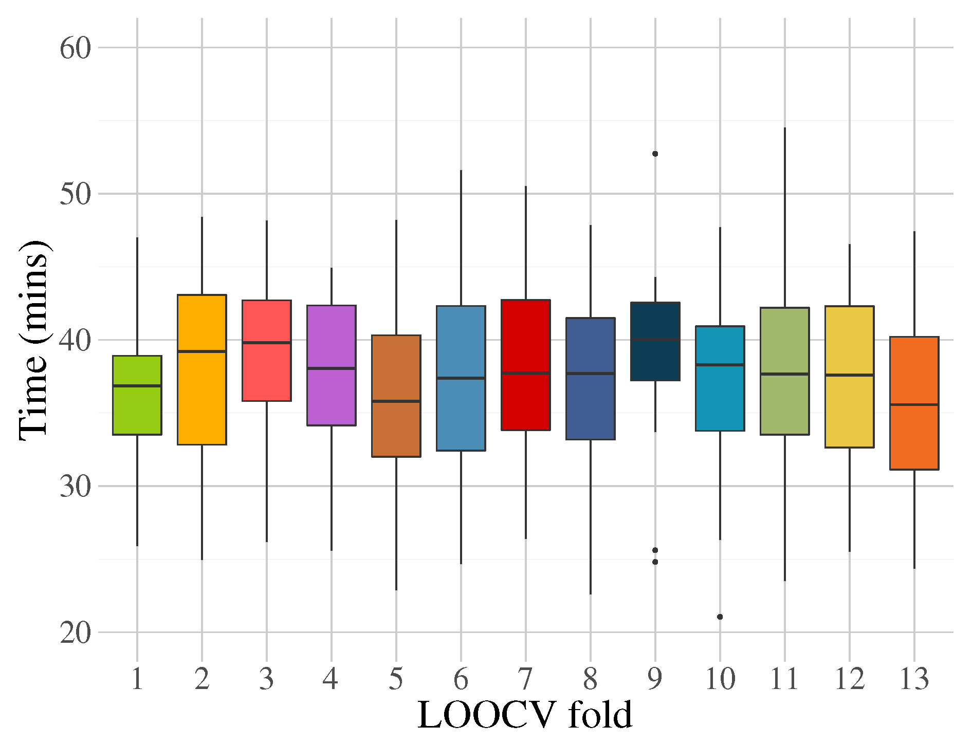
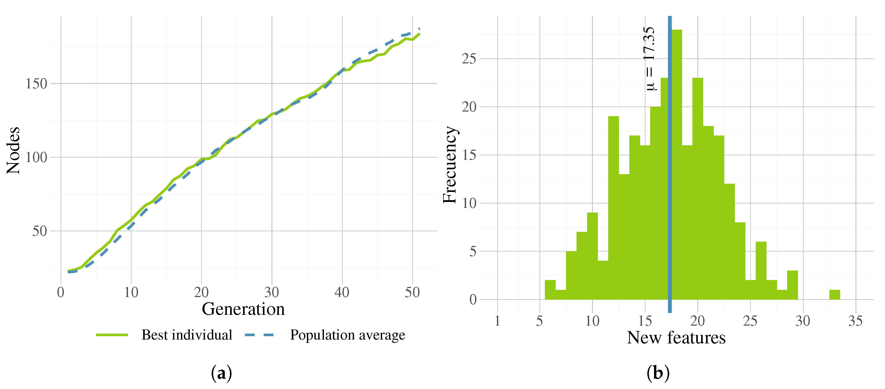
4. Experimentation and Results
5. Discussion
6. Conclusions and Future Work
Author Contributions
Funding
Conflicts of Interest
References
- Alhola, P.; Plo-Kantola, P. Sleep deprivation: Impact on cognitive performance. Neuropsychiatr. Dis. Treat. 2007, 3, 553–567. [Google Scholar]
- Schmidt, E.; Kincses, W.; Schrauf, M. Assessing driver’s vigilance state during monotonous driving. In Proceedings of the Fourth International Driving Symposium on Human Factors in Driver Assessment, Training and Vehicle Design, Stevenson, Washington, DC, USA, 10 October 2007; pp. 138–145. [Google Scholar]
- Selye, H. The Stress Syndrome. Am. J. Nurs. 1965, 65, 97–99. [Google Scholar]
- Baars, B. A Cognitive Theory of Consciousness; Cambridge University Press: Cambridge, UK, 1988. [Google Scholar]
- Laureys, S. The neural correlate of (un)awareness: Lessons from the vegetative state. Trends Cogn. Sci. 2005, 9, 556–559. [Google Scholar] [CrossRef] [PubMed]
- Prashant, P.; Joshi, A.; Gandhi, V. Brain computer interface: A review. In Proceedings of the 2015 5th Nirma University International Conference on Engineering (NUiCONE), Ahmedabad, India, 25 May 2015; Volume 74, pp. 1–6. [Google Scholar]
- Myrden, A.; Chau, T. Effects of user mental state on EEG-BCI performance. Front. Hum. Neurosci. 2015, 9, 308. [Google Scholar] [CrossRef] [PubMed]
- Siuly, S.; Li, Y.; Zhang, Y. EEG Signal Analysis and Classification: Techniques and Applications; Health Information Science, Springer International Publishing: Cham, Switzerland, 2017. [Google Scholar]
- Vézard, L.; Legrand, P.; Chavent, M.; Faïta-Aïnseba, F.; Trujillo, L. EEG classification for the detection of mental states. Appl. Soft Comput. 2015, 32, 113–131. [Google Scholar] [CrossRef]
- Muñoz, L.; Silva, S.; Trujillo, L. M3GP—Multiclass Classification with GP. In Genetic Programming, Proceedings of the 18th European Conference, EuroGP 2015, Copenhagen, Denmark, 8–10 April 2015; Springer International Publishing: Cham, Switzerland, 2015; pp. 78–91. [Google Scholar]
- Woodman, G.F. A brief introduction to the use of event-related potentials (ERPs) in studies of perception and attention. Atten. Percept. Psychophysiol. 2010, 72, 1–29. [Google Scholar]
- Nicolas-Alonso, L.F.; Gomez-Gil, J. Brain computer interfaces, a review. Sensors 2012, 12, 1211–1279. [Google Scholar] [CrossRef]
- Amiri, S.; Fazel-rezai, R.; Asadpour, V. A Review of Hybrid Brain-Computer Interface Systems. Adv. -Hum.-Comput. Interact. - Spec. Issue Using Brain Waves Control. Comput. Mach. 2013, 1–8. [Google Scholar] [CrossRef]
- Gupta, A.; Agrawal, R.K.; Kaur, B. Performance enhancement of mental task classification using EEG signal: A study of multivariate feature selection methods. Soft Comput. 2015, 19, 2799–2812. [Google Scholar] [CrossRef]
- Trejo, L.J.; Kubitz, K.; Rosipal, R.; Kochavi, R.L.; Montgomery, L.D. EEG-Based Estimation and Classification of Mental Fatigue. Psychology 2015, 6, 572–589. [Google Scholar] [CrossRef]
- Zarjam, P.; Epps, J.; Lovell, N.H. Beyond Subjective Self-Rating: EEG Signal Classification of Cognitive Workload. IEEE Trans. Auton. Ment. Dev. 2015, 7, 301–310. [Google Scholar] [CrossRef]
- Garcés Correa, A.; Orosco, L.; Laciar, E. Automatic detection of drowsiness in EEG records based on multimodal analysis. Med. Eng. Phys. 2014, 36, 244–249. [Google Scholar] [CrossRef] [PubMed]
- Hariharan, M.; Vijean, V.; Sindhu, R.; Divakar, P.; Saidatul, A.; Yaacob, S. Classification of mental tasks using stockwell transform. Comput. Electr. Eng. 2014, 40, 1741–1749. [Google Scholar] [CrossRef]
- Mallikarjun, H.M.; Suresh, H.N.; Manimegalai, P. Mental State Recognition by using Brain Waves. Indian J. Sci. Technol. 2016, 9, 2–6. [Google Scholar] [CrossRef]
- Schultze-Kraft, M.; Dähne, S.; Gugler, M.; Curio, G.; Blankertz, B. Unsupervised classification of operator workload from brain signals. J. Neural Eng. 2016, 13, 036008. [Google Scholar] [CrossRef]
- Wu, W.; Chen, Z.; Gao, X.; Li, Y.; Brown, E.N.; Gao, S. Probabilistic common spatial patterns for multichannel EEG analysis. IEEE Trans. Pattern Anal. Mach. Intell. 2015, 37, 639–653. [Google Scholar] [CrossRef]
- Arvaneh, M.; Guan, C.; Ang, K.K.; Ward, T.E.; Chua, K.S.; Kuah, C.W.K.; Ephraim Joseph, G.J.; Phua, K.S.; Wang, C. Facilitating motor imagery-based brain–computer interface for stroke patients using passive movement. Neural Comput. Appl. 2017, 28, 3259–3272. [Google Scholar] [CrossRef]
- Hajinoroozi, M.; Mao, Z.; Huang, Y. Prediction of driver’s drowsy and alert states from EEG signals with deep learning. In Proceedings of the 2015 IEEE 6th International Workshop on Computational Advances in Multi-Sensor Adaptive Processing, CAMSAP 2015, Cancun, Mexico, 13–16 December 2015; pp. 493–496. [Google Scholar]
- Saidatul, A.; Paulraj, S.Y. Mental Stress Level Classification Using Eigenvector Features and Principal Component Analysis. Commun. Inf. Sci. Manag. Eng. 2013, 3, 254–261. [Google Scholar]
- Guo, L.; Rivero, D.; Dorado, J.; Munteanu, C.R.; Pazos, A. Automatic feature extraction using genetic programming: An application to epileptic EEG classification. Expert Syst. Appl. 2011, 38, 10425–10436. [Google Scholar] [CrossRef]
- Berek, P.; Prilepok, M.; Platos, J.; Snasel, V. Classification of EEG Signals Using Vector Quantization. In International Conference on Artificial Intelligence and Soft Computing; Springer: Zakopane, Poland, 2014; pp. 107–118. [Google Scholar]
- Shen, K.Q.; Li, X.P.; Ong, C.J.; Shao, S.Y.; Wilder-Smith, E.P.V. EEG-based mental fatigue measurement using multi-class support vector machines with confidence estimate. Clin. Neurophysiol. 2008, 119, 1524–1533. [Google Scholar] [CrossRef]
- Khasnobish, A.; Konar, A.; Tibarewala, D.N. Object Shape Recognition from EEG Signals during Tactile and Visual Exploration. In International Conference on Pattern Recognition and Machine Intelligence; Springer: Kolkata, India, 2013; pp. 459–464. [Google Scholar]
- Vézard, L.; Chavent, M.; Legrand, P.; Faïta-Aïnseba, F.; Trujillo, L. Detecting mental states of alertness with genetic algorithm variable selection. In Proceedings of the 2013 IEEE Congress on Evolutionary Computation, CEC 2013, Cancun, Mexico, 20–23 June 2013; pp. 1247–1254. [Google Scholar]
- Fang, C.; Li, H.; Ma, L. EEG Signal Classification Using the Event-Related Coherence and Genetic Algorithm. In Advances in Brain Inspired Cognitive Systems; Springer: Beijing, China, 2013; pp. 92–100. [Google Scholar]
- Rezaee, A. Applying Genetic Algorithm to EEG Signals for Feature Reduction in Mental Task Classification. Int. J. Smart Electr. Eng. 2016, 5, 4–7. [Google Scholar]
- Hongxia, L.; Hongxi, D.; Jian, L.; Shuicheng, T. Research on the application of the improved genetic algorithm in the electroencephalogram-based mental workload evaluation for miners. J. Algorithms Comput. Technol. 2016, 10, 1–10. [Google Scholar] [CrossRef]
- Orriols-Puig, A.; Casillas, J.; Bernadó-Mansilla, E. A Comparative Study of Several Genetic-Based Supervised Learning Systems. In Learning Classifier Systems in Data Mining; Springer: Berlin, Heidelberg, 2008; Volume 125, pp. 205–230. [Google Scholar]
- Erguzel, T.T.; Ozekes, S.; Gultekin, S.; Tarhan, N. Ant colony optimization based feature selection method for QEEG data classification. Psychiatry Investig. 2014, 11, 243–250. [Google Scholar] [CrossRef] [PubMed]
- Mirvaziri, H.; Mobarakeh, Z.S. Improvement of EEG-based motor imagery classification using ring topology-based particle swarm optimization. Biomed. Signal Process. Control. 2017, 32, 69–75. [Google Scholar] [CrossRef]
- Hassani, K.; Lee, W.s. An Incremental Framework for Classification of EEG Signals Using Quantum Particle Swarm Optimization. In IEEE International Conference on Computational Intelligence and Virtual Environments for Measurement Systems and Applications (CIVEMSA); IEEE: Ottawa, ON, Canada, 2014; pp. 40–45. [Google Scholar]
- Bhardwaj, A.; Tiwari, A.; Varma, M.V.; Krishna, M.R. Classification of EEG signals using a novel genetic programming approach. In Proceedings of the 2014 Conference Companion on Genetic and Evolutionary Computation Companion—GECCO Comp ’14, Vancouver, BC, Canada, 12–16 July 2014; pp. 1297–1304. [Google Scholar]
- Bhardwaj, A.; Tiwari, A.; Krishna, R.; Varma, V. A novel genetic programming approach for epileptic seizure detection. Comput. Methods Programs Biomed. 2016, 124, 2–18. [Google Scholar] [CrossRef]
- Fernández-Blanco, E.; Rivero, D.; Gestal, M.; Dorado, J. Classification of signals by means of Genetic Programming. Soft Comput. 2013, 17, 1929–1937. [Google Scholar] [CrossRef]
- Sotelo, A.; Guijarro, E.; Trujillo, L.; Coria, L.N.; Martínez, Y. Identification of epilepsy stages from {ECoG} using genetic programming classifiers. Comput. Biol. Med. 2013, 43, 1713–1723. [Google Scholar] [CrossRef]
- Lin, J.Y.; Ke, H.R.; Chien, B.C.; Yang, W.P. Designing a classifier by a layered multi-population genetic programming approach. Pattern Recognit. 2007, 40, 2211–2225. [Google Scholar] [CrossRef]
- Chien, B.C.; Lin, J.Y.; Yang, W.P. Learning effective classifiers with -value measure based on genetic programming. Pattern Recognit. 2004, 37, 1957–1972. [Google Scholar] [CrossRef]
- Smart, O.; Firpi, H.; Vachtsevanos, G. Genetic programming of conventional features to detect seizure precursors. Eng. Appl. Artif. Intell. 2007, 20, 1070–1085. [Google Scholar] [CrossRef]
- Sabeti, M.; Katebi, S.; Boostani, R. Entropy and complexity measures for EEG signal classification of schizophrenic and control participants. Artif. Intell. Med. 2009, 47, 263–274. [Google Scholar] [CrossRef] [PubMed]
- Guo, H.; Zhang, Q.; Nandi, A.K. Feature extraction and dimensionality reduction by genetic programming based on the Fisher criterion. Expert Syst. 2008, 25, 444–459. [Google Scholar] [CrossRef]
- Walter, W.G.; Cooper, R.; Aldridge, V.J.; McCallum, W.C.; Winter, A.L. Contingent Negative Variation: An Electric Sign of Sensori-Motor Association and Expectancy in the Human Brain. Nature 1964, 203, 380–384. [Google Scholar] [CrossRef] [PubMed]
- Pfurtscheller, G.; Neuper, C.; Flotzinger, D.; Pregenzer, M. EEG-based discrimination between imagination of right and left hand movement. Electroencephalogr. Clin. Neurophysiol. 1997, 103, 642–651. [Google Scholar] [CrossRef]
- Ramoser, H.; Müller-Gerking, J.; Pfurtscheller, G. Optimal spatial filtering of single trial EEG during imagined hand movement. IEEE Trans. Rehabil. Eng. 2000, 8, 441–446. [Google Scholar] [CrossRef] [PubMed]
- Blankertz, B.; Tomioka, R.; Lemm, S.; Kawanabe, M.; Muller, K.r. Optimizing Spatial filters for Robust EEG Single-Trial Analysis. IEEE Signal Process. Mag. 2008, 25, 41–56. [Google Scholar] [CrossRef]
- Duda, R.O.; Hart, P.E.; Stork, D.G. Pattern Classification, 2nd ed.; Wiley-Interscience: New York, NY, USA, 2000. [Google Scholar]
- Koza, J.R. Genetic Programming: On the Programming of Computers by Means of Natural Selection; MIT Press: Cambridge, MA, USA, 1992. [Google Scholar]
- Goldberg, D.E. Genetic Algorithms in Search, Optimization and Machine Learning, 1st ed.; Addison-Wesley Longman Publishing Co., Inc.: Boston, MA, USA, 1989. [Google Scholar]
- Koza, J.R. Human-competitive results produced by genetic programming. Genet. Program. Evolvable Mach. 2010, 11, 251–284. [Google Scholar] [CrossRef]
- O’Neill, M.; Vanneschi, L.; Gustafson, S.; Banzhaf, W. Open issues in Genetic Programming. Genet. Program. Evolvable Mach. 2010, 11, 339–363. [Google Scholar] [CrossRef]
- Hastie, T.; Tibshirani, R.; Friedman, J.; Hastie, T.; Friedman, J.; Tibshirani, R. The Elements of Statistical Learning: Data Mining, Inference, and Prediction; Springer: Berlin/Heidelberg, Germany, 2009; Volume 2. [Google Scholar]
- Cawley, G.C.; Talbot, N.L.C. On Over-fitting in Model Selection and Subsequent Selection Bias in Performance Evaluation. J. Mach. Learn. Res. 2010, 11, 2079–2107. [Google Scholar]
- Naredo, E.; Trujillo, L.; Legrand, P.; Silva, S.; Muñoz, L. Evolving genetic programming classifiers with novelty search. Inf. Sci. 2016, 369, 347–367. [Google Scholar] [CrossRef]
- Firpi, H.; Goodman, E.; Echauz, J. On prediction of epileptic seizures by means of genetic programming artificial features. Ann. Biomed. Eng. 2006, 34, 515–529. [Google Scholar] [CrossRef] [PubMed]
- Poli, R.; Salvaris, M.; Cinel, C. Evolution of a brain-computer interface mouse via genetic programming. Lect. Notes Comput. Sci. (Including Subser. Lect. Notes Artif. Intell. Lect. Notes Bioinf.) 2011, 6621 LNCS, 203–214. [Google Scholar]
- Tuson, A.; Ross, P. Adapting operator settings in genetic algorithms. Evol. Comput. 1998, 6, 161–184. [Google Scholar] [CrossRef] [PubMed]
- Ho, T.K.; Basu, M. Complexity measures of supervised classification problems. IEEE Trans. Pattern Anal. Mach. Intell. 2002, 24, 289–300. [Google Scholar]
- Silva, S.; Almeida, J. GPLAB—A genetic programming toolbox for MATLAB. In Proceedings of the Nordic MATLAB Conference, Copenhagen, Denmark, 21–22 October 2003; pp. 273–278. [Google Scholar]
- Silva, S.; Costa, E. Dynamic limits for bloat control in genetic programming and a review of past and current bloat theories. Genet. Program. Evolvable Mach. 2009, 10, 141–179. [Google Scholar] [CrossRef]
- Jaiantilal, A. RF Matlab Interface, Version 0.02, Github. Available online: https://github.com/ajaiantilal/randomforest-matlab (accessed on 22 August 2020).
- Z-Flores, E.; Trujillo, L.; Schütze, O.; Legrand, P. Evaluating the Effects of Local Search in Genetic Programming. In EVOLVE—A Bridge between Probability, Set Oriented Numerics, and Evolutionary Computation V; Springer International Publishing: Cham, Switzerland, 2014; Volume 288, pp. 213–228. [Google Scholar]
- Z-Flores, E.; Trujillo, L.; Schütze, O.; Legrand, P. A Local Search Approach to Genetic Programming for Binary Classification. In Proceedings of the 2015 on Genetic and Evolutionary Computation Conference-GECCO ’15, Madrid, Spain, 11–15 July 2015; pp. 1151–1158. [Google Scholar]


| Parameter | Value | Comments |
|---|---|---|
| Generations | 50 | If the max depth for the evolved trees is relatively small, then more generations are not needed, since the solution size is restricted and the overall search stagnates. |
| Population size | 100 | A small population was found to be sufficient to evolve good solutions with larger populations, reaching the same performance. |
| Population initialization | Full | Since the search space can be huge, very small individuals are not beneficial to quickly explore the solution space. |
| Population init max depth | 5 levels | A good compromise between structure diversity and complexity. |
| Initial features | 3 | Variable r. |
| Search operators | Inter-crossover, inter-feature crossover, intra-crossover, mutation, feature insertion, feature removal | |
| Initial probabilities for search operators | 0.2, 0.2, 0.2, 0.05, 0.15, 0.1 | Each value corresponds to each operator in the same order as the above list. |
| Delta values for decay function | 0.2 | This only applies to the inter-crossover operator. |
| Function set | +,−,×,/,log,cos,sin, tan,√,abs | |
| Terminal set | random [0,1], input features | |
| Max depth level | 20 | Since individuals can have several features, big values for the allowed depth are not desired. If a child tree is above this limit after the genetic operation, then it is discarded and a reproduction operation is performed instead. |
| Selection | Tournament, size 5 | A small tournament size provides a richer diversity in the population. |
| Elitism | Only best individual survives | Assures that the best solution is not lost from generation to generation. |
| 1 | 2 | 3 | 4 | 5 | 6 | 7 | 8 | 9 | 10 | 11 | 12 | 13 | ||
|---|---|---|---|---|---|---|---|---|---|---|---|---|---|---|
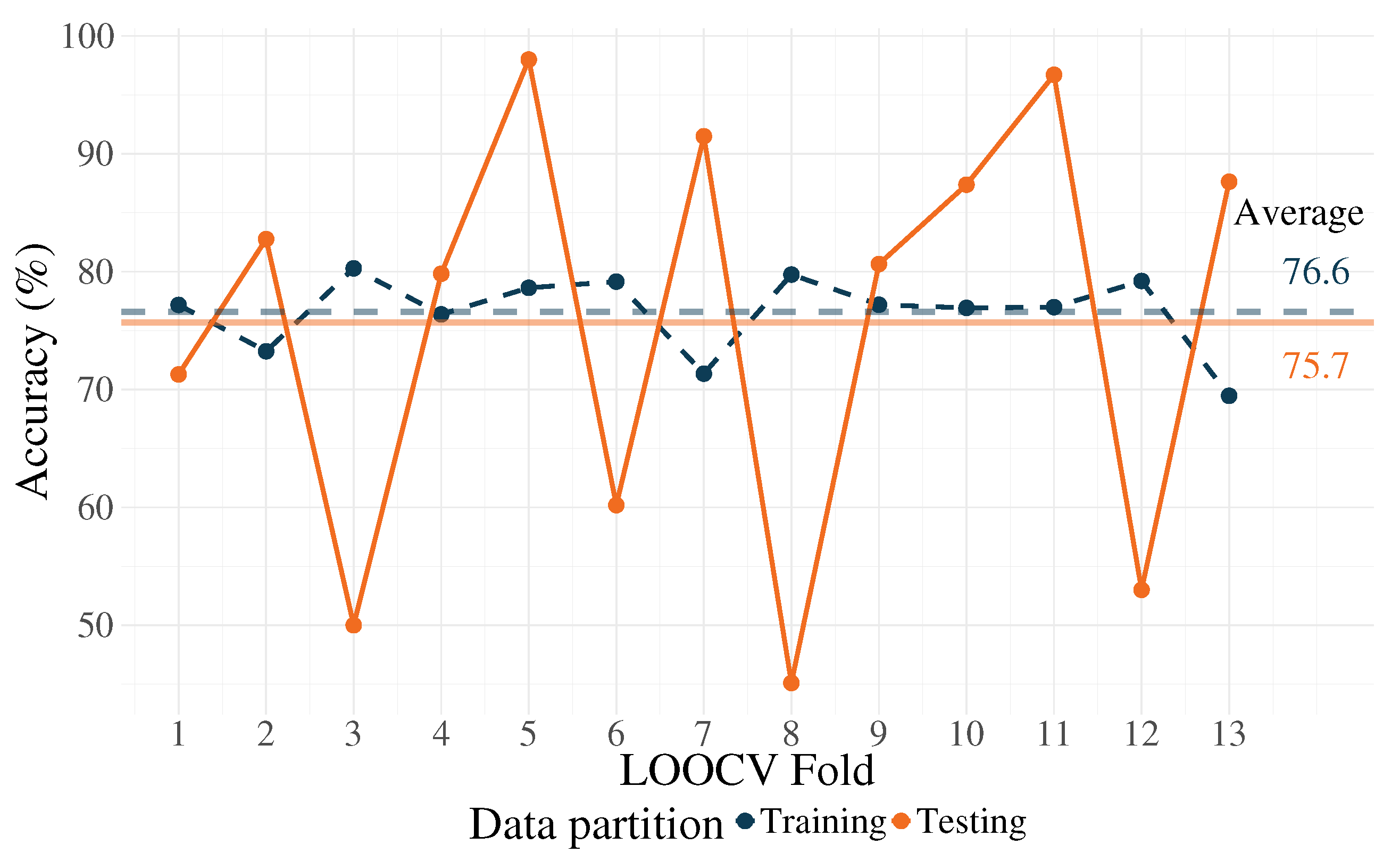
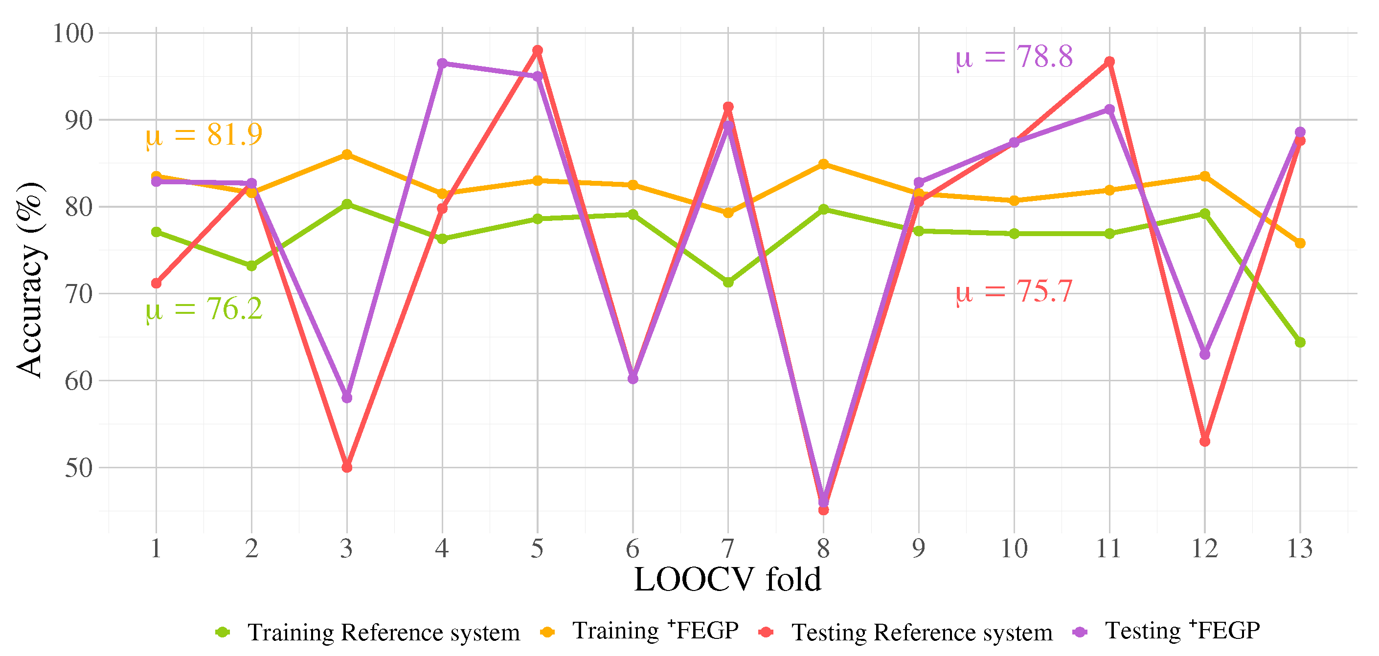
| Training | Accuracy | 83.5 | 81.6 | 86 | 81.5 | 83 | 82.5 | 79.3 | 84.9 | 81.5 | 80.7 | 81.9 | 83.5 | 75.8 |
| 0.70 | 0.68 | 0.77 | 0.63 | 0.72 | 0.56 | 0.72 | 0.77 | 0.64 | 0.49 | 0.77 | 0.69 | 0.63 | ||
| p-value | 0.0000 | 0.0000 | 0.0000 | 0.0000 | 0.0000 | 0.0000 | 0.0000 | 0.0000 | 0.0000 | 0.0000 | 0.0000 | 0.0000 | 0.0000 | |
| Testing | Accuracy | 82.9 | 82.7 | 58 | 96.5 | 95 | 60.2 | 89.3 | 46 | 82.8 | 87.4 | 91.2 | 63 | 88.6 |
| 0.70 | 0.65 | 0.16 | 0.90 | 0.88 | 0.30 | 0.79 | 0.01 | 0.72 | 0.81 | 0.78 | 0.24 | 0.75 | ||
| p-value | 0.0000 | 0.0000 | 0.3346 | 0.0000 | 0.0000 | 0.0023 | 0.0000 | 0.9702 | 0.0000 | 0.0000 | 0.0000 | 0.1379 | 0.0000 |
| 1 | 2 | 3 | 4 | 5 | 6 | 7 | 8 | 9 | 10 | 11 | 12 | 13 | |
|---|---|---|---|---|---|---|---|---|---|---|---|---|---|
| 1 | - | 0.0011 | 0.0000 | 0.0108 | 0.3038 | 0.0706 | 0.0000 | 0.0108 | 0.0003 | 0.0108 | 0.0290 | 0.3038 | 0.0000 |
| 2 | 0.0168 | - | 0.0000 | 0.5309 | 0.0706 | 0.3038 | 0.0706 | 0.0108 | 0.9728 | 0.9728 | 0.1545 | 0.0290 | 0.0001 |
| 3 | 0.0001 | 0.0000 | - | 0.0000 | 0.0000 | 0.0036 | 0.0000 | 0.0108 | 0.0000 | 0.0001 | 0.0003 | 0.0036 | 0.0000 |
| 4 | 0.0206 | 0.6327 | 0.0000 | - | 0.1545 | 0.3038 | 0.0011 | 0.0036 | 0.7974 | 0.5309 | 0.7974 | 0.0290 | 0.0000 |
| 5 | 0.5799 | 0.0442 | 0.0000 | 0.0741 | - | 0.3038 | 0.0001 | 0.0290 | 0.1545 | 0.0290 | 0.5309 | 0.5309 | 0.0000 |
| 6 | 0.6326 | 0.1589 | 0.0103 | 0.2683 | 0.8602 | - | 0.0036 | 0.3038 | 0.3038 | 0.5309 | 0.7974 | 0.5309 | 0.0000 |
| 7 | 0.0001 | 0.1020 | 0.0000 | 0.0048 | 0.0000 | 0.0021 | - | 0.0003 | 0.0706 | 0.0706 | 0.0003 | 0.0003 | 0.0003 |
| 8 | 0.2370 | 0.0180 | 0.0030 | 0.0206 | 0.1445 | 0.6689 | 0.0005 | - | 0.0036 | 0.0290 | 0.0706 | 0.5309 | 0.0000 |
| 9 | 0.0071 | 0.9198 | 0.0000 | 0.4970 | 0.0221 | 0.1130 | 0.0741 | 0.0111 | - | 0.9728 | 0.1545 | 0.0108 | 0.0001 |
| 10 | 0.0871 | 0.6873 | 0.0000 | 0.8405 | 0.0782 | 0.2370 | 0.0441 | 0.0469 | 0.6326 | - | 0.0706 | 0.1545 | 0.0000 |
| 11 | 0.2176 | 0.1908 | 0.0004 | 0.5973 | 0.4657 | 0.6507 | 0.0005 | 0.2576 | 0.1743 | 0.2177 | - | 0.3038 | 0.0000 |
| 12 | 0.6689 | 0.0559 | 0.0046 | 0.0497 | 0.4063 | 0.8014 | 0.0008 | 0.7820 | 0.0268 | 0.1445 | 0.3023 | - | 0.0000 |
| 13 | 0.0000 | 0.0000 | 0.0000 | 0.0000 | 0.0000 | 0.0000 | 0.0004 | 0.0000 | 0.0000 | 0.0000 | 0.0000 | 0.0000 | - |
| 1 | 2 | 3 | 4 | 5 | 6 | 7 | 8 | 9 | 10 | 11 | 12 | 13 | |
|---|---|---|---|---|---|---|---|---|---|---|---|---|---|
| 1 | - | 0.5309 | 0.0000 | 0.0000 | 0.0000 | 0.0000 | 0.0000 | 0.0000 | 0.0290 | 0.0000 | 0.0000 | 0.0000 | 0.0000 |
| 2 | 0.4484 | - | 0.0000 | 0.0000 | 0.0000 | 0.0000 | 0.0000 | 0.0000 | 0.3038 | 0.0000 | 0.0000 | 0.0000 | 0.0000 |
| 3 | 0.0000 | 0.0000 | - | 0.0000 | 0.0000 | 0.0290 | 0.0000 | 0.0000 | 0.0000 | 0.0000 | 0.0000 | 0.0000 | 0.0000 |
| 4 | 0.0000 | 0.0000 | 0.0000 | - | 0.1545 | 0.0000 | 0.0000 | 0.0000 | 0.0000 | 0.0000 | 0.0001 | 0.0000 | 0.0000 |
| 5 | 0.0000 | 0.0000 | 0.0000 | 0.0521 | - | 0.0000 | 0.0000 | 0.0000 | 0.0000 | 0.0000 | 0.0036 | 0.0000 | 0.0000 |
| 6 | 0.0000 | 0.0000 | 0.0284 | 0.0000 | 0.0000 | - | 0.0000 | 0.0000 | 0.0000 | 0.0000 | 0.0000 | 0.0706 | 0.0000 |
| 7 | 0.0000 | 0.0000 | 0.0000 | 0.0000 | 0.0000 | 0.0000 | - | 0.0000 | 0.0000 | 0.0290 | 0.0036 | 0.0000 | 0.3038 |
| 8 | 0.0000 | 0.0000 | 0.0000 | 0.0000 | 0.0000 | 0.0000 | 0.0000 | - | 0.0000 | 0.0000 | 0.0000 | 0.0000 | 0.0000 |
| 9 | 0.3501 | 0.8996 | 0.0000 | 0.0000 | 0.0000 | 0.0000 | 0.0000 | 0.0000 | - | 0.0000 | 0.0000 | 0.0000 | 0.0000 |
| 10 | 0.0000 | 0.0000 | 0.0000 | 0.0000 | 0.0000 | 0.0000 | 0.1258 | 0.0000 | 0.0000 | - | 0.0000 | 0.0000 | 0.0706 |
| 11 | 0.0000 | 0.0000 | 0.0000 | 0.0000 | 0.0101 | 0.0000 | 0.0012 | 0.0000 | 0.0000 | 0.0000 | - | 0.0000 | 0.0003 |
| 12 | 0.0000 | 0.0000 | 0.0001 | 0.0000 | 0.0000 | 0.0232 | 0.0000 | 0.0000 | 0.0000 | 0.0000 | 0.0000 | - | 0.0000 |
| 13 | 0.0000 | 0.0000 | 0.0000 | 0.0000 | 0.0000 | 0.0000 | 0.5435 | 0.0000 | 0.0000 | 0.7784 | 0.0007 | 0.0000 | - |
| Classifier | Parameter | Value |
|---|---|---|
| Tree Bagger (TB) | Number of trees | 200 |
| Number of observations per leaf | 5 | |
| Number of predictors to sample at each node | 6 | |
| Random Forests (RF) | Number of trees | 300 |
| Minimum node size | 5 | |
| Number of predictors sampled for splitting at each node | 4 | |
| k-Nearest Neighbors (k-NN) | Search method | k-d tree |
| Maximum number of data points in the leaf node | 50 | |
| Number of nearest neighbors | 8 | |
| Distance metric | Manhattan | |
| Distance weighting function | None | |
| Support Vector Machine (SVM) | Kernel function | Gaussian |
| Kernel scale | 56.78 | |
| Kernel offset | 0 | |
| Box constraint | 994.49 | |
| Optimization routine | Sequential minimal optimization |
| Name | Training | Testing | |||||||
|---|---|---|---|---|---|---|---|---|---|
| Specificity | Recall | F-Score | Accuracy | Specificity | Recall | F-Score | Accuracy | ||
| LDA | 0.8014 | 0.8201 | 0.8308 | 0.7993 | 0.7684 | 0.7713 | |||
| 0.8201 | 0.8014 | 0.8002 | 0.7684 | 0.7993 | 0.8001 | ||||
| Average | 0.8108 | 0.8108 | 0.8155 | 0.7838 | 0.7838 | 0.7857 | |||
| TB | 1.0000 | 1.0000 | 1.0000 | 0.7552 | 0.7134 | 0.6852 | |||
| 1.0000 | 1.0000 | 1.0000 | 0.7134 | 0.7552 | 0.7203 | ||||
| Average | 1.0000 | 1.0000 | 1.0000 | 0.7343 | 0.7343 | 0.7027 | |||
| RF | 1.0000 | 1.0000 | 1.0000 | 0.7751 | 0.7082 | 0.6795 | |||
| 1.0000 | 1.0000 | 1.0000 | 0.7082 | 0.7751 | 0.7205 | ||||
| Average | 1.0000 | 1.0000 | 1.0000 | 0.7417 | 0.7417 | 0.7000 | |||
| k-NN | 1.0000 | 1.0000 | 1.0000 | 0.6768 | 0.6131 | 0.6118 | |||
| 1.0000 | 1.0000 | 1.0000 | 0.6131 | 0.6768 | 0.6483 | ||||
| Average | 1.0000 | 1.0000 | 1.0000 | 0.6449 | 0.6449 | 0.6300 | |||
| SVM | 0.9627 | 0.9570 | 0.9587 | 0.6533 | 0.6759 | 0.6334 | |||
| 0.9570 | 0.9627 | 0.9607 | 0.6759 | 0.6533 | 0.6232 | ||||
| Average | 0.9598 | 0.9598 | 0.9597 | 0.6646 | 0.6646 | 0.6283 | |||
| p-value | 0.0000 | 0.0687 | |||||||
© 2020 by the authors. Licensee MDPI, Basel, Switzerland. This article is an open access article distributed under the terms and conditions of the Creative Commons Attribution (CC BY) license (http://creativecommons.org/licenses/by/4.0/).
Share and Cite
Z-Flores, E.; Trujillo, L.; Legrand, P.; Faïta-Aïnseba, F. EEG Feature Extraction Using Genetic Programming for the Classification of Mental States. Algorithms 2020, 13, 221. https://doi.org/10.3390/a13090221
Z-Flores E, Trujillo L, Legrand P, Faïta-Aïnseba F. EEG Feature Extraction Using Genetic Programming for the Classification of Mental States. Algorithms. 2020; 13(9):221. https://doi.org/10.3390/a13090221
Chicago/Turabian StyleZ-Flores, Emigdio, Leonardo Trujillo, Pierrick Legrand, and Frédérique Faïta-Aïnseba. 2020. "EEG Feature Extraction Using Genetic Programming for the Classification of Mental States" Algorithms 13, no. 9: 221. https://doi.org/10.3390/a13090221
APA StyleZ-Flores, E., Trujillo, L., Legrand, P., & Faïta-Aïnseba, F. (2020). EEG Feature Extraction Using Genetic Programming for the Classification of Mental States. Algorithms, 13(9), 221. https://doi.org/10.3390/a13090221