Abstract
In the manuscript, the issue of detecting and segmenting out pavement defects on highway roads is addressed. Specifically, computer vision (CV) methods are developed and applied to the problem based on deep learning of convolutional neural networks (ConvNets). A novel neural network structure is considered, based on a pipeline of three ConvNets and endowed with the capacity for context awareness, which improves grid-based search for defects on orthoframes by considering the surrounding image content—an approach, which essentially draws inspiration from how humans tend to solve the task of image segmentation. Also, methods for assessing the quality of segmentation are discussed. The contribution also describes the complete procedure of working with pavement defects in an industrial setting, involving the workcycle of defect annotation, ConvNet training and validation. The results of ConvNet evaluation provided in the paper hint at a successful implementation of the proposed technique.
1. Introduction
Pavement distress detection is one of the most important topics in pavement management [1]. Since pavement tends to deteriorate with time under the influence of traffic and environmental variations, efficient and timely road inspection is one of the key elements of a successful pavement management system (PMS) and condition of roads must be monitored routinely.
Pavement distress evaluation has significantly developed from manual visual surveys [2]. Currently, pavement images are often obtained automatically, using high-speed digital cameras attached to data collection vehicles, enabling them to move at highway speeds [3]. The obtained digital images of pavement surfaces are processed and stored, the crack features are extracted and recorded in the pavement distress database, which can be linked to a PMS.
Other technologies, for example, LiDAR [4] and laser [5] based systems have also been considered but they have one important drawback—most such systems operate at relatively low speed, which increases time and cost of data acquisition and decreases road traffic safety [6].
Recent advances in artificial intelligence (AI), in the field of computer vision, in particular, have led to the development of automated image-based pavement distress detection methods [7,8]. By now, the classical intensity-thresholding, edge detection and even the more advanced machine learning methods (such as Reference [9]) have largely lost the battle to Deep Learning (DL) Convolutional Neural Networks (CNNs) [10,11,12,13,14,15,16].
Depending on the chosen approach, the defect detection can be performed at different levels of precision. For example, Reference [17] localizes potholes on panoramic images by drawing a bounding box around the potholes. In contrast, Reference [12] uses binary classification—defect or no defect—on the input without providing a location of the defect; an approximate location of the defects is obtained by dividing an orthoframe into smaller section on which the binary classifier is applied.
In order to obtain pixel level accuracy, semantic segmentation is necessary to determine the exact shape of the defect. For example, Reference [18] uses a method similar to sliding window method for semantic segmentation while selecting images for annotation based on uncertainty estimation and Reference [19] uses a U-Net based ConvNet approach by incorporating a global context block to enhance performance.
Despite all the development, pavement distress detection is yet a challenging problem and the abilities of existing methods are somewhat limited, largely due to the inherent difficulties associated with pavement images (inhomogeneity of defects, diversity of surface texture, presence of non-crack features such as joints, etc.) [20]. The pavement distress detection workflow therefore still contains a substantial amount of manual work in practice. The operator only takes advantage of the tools built into the defect detection software to better digitize the defects, conduct measurements and report results or—in the semi-automatic approach—manually adjusts incorrect results that are provided by the pavement distress detection algorithm.
In Estonia where the distress on roads is accelerated by temperature shifts (the daily temperature can fluctuate around 0 for more than five months a year), EyeVi Technologies Ltd—a spin-off company from Reach-U Ltd, specializing in on-demand mapping technology and AI feature extraction—has developed a fast-speed mobile mapping system (MMS) employing six high-resolution cameras for recording images of roads [21].
Unusually, none of these cameras is effectively looking directly downward at the road pavement—the orthophotos are derived from collected panoramic images in post-processing—and the system is not equipped with a high-performance lighting unit, making the photos susceptible to exterior lighting conditions and shadows cast by various roadside objects.
The orthoframes collected by the MMS are available to Estonian Road Administration via a web application called EyeVi [22] and used by trained personnel to mark down the defects with their categories and bounds.
This paper proposes the tools for the semi-automatic pavement distress detection workflow including the annotation of the pavement images and ConvNet-powered localization of pavement in the images and localization and segmentation of pavement defects. It also makes it possible to apply active learning—collect the orthoframes where the pavement distress detection system makes the most mistakes and use them for training the detection networks in the next iteration once these images become annotated. Throughout a number of iterations, the share of human supervision is supposed to progressively diminish to the point where the workflow becomes fully automated.
The paper is organized as follows—Section 2 describes the available data, Section 3 outlines the proposed system and Section 4, Section 5 and Section 6 describe the system components in more detail. Section 7 presents various metrics to evaluate the performance of the proposed system and Section 8 provides the information about the tool developed for orthoframe annotation and the active learning scheme. In Section 9, the active learning process is described. The experimental results are detailed in Section 10 and Section 11 concludes the paper.
2. Source Data
The source data consists of a set of orthoframes of size 4096 × 4096 pixels that depict the road and the surrounding area. The narrower the road, the larger the surrounding area and vice versa. The orthoframes have been shot under varying natural lighting conditions and often contain hard and soft shadows (Figure 1).
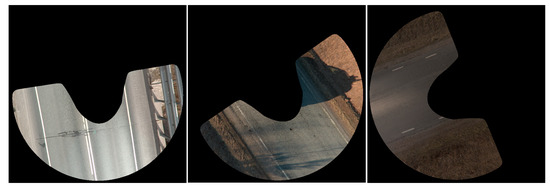
Figure 1.
The orthoframes depicting the road.
For each orthoframe, an U-shaped mask has been supplied and applied that eliminates less relevant (unfocused, distorted) parts of the orthoframe. Each orthoframe is accompanied with a VRT file. VRT files are used within and are essentially XML files containing metadata that describe various properties of the associated raster image. For present case, VRT files provide the geolocation coordinates of the upper left corner of the orthoframe as well as pixel dimensions, making it possible to compute exact geolocation coordinate for each pixel in the orthoframe, if necessary.
There is also an existing defect layer, catalogued by Teede Tehnokeskus Ltd [23] and provided in a set of files that can be parsed using Python Shapefile library and contains information about the pavement defects based on general polyline, polygon, or point defect types. The defect shapes and coordinates in the base defect layer (BDL) are often not very accurately specified as this is not critical in the application in which they were used originally and thus not the primary concern of the original digitizers. We would not be able to use this information for training the ConvNets, however, BDL helps us to choose the orthoframes for detailed annotation and training throughout active learning.
While there are a number of different defect types present in the source data (such as cracking, weathering and potholes), we do not separate them into different classes due to class imbalance, as there would be insufficient data for the ConvNets to distinguish between the classes. However, in contrast with our previous work [12], we now digitize all classes of defects, not only cracks.
It has been observed [12] that due to simple laws of optics, road surface in these orthoframes gradually loses detail as the distance from the original camera shooting location increases, therefore regions further from the camera lack sufficient detail to properly distinguish the features of the road. We extract the more detailed part of the orthoframe by using a mask that is obtained by multiplying the original orthoframe mask with a filled circle with a radius of 1500 pixels.
Ignoring a portion of the orthoframe does not present a problem as the orthoframes are shot frequently (at every 3 distance) and partially overlap, except for the edges for which we need to extend the mask. This is accomplished by adding a rectangle covering the upper part of road in the orthoframe to the mask production formula (Figure 2).

Figure 2.
Generation of the region-of-interest orthoframe mask.
3. System Configuration
The aim of this research is to develop a ConvNet based pavement distress detection system (PDDS) that is able to automatically generate a mask of defective road areas for a given orthoframe. However, we must first note that the orthoframe is an RGB image of resolution 4096 × 4096 pixels, which due to GPU memory limitations is too large to feed to a single ConvNet as an input, especially considering that better results are achieved by training the ConvNet with a batch size of 8 to 64 [24]. To tackle this issue, the proposed system operates in three stages, using three separate ConvNets:
- Road Segmentation Network (RSN) is a U-Net inspired ConvNet that generates a road area mask for the orthoframe so that the parts of the orthoframe where pavement defects cannot exist are explicitly eliminated. The network operates on orthoframes cut and resized to 512 × 512 pixels. The masks are restored to the original size, after the prediction is made by the network.
- Defect detection network (DDN), a classification ConvNet that assigns a binary classification (defective/non-defective) to each of 224 × 224-pixel patches sampled from the area of the orthoframe belonging to the predicted road area mask.
- Defect Segmentation Network (DSN), another U-Net based ConvNet, is applied to generate pixel level segmentation for all the patches belonging to the defective category. The 4096 × 4096-pixel defect mask is constructed by arranging the patches back together.
The workflow is illustrated in Figure 3. In addition to the defect segmentation mask, the system computes the real-world coordinates of the patches categorized as defective using the corresponding VRT file accompanying each orthoframe in the dataset.
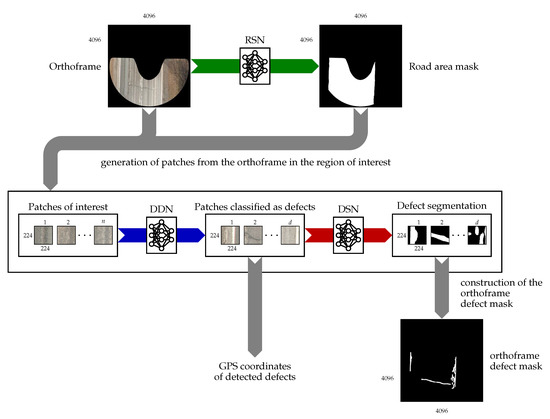
Figure 3.
Overview of the inference process for defect segmentation over an orthoframe.
4. Road Area Extraction
4.1. Architecture
Road area extraction (RAE) is necessary in order to define the region of interest (ROI) and is performed by RSN which is a ConvNet inspired by U-Net [25] architecture (Figure 4).
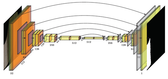
Figure 4.
Illustration of Road Segmentation Network (RSN) architecture.
The RSN consists of five encoding blocks, five decoding blocks, a final segmentation block and shortcut connections between the encoding and decoding blocks. Each encoding block consists of six layers—(1) a batch normalization layer, (2) first convolutional layer, (3) first LeakyReLU activation, (4) second convolutional layer, (5) second LeakyReLU activation and (6) a max pooling layer. The decoding blocks have a similar structure except that max pooling layer is replaced with upsampling layer which is followed by a concatenation layer, thus an encoding block consists of seven layers. Encoding blocks have two outputs: (1) feature maps after max pooling connected to the next block and (2) feature maps before max pooling connected to the corresponding decoding block concatenation layer. The final segmentation block has only two layers—(1) a batch normalization layer and (2) a convolutional layer. Within a block, each convolutional layer has the same number of convolutional kernels, but not all blocks have the same number of kernels. However, an encoding block and its corresponding decoding block have the same number of convolutional kernels. Thus the first encoding and the last decoding block have 32 convolutional kernels. In the next encoding block the number of kernels is doubled (64) until it reaches 512 in the last encoding block. In contrast, the segmentation block’s convolutional layer only has a single kernel.
4.2. Data Processing
In order to avoid excessive resource usage, the original images (orthoframes) are (i) rotated so that the longest side of the U-shaped colored area of an image is orthogonal to the y-axis, (ii) the upper part of orthoframe that does not contain any colored pixels is cut off, (iii) the resulting images are split into two halves along the y-axis and one of two images is flipped over the y-axis (this ensures that the road area is mostly located on the left side of the image), (iv) both of the halves are padded with black pixels on the side in order to have a square image, and (v) the image is resized to 512 × 512 pixels. The same operations are concurrently performed on the annotated road area masks (Figure 5).
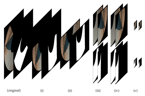
Figure 5.
Road area image pre-processing.
On the resulting predictions, the same operations are performed in the reverse order. That is, the predictions are up-scaled, excess width is removed, one half is flipped over the y-axis, both halves are combined, the empty/black upper part is added—the image now has its original size—and, finally, the mask is de-rotated.
5. Defect Detection
In order to locate areas likeliest to contain defects within the previously generated road area mask of the orthoframe, we use a ConvNet based binary classifier that will be referred to as the Defect Detection Network (Defect Detection Network (DDN)). As opposed to a segmentation ConvNet, a classification ConvNet produces only a single label for a processed input, which in our case can be “defective” or “non-defective”. To ensure some degree of localization for the proposed defects, the relevant area of the orthoframe is first partitioned into patches of size 224 × 224, each of which are subject to classification.
5.1. Architecture
Given the complexity of the task due to non-uniform illumination, inconsistent image sharpness, varying road conditions, patches partially including the side of the road and so forth., a deeper ConvNet architecture is necessary than for RSN. In our previous research [12], a ResNet based on transfer learning [26] architecture was found to attain satisfactory results for situations in which the patches were sampled from roads with less ambiguous defects and better lighting conditions. However, our further developments on similar datasets have shown that there is a possibility of obtaining slight performance gains by utilizing the contextual area surrounding each of the patches within the orthoframe [27]. By extracting relevant features from not only the patch but also its surroundings, we can train a classifier better equipped to deal with difficult cases in which more contextual information is needed for an accurate classification (such as when a pavement crack lies at the very edge of the patch).
In order to extract helpful contextual features to the ConvNet, our approach is to introduce an auxiliary input stream for the feature extraction part of the network. Thus, the ConvNet operates with content-context input pairs in which the classification label is determined solely by the content input. An illustration of how this pair is extracted from an orthoframe is given in Figure 6.
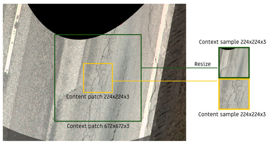
Figure 6.
Extraction of a content-context sample from an orthoframe.
The extracted features are then flattened and concatenated to attain a fully connected layer of length 8192, with the content and context streams contributing an equal amount of neurons to the layer. These neurons, each with their respective weights, are then fed to an additional fully connected layer of 1024 neurons. Finally, these 1024 neurons are connected to 2 output neurons, representing the classes of “defective” or “non-defective” and softmax function is applied to get the network’s probability distributions for the given input pair. For the feature extraction part of the architecture, ResNet models pretrained on the ImageNet [28] dataset are used as this approach has been demonstrated to result in faster convergence during training [29]. Pretrained ResNet architectures come in many depths but we chose the 34-layer one in an effort to find balance between performance and inference speed, as the defect detection part of the PDDS tends to be the bottleneck in terms of speed. A condensed scheme of the described two-stream classification network can be seen in Figure 7.
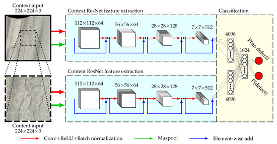
Figure 7.
Architecture of the defect detection convolutional neural network (ConvNet) used in this work.
6. Defect Segmentation
The last of three models of the proposed system is the Defect Segmentation Network (Defect Segmentation Network (DSN)), which produces pixel-wise predictions of defective regions for a given patch. With this approach, we are able to visualize contours of potential defects in an image, not only the patches the defects were detected in. This in turn increases the system’s interpretability and usefulness, as it is required by Estonian road administration to detect pavement defects with pixel-wise localization in order to better calculate the distress on a given road.
Architecture
Just like RSN, DSN is inspired by the U-Net autoencoder architecture (described in Section 4). However, for this particular task, deeper architectures are experimented with, as the defect segmentation part of PDDS is most prone to error. In addition, the segmentation model can afford longer computation times since this model is only invoked for patches that have been classified as defects, making it less likely to become the bottleneck of the system (most patches are non-defective).
Given the flexibility of the U-Net approach, it can be used with a variety of different encoders, as will be demonstrated in Section 10.2.3. While various encoders were experimented with, the decoder part of the architecture remained constant for each model. The decoder consists of 5 layers of decoder blocks, where each block first upscales the input channels by a factor of two and then performs two Conv3x3-BatchNorm-ReLU operations sequentially. For each consequent decoder block, the number of output channels is halved, so the first layer has 256 output channels and the fifth layer has 16 output channels. As the encoder channels of matching resolutions get concatenated for the first four decoder blocks in order to preserve features, the total number of input channels per block is higher than the output channels in the preceding decoder layer. In Figure 8, a DSN U-Net architecture with a ResNet backbone is illustrated.
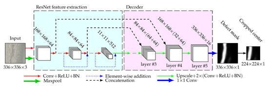
Figure 8.
Architecture of the defect segmentation U-Net used in this work.
The defect segmentation model predicts over inputs of size 336 × 336, as opposed to the patch input size of 224 × 224. This is done to provide supplementary context around a given patch, from which potentially useful features could be extracted. The necessity for this approach was noted when the reconstruction of the 4096 × 4096 orthoframe defect mask resulted in defect contours that were discontinuous, due to the low confidence the model provides at the edge of the input. Therefore, we now discard the outputs that are outside the central 224 × 224 area of the prediction mask, as predictions in that ribbon are of a lower quality.
7. Performance Metrics
In the ideal world, all instances of pavement defects can be found and localized. In the real world, however, the system may miss the existing defects and detect non-existing ones for a number of reasons (lighting, surface condition, image quality issues, etc.). The accuracy of detecting the defects needs to be determined in the most appropriate manner.
PDDS consists of three prediction networks, each of which can provide erroneous predictions that propagate to the next network. For example, if road area is incorrectly determined by RSN (say, smaller than it properly should be), all the defects that are in the area improperly classified as “not road” cannot be identified. Similarly, if DDN fails to recognize a defect in a patch, this patch is never sent to DSN and goes unnoticed.
7.1. Pixel-Level IoU, Precision and Recall
Two of three networks in the system are semantic segmentation networks and the output of the system also consists of semantically segmented images. Semantic segmentation tasks are usually evaluated by Jaccard similarity index, also known as IoU (intersection over union)
where TP stands for number of pixels correctly predicted to belong to a given class, TN for number of pixels correctly predicted not to belong to a given class, FP for number of pixels falsely predicted to belong to a given class, and FN for number of pixels falsely predicted not to belong to a given class. IoU is the area of overlap between the ground truth (X) and the predicted semantic segmentation (Y) divided by the area of union between the predicted semantic segmentation and the ground truth. Note that
7.2. Instance-Level IoU
It is well-known that the global IoU measure (1) is biased toward object instances that cover a large image area. This becomes troublesome in applications where there is a strong scale variation among instances and pavement distress detection is definitely one of such applications. To address the issue, an instance-level intersection over union (iIoU) metric has been proposed [30]
where iTP, iFN denote the numbers of True Positive and False Negative pixels per i-th instance, respectively, weighted by where is the average instance size. The False Positive pixels, however, are not associated with any instance and thus do not require normalization.
The iIoU aims to evaluate how well the individual instances in the scene are represented in the labeling, however, if iIoU < IoU, it simply means that smaller objects are not detected with the same accuracy than larger objects and vice versa.
For example, Figure 9a depicts a fragment of an orthoframe in which there are two ground truth instances (one of which is predicted well and another poorly) and one false prediction. The distribution of pixels is as follows TP = 35,567, FP = 10,658, FN = 14,449, which yields 59% global IoU (1). When calculating iIoU, iTP = 34,699, iFN = 548, iTP = 868, iFN = 13,901 thus = (iTP+ iFN+iTP+iFN)/2 = 25,008, , , which yields 43% iIoU. iIoU is considerably smaller than IoU because the instance which gives most True Positives is larger than and the instance that yields most False Negatives is smaller than .
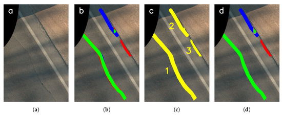
Figure 9.
An illustration of various metrics. (a) The original image; (b) TP, FN and FP pixels are depicted by colors of green, blue and red, respectively; (c) Three objects obtained by combining the predictions and ground truth instances; (d) TP, FN and FP pixels with edge-tolerant intersection over union (IoU) computation.
7.3. Object-Level IoU
To truly assess how well individual instances are represented in the labeling, one needs to look further from ground truth instances. We propose to combine ground truth and prediction pixels, X and Y to obtain objects (Figure 9c). A given object consisting of prediction and ground truth pixels can contain any combination of number of pixels correctly predicted to belong to a given class (TP), number of pixels falsely predicted to belong to a given class (FP) and number of pixels falsely predicted not to belong to a given class (FN) pixels. In the referred image, object no. 1 consists mostly of TP pixels, object no. 2 mostly of FN pixels and object no. 3 contains only FP pixels.
To compute intersections over unions (IoUs) for each object we need to define object-specific TP, FP and FN pixels as follows
where and are ground truth and prediction pixels belonging to the j-th object,
and computation of object-level intersection over union (oIoU) for an j-th object is straightforward
For the considered example, oIoU, oIoU, oIoU, which matches well with what we see in Figure 9b.
7.4. Edge-Tolerant IoU
One very specific characteristic of pavement distress detection is that the defects (the cracks in particular) can be highly irregular and are made up of lines of small diameter. Annotating every little detail of such defect with a sharp pen is too time-consuming for practical purposes. An annotation is therefore often a rough sketch of the annotated defect and contains a substantial amount of perfectly fine road surface. This also means that minor detection mismatches at the edges of a detected defect are not necessarily mistakes at all, neither are they critical to the success of the application. Moreover, they can bias the evaluation measure in the undesired direction.
To account for that we propose an edge-tolerant object-level IoU—a more complicated approach than the one taken in References [10,31,32] where a true positive is simply defined as any labelled pixel in the output segmentation mask that is within 5 pixels of a true label in the ground truth—in which object-level FN and FP pixels are calculated as follows.
where is a dilated ground truth instance belonging to the j-th object (using a fixed-size kernel) and is a similarly dilated set of prediction pixels belonging to the same object.
An edge-tolerant object-level IoU would appear as
and global edge-tolerant intersection over union (eIoU)as
In the example, having the kernel size of 7 pixels, it would mean that eIoU, eIoU, eIoU and the overall IoU, eIoU = 66%. We can see (Figure 9d) that the only truly affected object by this is object no. 1, which was the original purpose.
7.5. Classification Performance Evaluation
Much like in semantic segmentation, there are four possibilities concerning the judgments of road patches provided by DDN:
- true negative—there is no defect and the system does not detect a defect;
- true positive—there is a defect and the system correctly detects it;
- false negative—there is a defect, but the system does not detect it
- false positive—there is no defect, but the system detects a defect.
If number of pixels correctly predicted not to belong to a given class (TN), TP, FN, and FP denote the total counts of corresponding detection outcomes, it is possible to calculate classification precision and recall applying the formulas (3) and (4).
In addition, Matthews correlation coefficient (MCC) metric, defined as
provides a reliable measure in case of imbalanced data.
7.6. Estimating the Number of Detected Defects
In applications like this, one also needs a basic measure, simple enough to understand, how accurate the system is. Such measure can tell us, for example, how many defects of all defects were detected with sufficient accuracy.
In object detection, it is common to calculate IoU for predicted and ground truth instance bounding boxes. A prediction is considered correct if the IoU of the predicted and ground truth bounding boxes exceeds some threshold (typically 0.5) [33].
Inspired by this, we use the measures of object-level precision (15) and recall (16) to determine if an object represents a true positive, false positive or false negative prediction.
Given a threshold (for example, = 0.5), there are six possibilities (Figure 10)
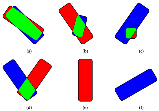
Figure 10.
Classification of segmented defects. As in Figure 9, colors green, blue and red depict TP, FN and FP pixels, respectively. (a) true positive; (b) false positive; (c) false negative; (d) false negative and false positive; (e) false positive; (f) false negative;
8. Annotation Procedure
As noted in Section 2, it is not possible to use the information in BDL for automatic annotation of the orthoframes. We have developed a fast and easy-to-use labeling tool to annotate the existing defects as well as road contours so as to produce the training data.
The tool, from the implementation perspective, is built using Python 3 with the PyQt5 [34] framework for building the graphical user interface. The choice of programming language is justified by the fact that it makes developing the project streamlined because we use Python for all other tasks such as image processing and deep learning. The packages developed for these tasks can thus be easily integrated into the present application. The simplified class and package relationship is shown in Figure 11.
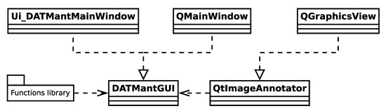
Figure 11.
Simplified UML diagram of the class and package relationships making up the DATM annotation tool.
The three major components lie on the second row of the diagram. We now briefly describe the functionality of each component.
8.1. Functions Library
The functions library provides two main tools:
- Support for generating tighter masks that help the annotation process by shading the less sharp parts of the orthoframe (considered to be outlying parts) darker.
- Drawing pre-made annotations for defects, if this information is available in shapefile format.
These functions are not critical to the application, but are of help to the personnel engaged in annotating the orthoframes.
8.2. DATMant Graphical User Interface
This is the main component of the application that implements the annotation workflow described in this manuscript. In this sense, the tool is specific to this concrete workflow. The idea is to walk the folder in the operating system containing the orthoframes providing two annotation layers for each orthoframe:
- Defects layer—positive in-painting—paint is applied over defects detected on the orthoframe. At this stage any defect as marked as such without specifying the type of defect.
- Road area layer—negative in-painting—paint is applied on outlying area that does not contain pavement. This layer is used for other image processing related applications.
Both layers are saved as binary image masks to the orthoframe folder following a certain file naming convention. The tool automatically checks whether updated masks already exist in that folder and loads those masks, if they do.
With respect to defect masks—if an updated mask is not available, but a ConvNet-generated one is, the tool will load the latter as a starting point for the annotation process.
Furthermore, the tools described in Section 8.1 are also applied as needed to allow the person doing the annotation to see the area where defects should be in-painted and show the defects also, if they are supplied.
The process of annotating defects on zoomed-in part of the orthoframe is shown in Figure 12.
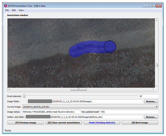
Figure 12.
Graphical user interface of the annotation tool written in Python 3 with the PyQt framework.
8.3. QtImageAnnotator Component
From the perspective of workflow, this is a critical component, since it must support a flexible and rapid workflow. The component itself is implemented as a QGraphicsScene which means it can be embedded into any PyQt5 based application. The remarkable property of this component is that its functions for interactions are implemented inside it so it works as a drop-in component.
The main goal of using this component is to implement the binary mask annotation procedure. An image (in case of this work, an orthoframe) is loaded as background and the user must then in-paint the mask over interesting features. The mask is semi-transparent and is displayed as an overlay in the viewport.
The following additional features are implemented to ensure the workflow is efficient and flexible:
- Easy zoom-in and zoom-out features and mouse navigation.
- Ability to temporary hide the mask overlay to check the image underneath.
- Line segment insertion—the user must hold the Shift key to create line segments.
- Flood-fill technique [35] for easily creating filled regions. In this particular application, this is especially useful for road area mask creation when coupled with line segment insertion.
- Undo functionality supporting undoing all in-painting actions. Every time an image is loaded, the undo buffer is initialized with a maximum of N states (can be changed by the user depending on the available memory in the annotation device).
The parameters of the component like paint color and brush size can be changed by the hosting application. In case of the tool described in Section 8.2, the choice of brush size is integrated as a slider into the user interface. The paint color is determined by the user as well, in this particular case, the color blue is used to paint over defects, while the color red is used to mask away parts of the orthoframe without actual pavement.
8.4. Tool Availability
The annotation tool is released as open source software [36]. While the base UI may not be directly applicable to other projects without significant modification, the QtImageAnnotator class can work as a drop-in component having the functionality discussed above.
9. Active Learning of Pavement Defects and Road Contours
ConvNets have been shown to be successful in many tasks but there is a major drawback as typically a large amount of labeled data is necessary to learn the large number of ConvNet parameters. The dataset must be comprehensive as well as diverse as this is essential for training accurate and well-generalizing neural networks, especially when visual appearance of objects of interest and background varies considerably.
It is almost always better to have more training data since the accuracy and higher representative power is dependent on that but labeling a dataset is a time-consuming and therefore also an expensive task. On the other hand, data samples are not equal in the sense that some are able to contribute more to the training of the network than others and it would make sense to prefer such data samples that are able to maximize the network performance.
This can be addressed by active learning, an iterative process in which a model is learned at each iteration and a subset of data is chosen to be labeled from a pool of unlabeled data ranked for their automatic selection by some measure of informativeness [37].
Most often such measure in active learning is based on uncertainty but it has been argued [38] that choosing to annotate the unlabeled samples which lead to predictions with lowest confidence is not an efficient active learning criterion for ConvNets. We opted to use the information in the BDL and select the images that would yield the highest number of false-positive and false-negative predictions by the PDDS in respect to the BDL.
It is, however, observed that the number of defects detected by the digitizers of the BDL is about two times lower than the number of defects detected and annotated by the digitizers who annotated the orthoframes for RSN/DDN/DSN training. This means that even if PDDS performs perfectly, the number of false positives in respect to BDL would be large and thus the measures of precision (3) and IoU (1) are not helpful.
The solution is to use recall (4) for trailing the orthoframes where PDDS makes the most false negative predictions and the orthoframes that yield the most false positives are sought among the orthoframes where the number of BDL defects is zero.
Consequently, for each orthoframe, passed through PDDS, first we determine the value of recall. If this appears to be larger than zero, the value of recall is directly used as the ranking value to choose the orthoframes to the annotation pool—orthoframes having the lowest ranking value are chosen first.
In case recall equals zero (indicating that BDL defects do not exist), we calculate the total area of predicted defects S in the orthoframe and divide it by the total area of the orthoframe . The ranking value is calculated by so that the more meaningful orthoframes are, again, represented by a lower ranking value.
These rankings cannot be combined, so, empirically, for each orthoframe picked after the predicted defects area (to improve performance on false positives) we take two orthoframes picked after the recall value (to improve performance on false negatives).
The whole active learning workflow is depicted in Figure 13. Note that the PDDS output, even if it contains mistakes, can be passed to digitizers as initial annotation and can thus speed up the annotation process.
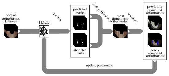
Figure 13.
Active learning of road contours and pavement defects.
10. Experiments and Results
10.1. Datasets
By the time of writing, the dataset is comprised of 6789 orthoframes annotated for defects and road areas, all captured from Estonian roads over the past 2 years. Of these orthoframes, 947 have been reserved for testing, in order to measure the performance of the system. Using the tool described in Section 8, the defects were annotated with a minimum brush diameter of 40 pixels in order to speed up the procedure. Therefore, the attained ground truth masks of defects are coarse.
To get the most meaningful test set, that is, one that would correlate with scenarios that the system would encounter in deployment, the majority of the test set (533 orthoframes) is comprised of a road from which none of the orthoframes were used for generating training samples. This defect-ridden strip of road is also used by Estonian road administration to evaluate the performance of human digitizers. However, given the lack of diverse scenarios from just a single road amounting to about , additional orthoframes from 3 other roads (414 in total) were used for testing. In an effort to minimize potential overlap between testing and training datasets, orthoframes belonging to the latter part of the road capturing session were added to the test set, while the earlier orthoframes were reserved for training and validation.
In addition to the full dataset, a smaller dataset containing of 200 randomly sampled orthoframes was used to verify the feasibility of different network architectures and hyperparameters with less computational resources.
Data Sampling
For DDN and DSN, samples are generated across the training set with half-step sliding windows of size 224 × 224 and 336 × 336 respectively. For each DDN sample, the 672 × 672 area surrounding the sample is also captured and resized to 224 × 224 in order to generate inputs for the context feature extractors of the DDN as described in Section 5.1. Given that parts of an orthoframe do not depict the road, the samples are only generated from areas that have been annotated to be part of the road. However, to increase robustness and coverage, samples partially out of this area (road edges) are also included. The classification label of a sample is “defective” if at least 5% of the pixels in the sample are defective.
For the DDN and DSN, three different sampling strategies were considered (visualized in Figure 14):
Figure 14.
Three of the sampling strategies visualized on an orthoframe. Each green square is of size 336 × 336 and added to the given dataset. For illustrative purposes, annotated defects are marked in blue and predicted false positives (only shown in c) are marked in red. For the sake of visual clarity, partial overlapping is not displayed and the focused part of the road in conjunction with the road area mask is highlighted. (a) Full sampling.; (b) Dilated defect contour sampling.; (c) Defect contour sampling with false positives.
- Full sampling—all possible patches are sampled from each orthoframe and added to the training set. This sampling strategy is used for the DDN training. However, it would not be favorable to sample all patches for the DSN because during deployment it is expected to predict over patches that are already likely to contain defects. Therefore, during training a similar class imbalance distribution should be present. Nonetheless, experiments were later performed to confirm this theory with the 200 orthoframe dataset as seen in Section 10.3.
- Dilated defect contour sampling—patches that include contours of annotated defects are sampled from, as well as areas surrounding these contours.
- Defect contour sampling with false positives—first, predictions are made across the entire training and validation orthoframes with the latest model. Then, patches where false positives occurred are added to the training and validation datasets, in addition to the patches that were annotated to be defective.
The sample count and class distribution for each considered dataset can be seen in Table 1.

Table 1.
The datasets used in this work, generated from the orthoframes reserved for training and validation.
10.2. Training
10.2.1. RSN Training
The RSN was trained and tested in multiple iterations as more annotated orthoframes became available. Each training iteration was performed from scratch to avoid using images that were in the training dataset in the previous iteration in the validation dataset in the current iteration. During the training, additional data augmentation is applied to these images: (1) horizontal and (2) vertical flipping, (3) shifting and (4) rotation. The augmented images are processed in batches of eight and model parameters are updated after each batch in respect to the gradients backpropagated from IoU loss (18).
where is the IoU loss, K is the set of all pixels in the images in the batch, is the label for the given pixel and is the predicted probability for the correct label of that pixel. Note that while cross entropy is the de facto default loss function for classification, object detection and semantic segmentation tasks, it is mathematically much more closer to accuracy—that is biased toward reporting the accuracy of identifying negative cases—than IoU, even though the final performance of semantic segmentation models is measured using IoU [39,40].
The RSN model uses Adam optimizer with initial learning rate (LR) of 1 × 10. The LR was halved if validation loss did not improve in 18 epochs. The final version of RSN was trained in 79 epochs.
10.2.2. DDN Training
Training of the DDN model follows the mini-batch gradient descent protocol: the input samples are processed in batches of 64 and model parameters are updated after each batch with respect to the gradients backpropagated from the cross-entropy loss, which is defined as follows:
where is the cross-entropy loss, K is the set of patches in the batch, is the label for the given patch (non-defective/defective) and is the predicted probability of the patch being defective.
Since the models are updated iteratively, the weights are initialized according to the best performing model of the previous iteration, in order to speed up training. For the first iteration, the weights optimized for the ImageNet dataset were used. Learning rate (LR) scheduler for the DDN from scratch uses the 1 cycle learning rate policy, which has been shown to speed up ConvNet training [41]: for the first 10% of the training process, the LR rises from 4 × 10 to the maximum learning rate of 1 × 10, after which it gradually drops to the lowest learning rate of 1 × 10. Base and maximum momentums were set to 0.85 and 0.95, respectively. This policy was implemented using the LR scheduler OneCycleLR provided by PyTorch [42]. The learning rate policy for the following iterations was performed with the step decay learning scheduler, where the learning rate linearly decays from 5 × 10 (first epoch) to 1 × 10 (last epoch), which was also provided by PyTorch (StepLR). The Adam [43] optimization algorithm was used for updating parameters per batch. Given the relatively large number of partially overlapping training and validation patches (814,426), the model for each iteration is trained only for 4 epochs. To attain more robust models, data augmentation is used for each sample with random flipping, rotation, Gaussian noise, Gaussian blur, brightness adjustment, contrast adjustment and RGB value shifting, all provided by the Albumentations library [44]. Lastly, as DDN computes probabilities and not discrete values, which is needed for the DSN, we choose the threshold such that on the validation set.
10.2.3. DSN Training
As with the DDN model, the DSN is also trained with the mini-batch gradient descent protocol, however, a batch size of 16 instead of 64 is used, due to GPU memory being more limited by the larger input size of 336 × 336 × 3. Similarly with RSN training, the IoU loss function (18) is used for the later models (Iterations 4 and 5) and the pixel-wise cross-entropy loss (19) is used for the first three iterations. Encoder weights for the model are initialized from the previous iteration or from ImageNet if no such architecture was trained in the previous iterations. As with the DDN model, training the DSN model follows the 1cycle policy with Adam optimizer and hyperparameters as specified in Section 10.2.2. Additionally, the augmentations used in Section 10.2.2 are also used for the samples processed during DSN training. For each iteration the DSN model is trained for 25 epochs.
10.3. DSN Architecture, Data Sampling and Patch Size Experiments
With the flexibility of the U-Net approach, most ConvNet encoders can be used as the backbone for our DSN model. Many different pretrained ConvNets have been made publicly available, most notably models pretrained on the ImageNet competition [28]. While models that perform well on ImageNet generally do well on other datasets [29], this has not yet been verified for pavement distress related tasks. Thus, in an effort to search for the best performing encoder for our task, we evaluated a variety of pretrained encoders that have previously shown good results on the ImageNet dataset.
The experiments were conducted on the 200 orthoframe dataset over 40 epochs, with 2-fold cross-validation. The encoders evaluated, provided by Reference [45], include ResNet34 [26], ResNet50 [26], SE-ResNet50 [46], Inception-v4 [47] and DenseNet-121 [48]. The training protocol for each model followed the one described in Section 10.2.3.
From the results displayed in Figure 15, it can be seen that the Inception-v4 model outperforms other models both in terms of validation and training IoU. Therefore, we will proceed with this architecture in the future.
Figure 15.
Defect Segmentation Network (DSN) results for different encoder architectures over 40 epochs trained on the 200 orthoframe dataset. Performed with 2-fold cross-validation.
To evaluate data sampling and patch size options that should be used with the full dataset, experiments presented in Table 2 were conducted on the 200 orthoframe datasets by training the DDN and DSN models with ResNet34 backbones for both. The DDN was trained on the full sampling strategy for each experiment that used a DDN. For result evaluation in Table 2, ground truths were used for road area detection.
Table 2.
Test set IoUs for different patch sizes and data sampling strategies on the reduced training set.
Evidently, the DDN adds a lot of performance to the system, as the segmentation network alone trained with the full sampling strategy performs worse than systems using the DDN pipeline. The advantages of the “classification before segmentation” approach has also been noticed by other researchers [49].
The difference between sampling strategies (2*) and (3*) seems negligible. While sampling strategy 1 achieved similar results when combined with a DDN, it was trained on nearly 3 times the amount of samples and the same amount of epochs. Thus, (1*) will be considered as an inefficient sampling strategy for the DSN and further experiments will proceed with sampling strategy (3*). With regards to the patch size, performance gains can be noticed by adding more context to the patch and cropping the central part. However, it seems that adding context past the size of 336 × 336 is unnecessary. Different levels of context for a patch are visualized in Figure 16.
Figure 16.
Visualization of the context captured for different DSN patch sizes. For models with input sizes of 336 × 336 or 448 × 448, the output gets cropped to the central part of size 224 × 224. In each case, the orthoframe still gets partitioned into patches of size 224 × 224, which are shown as yellow squares.
10.4. Performance and Evaluation
In order to measure progress throughout different annotation and training cycles, as specified in Section 9, we provide a variety of metrics monitored for each specific iteration in Table 3. It should be mentioned that the DSN metrics are computed over the orthoframes of size 4096 × 4096, not just the given patches. Thus, errors made by the RSN and DDN are propagated and result in a lower DSN IoU value. Examples include scenarios in which the RSN failed to capture a part of the road or if the DDN failed to detect a defect (or detected false positives which the DSN struggled with). For eIoU, the metrics were calculated with a tolerance diameter radius of 7 pixels, as the annotations were done with a 20 pixel radius brush.
Table 3.
Defect segmentation performances computed over the test set. Iterations with their respective number of training and validation orthoframes are specified.
Additionally, DDN and RSN performances over iterations are provided in Table 4 and Table 5 respectively.
Table 4.
Defect detection metrics for the test set over iterations.
Table 5.
Road area segmentation metrics for the test set over iterations.
It can be noted that a significant performance boost was gained from iteration 2. One possible explanation for this is that during iteration 1 we had not yet deployed the active learning approach (described in Section 9) for selecting new orthoframes to annotate. However, for the few following iterations, the performance gains seem to have halted. Perhaps this could indicate that the amount of orthoframes annotated for training is already sufficient and the models have reached their limits. It is also worth noting that we select only the most difficult orthoframes for the model to annotate. Thus, the static test set might not cover many of the edge cases where the model might underperform significantly, so the model’s increase in robustness to a variety of scenarios might not be fully reflected in these experiments. In iteration 5, another leap in performance was noticed, which is likely due to the improved DSN architecture. Another curious detail to note is the comparatively high iIoU value for iteration 1. This can be traced to the fact that 533 of the test set images were already annotated on the basis of the outputs of iteration 1.
To measure the DSN performance loss attributable to the errors propagated from the RSN and DDN models, we provide the results of another experiment in which the RSN and DDN models were replaced with ground truths in Table 6.
Table 6.
Defect segmentation performances computed over the test set, where Road Segmentation Network (RSN) and Defect Detection Network (DDN) networks are replaced with ground truths.
Comparing the results from Table 3 and Table 6, the DSN IoU reduction due to RSN and DDN is 9.3%. However, for cPr and cRc, the reduction is 25.5% and 12.1% respectively. This indicates that many falsely detected contours can be reduced by increasing the precision of the DDN. Additionally, it shows that many of the errors made by the combination of RSN and DDN are due to defects being detected only partially, as a defective contour can span across multiple patches in a given orthoframe. The fact that the drop in iIoU (12.2%) is greater than the drop in IoU (9.3%) indicates the smaller defects are the ones that the DDN struggles the most with.
Outputs from the system with varying levels of success are displayed in Figure 17. Keeping in mind the average IoU across the entire testset is 0.515, we see in the more successful output Figure 17a that the PDDS is capable of localizing and segmenting crack defects across the entire orthoframe, without causing suffering from false positives from various contrastive line formations found on the road. In Figure 17b, another example is shown in which a longitudinal crack is well segmented despite poor illumination in the given orthoframe. Additionally, we see the benefits of using the eIoU metric, as the seemingly ideal result only produces a pixel-wise IoU of 0.79 but an eIoU of above 0.99. Figure 17c shows a number of false positives across the orthoframe, including one road marking in the middle of the road, a patch that is mistaken for weathering and various formations at the right side of the road. Additionally, the road area segmentation task is made harder by the crossroad. In Figure 17d, we see sharp shadows across the orthoframe, which do not generate false positives on their own. However, despite the well segmented alligator cracking, the right road edge suffers from false negatives and false positives, which might be partly due to the image being blurrier in that part of the image.
Figure 17.
Orthoframes from the test set processed by the PDDS . RSN outputs multiplied by the region of interest mask are highlighted. Patches classified by the DDN as non-defective have white borders and patches classified as defective have red borders. For the masks produced by DSN, the green, red and blue contours represent true positive, false positive and false negative pixels respectively. (a) IoU = 0.846, eIoU = 0.930, iIoU = 0.457, cPr = 0.600, cRc = 0.750; (b) IoU = 0.790, eIoU = 0.991, iIoU = 0.582, cPr = 1, cRc = 1; (c) IoU = 0.104, eIoU = 0.110, iIoU = 0.306, cPr = 0.143, cRc = 1; (d) IoU = 0.515, eIoU = 0.575, iIoU = 0.306, cPr = 0.750, cRc = 0.500.
Lastly, as the system is comprised of three models of around 100 million parameters in total and there are thousands of kilometers of roads to cover, we must consider the inference speed as an important performance metric. In Table 7, inference speed averages over the test set are provided. These experiments were conducted on a Windows 7 PC with an Intel i7-7700 CPU, 16 GB of RAM and a GeForce GTX 1080 GPU. Note, however, that multiprocessing was not used in these experiments, so further optimizations are possible. For the test set, there are on average about 63 patches per orthoframe and on average 11 of them get detected as defective. Thus, the DDN takes 33 per patch and the ResNet34 and Inception-v4 networks take 59 and 79 per patch, respectively. As the average orthoframe covers around 3 of road in length, the processing speed is about .
Table 7.
PDDS inference speed, separated by different modules of the pipeline. For each column, the seconds taken per orthoframe is shown.
11. Conclusions
Transportation infrastructure systems are essential to the government and commerce. Camera-based pavement distress detection plays a critical role in pavement maintenance and rehabilitation and early detection of distresses developing in pavements offers significant cost savings resulting from timely maintenance and repair.
Automated detection of distresses from pavement images is, however, a challenging problem due to a number of factors—variations in image quality, non-uniformity of cracks and surface texture, lack of sufficient background illumination, and so forth—which keeps the research community looking for newer and more efficient methods and algorithms. Recent advances in computer vision, largely thanks to the emergence of deep learning, have led researchers to develop robust tools for analyzing pavement images at improved pavement distress detection accuracy.
To address the pavement distress detection problems in Estonia, we have proposed a novel pavement distress detection system that employs three ConvNets and is applied to the orthoframes collected by a mobile mapping system. The first of three networks in the system (RSN) extracts the road area from an orthoframe to be inspected. The second one (DDN) divides the extracted road area into individual patches and labels them into defective and non-defective ones. Third and final network (DSN) segments the defective patches for defects. These networks are expected to operate in a mutually reinforcing manner, however, mistakes that are made by RSN or DDN do propagate through the system. In the end, the defect mask is assembled from segmented patches. The whole process is improved iteratively by active learning.
We have utilized a number of metrics to assess the performance of the system: pixel-wise intersection over union (IoU), edge-tolerant intersection over union (eIoU), instance-level intersection over union (iIoU) and object-level based defect classification precision (cPr) and recall (cRc).
Currently, after 5 iterations of active learning, the PDDS has obtained a pixel-wise IoU of 0.515, eIoU of 0.581, instance-level intersection over union (iIoU) of 0.373, cPr of 0.583 and cRc of 0.641, which have been computed by comparing the 4096 × 4096 ground truth defect masks with the 4096 × 4096 predicted defect masks over the test set. Visual assessment of the produced output indicates that for the majority of orthoframes, the results are satisfactory, despite the complexity of the task.
Each network in the PDDS contributes to the overall performance at a different degree. The analysis shows that road area extraction—easily the most solvable of three subtasks—can be performed with a high IoU above 0.95, whereas recall obtained by the DDN is barely 0.8. We consider recall of the DDN to be more important measure than precision because inability to recognize patches that contain defects means that defects on these patches will never be discovered, much less segmented, whereas inclusion of patches that do not contain any defects still leaves the possibility that the DSN can adequately handle these patches.
Nevertheless, most of the mistakes made by the system can still be contributed to the DSN as segmentation of defects is by nature the most error-prone of three subtasks and further improvements must be sought in this area; by further iterations of active learning and/or by applying more efficient networks/learning schemes.
It should stated, however, that annotation of defects tends to be somewhat subjective, as there is often no visually discernible point where a defect begins and ends. The subjective nature of the ground truth masks is further amplified by the fact that the defects were digitized with a brush diameter of 40 pixels, while cracks, for example, are much thinner than that. It is interesting to note that these factors do not seem to hinder the features learned by our models, indicating that well-performing ConvNets can be achieved on somewhat coarsely annotated training data. However, these factors stemming from subjectivity should be taken into account when monitoring performance metrics, as they might underrepresent the true performance of the system.
While both the DDN and DSN models incorporated contextual features for input processing, there might be additional benefits gained by sharing extracted features across the patches of an orthoframe or between the ConvNets. This could be an opportunity for future research in order to produce more cohesive predictions for the 4096 × 4096 defect masks, as currently the predicted defect contours tend to be fragmented for some of the more difficult orthoframes, due to the sliding window partitioning approach.
The PDDS proposed in this research operates on the same source data, that is, orthoframes, that are used by trained personnel to mark down defects on the road for Estonian Road Administration. The output of our system closely aligns with the goals of Estonian Road Administration for pavement defect inventory. The next challenge in the research is to divide the segmented defects among 11 defect categories, as defined by Estonian Road Administration—transverse cracking, linear cracking, potholes, weathering and so forth. Nonetheless, the PDDS in its current version is already reported to have provided a more efficient workflow for annotators who are able to use it as a baseline to mark down defects, therefore speeding up the process of manual defect annotation.
Author Contributions
Annotation software, A.T.; conceptualization, R.L., R.P. and A.R.; data curation, R.L. and R.P.; formal analysis, A.R.; methodology, R.L., R.P.; investigation, R.L. and A.R.; project administration, A.R.; writing—original draft preparation, R.L., R.P., A.R., A.T.; writing—review and editing, R.L., R.P., A.R., A.T.; visualization, R.L., R.P., A.R.; supervision, A.R.; validation, R.L. All authors have read and agreed to the published version of the manuscript.
Funding
This research endeavor was partially supported by Archimedes Foundation and Reach-U Ltd. in the scope of the smart specialization research and development project #LEP19022: “Applied research for creating a cost-effective interchangeable 3D spatial data infrastructure with survey-grade accuracy”.
Conflicts of Interest
The authors declare no conflict of interest. The funders had no role in the design of the study; in the collection, analyses, or interpretation of data; in the writing of the manuscript, or in the decision to publish the results.
Abbreviations
The following abbreviations are used in this manuscript:
| AI | artificial intelligence |
| BDL | base defect layer |
| ConvNet | convolutional neural network |
| cPr | defect object classification precision |
| cRc | defect object classification recall |
| DDN | defect detection network |
| DL | deep learning |
| DSN | defect segmentation network |
| eIoU | edge-tolerant intersection over union |
| FN | number of pixels falsely predicted not to belong to a given class |
| FP | number of pixels falsely predicted to belong to a given class |
| GDAL | Geospatial Data Abstraction Library |
| iIoU | instance-level intersection over union |
| IoU | intersection over union |
| LR | learning rate |
| MCC | Matthews correlation coefficient |
| MMS | mobile mapping system |
| oIoU | object-level intersection over union |
| PDDS | pavement distress detection system |
| PMS | pavement management system |
| RAE | road area extraction |
| ROI | region of interest |
| RSN | road area segmentation network |
| TN | number of pixels correctly predicted not to belong to a given class |
| TP | number of pixels correctly predicted to belong to a given class |
References
- Ragnoli, A.; De Blasiis, M.R.; Di Benedetto, A. Pavement distress detection methods: A review. Infrastructures 2018, 3, 58. [Google Scholar] [CrossRef]
- Vavrik, W.; Evans, L.; Sargand, S.; Stefanski, J. PCR Evaluation: Considering Transition from Manual to Semi-Automated Pavement Distress Collection and Analysis. 2013. Available online: https://rosap.ntl.bts.gov/view/dot/26795 (accessed on 1 July 2013).
- Mei, Q.; Gül, M. A cost effective solution for pavement crack inspection using cameras and deep neural networks. Constr. Build Mater. 2020, 256, 119397. [Google Scholar] [CrossRef]
- Pan, Y.; Zhang, X.; Cervone, G.; Yang, L. Detection of Asphalt Pavement Potholes and Cracks Based on the Unmanned Aerial Vehicle Multispectral Imagery. IEEE J. Sel. Top. Appl. Earth Obs. Remote Sens. 2018, 11, 3701–3712. [Google Scholar] [CrossRef]
- Yi, L.; Zou, L.; Takahashi, K.; Sato, M. High-Resolution Velocity Analysis Method Using the l-1 Norm Regularized Least-Squares Method for Pavement Inspection. IEEE J. Sel. Top. Appl. Earth Obs. Remote Sens. 2018, 11, 1005–1015. [Google Scholar] [CrossRef]
- Choi, J.; Zhu, L.; Kurosu, H. Detection of Cracks in Paved Road Surface Using Laser Scan Image Data. 2016. Available online: https://pdfs.semanticscholar.org/e591/fcd67903e8c6210a0ec2151ea336536766f9.pdf (accessed on 19 July 2016).
- Bhat, S.; Naik, S.; Gaonkar, M.; Sawant, P.; Aswale, S.; Shetgaonkar, P. A Survey On Road Crack Detection Techniques. In Proceedings of the International Conference on Emerging Trends in Information Technology and Engineering (ic-ETITE), Vellore, India, 24–25 February 2020; pp. 1–6. [Google Scholar]
- Cao, W.; Liu, Q.; He, Z. Review of pavement defect detection methods. IEEE Access 2020, 8, 14531–14544. [Google Scholar] [CrossRef]
- Azhar, K.; Murtaza, F.; Yousaf, M.H.; Habib, H.A. Computer vision based detection and localization of potholes in asphalt pavement images. In Proceedings of the Canadian Conference on Electrical and Computer Engineering, Vancouver, BC, Canada, 15–18 May 2016; pp. 1–5. [Google Scholar] [CrossRef]
- Jenkins, M.D.; Carr, T.A.; Iglesias, M.I.; Buggy, T.; Morison, G. A deep convolutional neural network for semantic pixel-wise segmentation of road and pavement surface cracks. In Proceedings of the 26th European Signal Processing Conference (EUSIPCO), Rome, Italy, 3–7 September 2018; pp. 2120–2124. [Google Scholar] [CrossRef]
- Nie, M.; Wang, K. Pavement Distress Detection Based on Transfer Learning. In Proceedings of the 2018 5th International Conference on Systems and Informatics, Nanjing, China, 10–12 November 2018; pp. 435–439. [Google Scholar] [CrossRef]
- Riid, A.; Lõuk, R.; Pihlak, R.; Tepljakov, A.; Vassiljeva, K. Pavement Distress Detection with Deep Learning Using the Orthoframes Acquired by a Mobile Mapping System. Appl. Sci. 2019, 9, 4829. [Google Scholar] [CrossRef]
- Yusof, N.; Osman, M.; Hussain, Z.; Noor, M.; Ibrahim, A.; Tahir, N.; Abidin, N. Automated Asphalt Pavement Crack Detection and Classification using Deep Convolution Neural Network. In Proceedings of the 2019 9th IEEE International Conference on Control System, Computing and Engineering, Penang, Malaysia, 29 November–1 December 2019; pp. 215–220. [Google Scholar]
- Huyan, J.; Li, W.; Tighe, S.; Xu, Z.; Zhai, J. CrackU-net: A novel deep convolutional neural network for pixelwise pavement crack detection. Struct. Contr. Health Monit. 2020, 27, e2551. [Google Scholar] [CrossRef]
- Sun, M.; Guo, R.; Zhu, J.; Fan, W. Roadway Crack Segmentation Based on an Encoder-decoder Deep Network with Multi-scale Convolutional Blocks. In Proceedings of the 10th Annual Computing and Communication Workshop and Conference, Las Vegas, NV, USA, 6–8 January 2020; pp. 869–874. [Google Scholar]
- Li, G.; Wan, J.; He, S.; Liu, Q.; Ma, B. Semi-Supervised Semantic Segmentation Using Adversarial Learning for Pavement Crack Detection. IEEE Access 2020, 8, 51446–51459. [Google Scholar] [CrossRef]
- Akagic, A.; Buza, E.; Omanovic, S. Pothole detection: An efficient vision based method using RGB color space image segmentation. In Proceedings of the 40th International Convention on Information and Communication Technology, Opatija, Croatia, 22–26 May 2017; pp. 1104–1109. [Google Scholar] [CrossRef]
- Seichter, D.; Eisenbach, M.; Stricker, R.; Gross, H.M. How to Improve Deep Learning based Pavement Distress Detection while Minimizing Human Effort. In Proceedings of the IEEE International Conference on Automation Science and Engineering, Munich, Germany, 20–24 August 2018; pp. 63–70. [Google Scholar] [CrossRef]
- Chen, J.; Liu, G.; Chen, X. Road crack image segmentation using global context unet. In Proceedings of the ACM International Conference Proceeding Series, Beijing, China, 6–8 December 2019; pp. 181–185. [Google Scholar] [CrossRef]
- Gopalakrishnan, K.; Khaitan, S.; Choudhary, A.; Agrawal, A. Deep Convolutional Neural Networks with transfer learning for computer vision-based data-driven pavement distress detection. Constr. Build Mater. 2017, 157, 322–330. [Google Scholar] [CrossRef]
- Tepljakov, A.; Riid, A.; Pihlak, R.; Vassiljeva, K.; Petlenkov, E. Deep Learning for Detection of Pavement Distress using Nonideal Photographic Images. In Proceedings of the 42nd International Conference on Telecommunications and Signal Processing, Budapest, Hungary, 1–3 July 2019; pp. 195–200. [Google Scholar]
- EyeVi—Mobile Mapping Based Visual Intelligence. Available online: https://www.eyevi.tech (accessed on 30 June 2020).
- Soppe, T. Pavement Defect Inventory. Master’s Thesis, Tallinn University of Applied Sciences, Tallinn, Estonia, June 2017. [Google Scholar]
- Masters, D.; Luschi, C. Revisiting Small Batch Training for Deep Neural Networks. arXiv 2018, arXiv:1804.07612. Available online: https://arxiv.org/abs/1804.07612 (accessed on 20 April 2018).
- Ronneberger, O.; Fischer, P.; Brox, T. U-Net: Convolutional Networks for Biomedical Image Segmentation. arXiv 2015, arXiv:1505.04597. Available online: https://arxiv.org/abs/1505.04597 (accessed on 18 May 2015).
- He, K.; Zhang, X.; Ren, S.; Sun, J. Deep Residual Learning for Image Recognition. In Proceedings of the 2016 IEEE Conference on Computer Vision and Pattern Recognition (CVPR), Las Vegas, NV, USA, 12 December 2016; pp. 770–778. [Google Scholar]
- Lõuk, R.; Tepljakov, A.; Riid, A. A Two-Stream Context-Aware ConvNet for Pavement Distress Detection. In Proceedings of the 43rd International Conference on Telecommunications and Signal Processing (TSP), Milan, Italy, 6–8 July 2020. in press. [Google Scholar]
- Russakovsky, O.; Deng, J.; Su, H.; Krause, J.; Satheesh, S.; Ma, S.; Huang, Z.; Karpathy, A.; Khosla, A.; Bernstein, M.; et al. Imagenet large scale visual recognition challenge. Int. J. Comput. Vis. 2015, 115, 211–252. [Google Scholar] [CrossRef]
- Kornblith, S.; Shlens, J.; Le, Q.V. Do Better ImageNet Models Transfer Better? arXiv 2018, arXiv:1805.08974. Available online: https://arxiv.org/abs/1805.08974 (accessed on 17 June 2019).
- Alhaija, H.; Mustikovela, S.; Mescheder, L.; Geiger, A.; Rother, C. Augmented Reality Meets Computer Vision: Efficient Data Generation for Urban Driving Scenes. Int. J. Comput. Vis, 2018; 126, 961–972. [Google Scholar]
- Shi, Y.; Cui, L.; Qi, Z.; Meng, F.; Chen, Z. Automatic road crack detection using random structured forests. IEEE Trans. Intell. Transp. Syst. 2016, 17, 3434–3445. [Google Scholar] [CrossRef]
- Augustauskas, R.; Lipnickas, A. Improved Pixel-Level Pavement-Defect Segmentation Using a Deep Autoencoder. Sensors 2020, 20, 2557. [Google Scholar] [CrossRef]
- Everingham, M.; Van Gool, L.; Williams, C.K.; Winn, J.; Zisserman, A. The pascal visual object classes (voc) challenge. Int. J. Comput. Vis. 2010, 88, 303–338. [Google Scholar] [CrossRef]
- PyQt. PyQt Reference Guide. 2020. Available online: https://www.riverbankcomputing.com/static/Docs/PyQt5/ (accessed on 13 August 2020).
- Torbert, S. Applied Computer Science; Springer International Publishing: Fairfax, VA, USA, 2016. [Google Scholar]
- Centre for Intelligent Systems. DATM Annotation Tool GitHub Page. 2020. Available online: https://github.com/is-centre/datm-annotation-tool (accessed on 13 August 2020).
- Sener, O.; Savarese, S. Active learning for convolutional neural networks: A core-set approach. arXiv 2017, arXiv:1708.00489. Available online: https://arxiv.org/abs/1708.00489 (accessed on 13 August 2020).
- Ducoffe, M.; Precioso, F. Adversarial Active Learning for Deep Networks: A Margin Based Approach. arXiv 2018, arXiv:1802.09841. Available online: https://arxiv.org/abs/1802.09841 (accessed on 13 August 2020).
- Rahman, M.A.; Wang, Y. Optimizing intersection-over-union in deep neural networks for image segmentation. In Proceedings of the International Symposium on Visual Computing, Las Vegas, NV, USA, 12–14 December 2016; pp. 234–244. [Google Scholar]
- Van Beers, F.; Lindström, A.; Okafor, E.; Wiering, M.A. Deep Neural Networks with Intersection over Union Loss for Binary Image Segmentation. In Proceedings of the ICPRAM, Prague, Czech Republic, 19–21 February 2019; pp. 438–445. [Google Scholar]
- Smith, L.; Topin, N. Super-convergence: Very fast training of neural networks using large learning rates. arXiv 2019, arXiv:10.1117/12.2520589. Available online: https://doi.org/10.1117/12.2520589 (accessed on 13 August 2020).
- Paszke, A.; Gross, S.; Massa, F.; Lerer, A.; Bradbury, J.; Chanan, G.; Killeen, T.; Lin, Z.; Gimelshein, N.; Antiga, L.; et al. PyTorch: An Imperative Style, High-Performance Deep Learning Library. In Proceedings of the In Advances in Neural Information Processing Systems 32, Vancouver, BC, Canada, 8–14 December 2019; pp. 8024–8035. [Google Scholar]
- Kingma, D.P.; Ba, J. Adam: A method for stochastic optimization. arXiv 2014, arXiv:1412.6980. Available online: https://arxiv.org/abs/1412.6980 (accessed on 30 January 2017).
- Buslaev, A.; Parinov, A.; Khvedchenya, E.; Iglovikov, V.I.; Kalinin, A.A. Albumentations: Fast and flexible image augmentations. arXiv 2018, arXiv:1809.06839. Available online: https://arxiv.org/abs/1809.06839 (accessed on 18 September 2018). [CrossRef]
- Yakubovskiy, P. Segmentation Models Pytorch. Available online: https://github.com/qubvel/segmentation_models.pytorch (accessed on 30 June 2020).
- Hu, J.; Shen, L.; Sun, G. Squeeze-and-Excitation Networks. In Proceedings of the IEEE/CVF Conference on Computer Vision and Pattern Recognition, Salt Lake City, UT, USA, 18–23 June 2018; pp. 7132–7141. [Google Scholar]
- Szegedy, C.; Ioffe, S.; Vanhoucke, V.; Alemi, A.A. Inception-v4, Inception-ResNet and the Impact of Residual Connections on Learning. In Proceedings of the Proceedings of the Thirty-First AAAI Conference on Artificial Intelligence, San Fransisco, CA, USA, 4–9 February 2017; pp. 4278–4284. [Google Scholar]
- Huang, G.; Liu, Z.; Van Der Maaten, L.; Weinberger, K.Q. Densely Connected Convolutional Networks. In Proceedings of the IEEE Conference on Computer Vision and Pattern Recognition, Honolulu, HI, USA, 21–26 July 2017; pp. 2261–2269. [Google Scholar]
- Nowling, R.J.; Bukowy, J.; McGarry, S.D.; Nencka, A.S.; Blasko, O.; Urbain, J.; Lowman, A.; Barrington, A.; Banerjee, A.; Iczkowski, K.A.; et al. Classification before Segmentation: Improved U-Net Prostate Segmentation. In Proceedings of the IEEE EMBS International Conference on Biomedical Health Informatics (BHI), Chicago, IL, USA, 19–22 May 2019; pp. 1–4. [Google Scholar]


© 2020 by the authors. Licensee MDPI, Basel, Switzerland. This article is an open access article distributed under the terms and conditions of the Creative Commons Attribution (CC BY) license (http://creativecommons.org/licenses/by/4.0/).