Abstract
The wireless sensor network (WSN) has the advantages of low cost, high monitoring accuracy, good fault tolerance, remote monitoring and convenient maintenance. It has been widely used in various fields. In the WSN, the placement of node sensors has a great impact on its coverage, energy consumption and some other factors. In order to improve the convergence speed of a node placement optimization algorithm, the encoding method is improved in this paper. The degressive ary number encoding is further extended to a multi-objective optimization problem. Furthermore, the adaptive changing rule of ary number is proposed by analyzing the experimental results of the N-ary number encoded algorithm. Then a multi-objective optimization algorithm adopting the adaptive degressive ary number encoding method has been used in optimizing the node placement in WSN. The experiments show that the proposed adaptive degressive ary number encoded algorithm can improve both the optimization effect and search efficiency when solving the node placement problem.
1. Introduction
The wireless sensor network is a distributed sensor network consisting of small smart devices with computing, storage, and wireless communication capabilities. Nodes (sensors) in the network have self-organizing characteristics. By adopting a multi-hop routing strategy, information collection and data forwarding in a specific area can be completed [1]. In recent years, WSNs have been widely applied to solve optimization problems successfully in many fields [2,3].
Random placement of the sensor nodes is usually preferred in a large scale WSN because it is easy and less expensive. However, it can cause holes formulation and can not guarantee to achieve the required targets [4]. Therefore, it is necessary to optimize the node placement of the WSN.
The node placement problem is one of the fundamental problems when building wireless sensor networks. The solutions to node placement problem include node placement strategy [5,6] and node placement optimization [7,8].
The node placement strategy is generally used for the deterministic deployment of initial nodes, which can obtain the appropriate node placement through a certain strategy at the beginning of the WSN.
The node placement optimization is generally used to optimize the location of existing nodes. If mobile nodes (such as flying nodes or unmanned aerial vehicles) exist, the position of the nodes can be adjusted whenever needed. In some harsh environments, sensor nodes can only be randomly placed. Then a node placement that meets the application requirements should be obtained by the node placement optimization algorithm, and the nodes will move to the appropriate positions.
When node placement optimization is used, the sink node (or the base station) will run the optimization algorithm to get the moving information (direction and distance) of each node. Then the moving information will be sent to all the sensor nodes, which will move to the corresponding location according to the information.
The key to the node placement optimization problem is to optimize the placement of sensor nodes and adjust the network topology so that the network can meet all the application requirements while meeting the coverage requirements of the target area. Furthermore, except for the rechargeable WSN, the energy limitation of sensor nodes brings a big challenge to WSNs, which means these WSNs may have insufficient energy to collect and send information [9]. Therefore, in addition to coverage, the energy consumption and balance of the network are also important measurement indexes.
In general, an excellent node placement solution ensures that the WSN has higher coverage and longer lifetime. However, most of the proposed optimization algorithms have not considered the energy consumption caused by the node movement. This made those optimization algorithms be only used for the deterministic deployment of initial nodes.
In previous studies [10], we have considered the movement of the nodes besides the coverage and lifetime. A directed evolved crossover operator and an adaptive range limit parameter are proposed to improve the optimization effect of A Fast Non-dominated Sorted Genetic Algorithm (NSGA2) on node placement problem. The improved algorithm, which called ADENSGA, can solve not only node placement problems, but also node redistribution problems. In the ordinary multi-objective optimization algorithm, the importance of several optimization objectives is the same. However, in practice, coverage is more important than other objectives. The proposed directed evolved crossover operator can made the algorithm focus more on coverage among multiple optimization objectives.
Although ADENSGA has many advantages, it still has the defect of slow convergence speed. Since most WSNs have a large number of sensor nodes, the node placement optimization problem is generally high-dimensional. ADENSGA is encoded by the common binary encoding, which has the defects of local early convergence and slow convergence speed in a high-dimensional optimization problem. To solve these problems, the encoding method of ADENSGA [10] is improved in this paper.
Degressive ary number encoding is a method with high search efficiency and wide applicability. However, the existing degressive ary number encoding [11] has some defects in the adaptive change rules of ary number. It may lead to the local early convergence when solving the high-dimensional problems. Besides, degressive ary number encoding has never been used in a multi-objective optimization algorithm. In this paper, the degressive ary number encoding will be extended to a multi-objective optimization problem. By analyzing the optimization effect of different ary number N in the node placement optimization, better adaptive change rules of ary number for a high dimensional multi-objective optimization problem is proposed.
The rest of the paper is organized as follows: Section 2 presents the related work; Section 3 introduces some preliminary work, including the single-objective degressive ary number encoded genetic algorithm and the mathematical model of node placement optimization problem; Section 4 extends the degressive ary number encoding to a multi-objective genetic algorithm, shows the analysis of the influence of ary number on node placement problem and proposes an adaptive degressive rule of ary number; Section 5 contains the parameters’ experiments and selection; Section 6 contains the results and analysis of the proposed algorithm when applied to node placement problem. Finally, some conclusions are drawn in Section 7.
2. Related Work
In recent years, researches on the node placement of wireless sensor networks are also increasing. Node placement optimization problem can be either a single-objective optimization problem for coverage or a multi-objective optimization problem for multiple performance indicators (coverage, network lifetime, node movement, connectivity, etc.) according to application requirements. Long et al. [12] proposed an improved Shuffled Frog Leaping Algorithm (SFLA) to deploy the mobile nodes in WSN. It can solve the problems like non-uniform distribution and incomplete coverage of the nodes. However, the coverage is the only optimization objective considered by SFLA. Gupta et al. [13] regarded node placement problem as a linear programming problem and proposed a biogeography-based optimization (BBO) algorithm. BBO can find the optimal node placement for the WSN while meeting the coverage and connectivity requirements. In order to obtain an optimum sensor node placement for WSN, Abidin et al. [14] proposed a new biologic heuristic optimization algorithm called Territorial Predator Scent Marking Algorithm (TPSMA). TPSMA can simulate the behavior of territorial predators, and optimize the node placement to get an effective deployment that provides maximum coverage and minimum energy consumption without jeopardizing the connectivity. In this paper, the coverage, network lifetime and node movement are all considered.
Because of its advantages of parallelism, self-organization and self-adaptation, evolutionary algorithms, especially genetic algorithms, are widely used to solve the node placement optimization problem. Khalesian et al. [15] designed specific operators for WSNs’ node placement optimization problem and proposed a constrained Pareto-based multi-objective evolutionary approach (CPMEA). CPMEA can find the Pareto optimal node placements that maximize the coverage and minimize the energy consumption while maintaining the full connectivity. Jourdan et al. [16] improved a multi-objective genetic algorithm (MOGA) and applied it to the node placement optimization. The proposed algorithm has good performance and flexibility with the optimization objectives of coverage, network lifetime and the number of nodes. In the problems employing great numbers of nodes or large areas to be covered, normal genetic algorithms have poor performance. Tripathi et al. [17] proposed a hybrid Genetic Programming (GP) and Genetic Algorithm (GA) for solving this problem. In their algorithm, GP optimizes the deployment structure and GA was used for actual node placement as per the GP optimized structure. The algorithm improved the total coverage area, energy utilization efficiency, network survival time and the number of nodes. In this paper, an improved ADENSGA is proposed to solve the node placement optimization problem.
3. Preliminary Concepts Introduction
3.1. Single-Objective Degressive Ary Number Encoded Genetic Algorithm
Degressive ary number encoded genetic algorithm (DGA) [18] is an improved genetic algorithm based on encoding.
Set natural number N, . A genetic algorithm encoded by natural number N called N-ary encoded genetic algorithm (NGA). NGA uses a N-valued coded symbol set and each individual is a N-ary symbol string, while common binary genetic algorithm uses a binary coded symbol set . The calculation formula of N-ary encoding is shown in Equation (1).
where is an unencoded string, is the N-ary encoded string, N is the ary number of the coding method, p is the length of the unencoded string, is the length of the encoded string.
The examples of the individuals in NGA are shown in Figure 1.
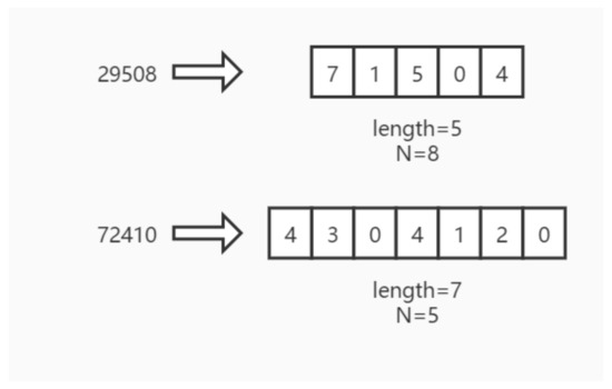
Figure 1.
The examples of N-ary individuals.
The corresponding encoding method called N-ary encoding and the number N is called the ary number. Basic binary encoded genetic algorithm [19], octal encoded genetic algorithm [20] and decimal encoded genetic algorithm [21] all belong to NGA.
In the single-objective optimization problem, high ary number encoded GA can search for the optimal area more quickly (faster convergence speed) at the beginning of the evolution; low ary number encoded GA can ensure the error between the result and the theoretical optimal solution is smaller in the late evolution [22]. Moreover, a high ary number encoded GA can better maintain the diversity of the population to jump out of the local optimal [23].
Based on NGA, DGA was proposed to combine the advantages of high ary number encoding and low ary number encoding. Since different ary number has different effects on different stages of evolution, the ary number can be selected for each generation to optimize the evolutionary effects. Therefore, the core idea of DGA is that ary number N should be reduced to 2 from a certain initial number with the increase of evolutionary generation according to a fixed function. The process of DGA for a maximum problem is shown in Algorithm 1.
| Algorithm 1: Process of DGA |
 |
In Algorithm 1, , and represent the genetic operators which are used to obtain a new population, is used to calculate the fitness function for the population, is used to find the optimal solution in the population.
Compared with the normal GA, the DGA re-encodes all the individuals in each generation. In addition, the ary number N for the next generation is calculated according to the change rule .
Because DGA combines the advantages of high ary number encoding and low ary number encoding, it has improvements on both convergence speed and optimization effect.
On this basis, many experiments have been carried out to examine the influence of the ary number’s function. Through the analysis and summary of the law between the change of the ary number and the change of the fitness function in DGA, we proposed an Adaptive Degressive Ary Number Encoded Genetic Algorithm (ADGA) [11]. Different from DGA, the change rule of the ary number in ADGA is adaptive. ADGA can give full play to the advantages of high-ary number encoding and low-ary number encoding in different evolutionary stages with a good universality.
In the single-objective optimization problem, degressive ary number encoding performs better than binary encoding. It can achieve better optimization results within fewer generations. Therefore, in order to improve the convergence speed of the multi-objective optimization algorithm, the degressive ary number encoding used in multi-objective problems is taken into account.
3.2. Model of Node Placement Optimization Problem
The node placement optimization problem is a high-dimensional multi-objective optimization problem. Through the optimization of WSN’s performance, the best moving position for each node is obtained. It can be simplified to a multi-objective optimization model with constraints.
The model of the node placement problem has been described in our latest paper [10] and the equations of the model are shown in Equations (2) and (3).
where are two matrices that represent the displacement of all the nodes’ coordinates, is the length of the monitoring area, is the width of the monitoring area, are the matrices of initial node coordinates, is a coefficient that restricts the movement of nodes, is the predicted rest energy set (including the moving energy consumption) for all nodes after operation for a period of time, represents the coverage of the WSN, represents the predicted rest energy of the node with the least energy in the WSN.
The traditional model of node placement optimization problem in WSN takes node coordinate as the solution. A node will move with the corresponding node number rather than move to the nearest position, resulting in a large distance. In this model, the coordinates of the node are replaced by the displacements of the node coordinates as the solution to the optimization problem. It can simplify the calculation of the moving distance, and help limit the moving distance of each node by restricting the search scope of the solution space.
Equation (3) shows that coverage and the minimum rest energy (includes node movement energy consumption) after a certain number of rounds are the two main optimization objectives. Since the minimum rest energy in all nodes can represent both the energy consumption and energy balance of the network, it can represent network lifetime.
4. Algorithm Design
4.1. Degressive Ary Number Encoded ADENSGA for Node Placement Problem
In previous studies [10], a directed evolved NSGA2, ADENSGA, was proposed to solve the node placement problem. In ADENSGA, the basic binary encoding is used. In this paper, we will further improve the encoding method of ADENSGA.
To improve the performance of the algorithm, degressive ary number encoding is considered to apply in ADENSGA. Thus, degressive ary number encoding should be extended to the multi-objective problems.
Encoding is a method which can transform the feasible solution of the problem from its solution space to the search space. Therefore, the implementation of degressive ary number encoding in multi-objective optimization problems is similar to that in single-objective optimization problems. The process of the degressive ary number encoded ADENSGA (D-ADENSGA) for the node placement optimization is shown in Algorithm 2.
| Algorithm 2: Process of D-ADENSGA |
 |
Some details in Algorithm 2 will be explained in the following.
- (1)
- calculates the number of overlapping at the location of the ith node according to the node density [10].
- (2)
- andand calculate the crossover probability and node movement range for each node, respectively, according to the node density at the location. The equations are shown in Equations (4) and (5).
- (3)
- , andand are the operators used in NSGA2 [19]. is a multiple-point crossover operator with the adaptive crossover probability .
- (4)
- (5)
- is used to calculate the objectives of the node placement optimization problem by Equation (3). represents the set of values of objectives for all solutions in the kth generation.
- (6)
- andis the elite strategy. selects the non-dominated solutions by the fast non-dominant sort. These two are also introduced in NSGA2 [19].
The change rule of ary number in D-ADENSGA can be expressed by a fixed equation. In other words, is determined in advance. However, it is uncertain whether degressive ary number encoding is effective in multi-objective optimization problems. In addition, the best change rule of ary number needs to be tested.
4.2. N-Ary Number Encoded ADENSGA for Node Placement Problem
Different ary number N may have different effects on the multi-objective problem than the single-objective problem. In order to apply degressive ary number encoding in a multi-objective problem, the optimization effect of multi-objective N-ary number encoding ADENSGA(N-ADENSGA) under different ary numbers N should first be tested.
The process of N-ADENSGA is exactly the same as D-ADENSGA in Algorithm 2, with during the whole process of evolution.
In this section, experiments are carried out on N-ADENSGA with different values of N.
In this experiment, set , the maximum iteration of the algorithm . The parameters used in the experiment are shown in Table 1.

Table 1.
Parameter Settings.
To comprehensively evaluate the optimization effect of the algorithms on the node placement problem, two auxiliary evaluation index and D is introduced [10]. represents the comprehensive performance of the algorithm. The larger the value of , the better the algorithm performance. D represents the total moving distance of all the nodes. The smaller the value of D is, the better the algorithm performance. The equations of and D are shown in Equations (7) and (8).
where , are the optimization objectives of the problem shown in Equation (3), is the moving distance of the ith node, n is the number of sensor nodes in the monitoring area.
The influences of ary number N for two different random node placements are shown in Figure 2 and Figure 3. Each figure is composed of (a), (b) and (c), respectively, corresponding to three evaluation indexes, average Coverage, average Rest Energy, and average .
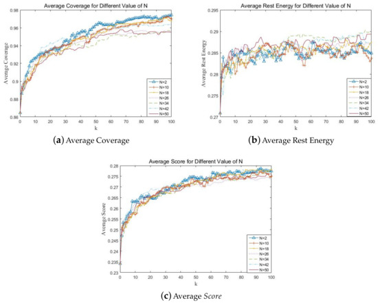
Figure 2.
The optimal results for different values of N of node placement 1.
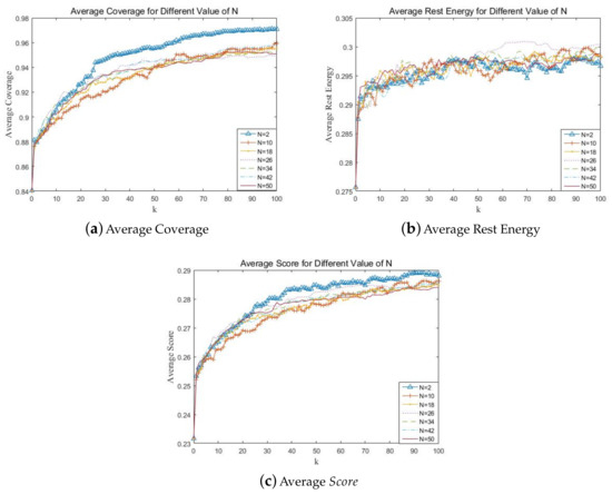
Figure 3.
The optimal results for different values of N of node placement 2.
Figure 2a and Figure 3a show that on the objective of coverage, low ary number encoding is significantly better than high ary number encoding in the final optimization effect, while high ary number encoding is more likely to optimize the objective faster in the initial stage of optimization (before 20 generations).
Figure 2b and Figure 3b show that on the objective of rest energy, high ary number encoding is better than low ary number encoding in the final optimization effect, and can optimize the objective faster in the initial stage of optimization.
Figure 2c and Figure 3c show that considering the two optimization objectives comprehensively, high ary number encoding can close to the optimization objectives faster in the initial stage of evolution, while low ary number encoding can get better optimization results in the middle and late stages of evolution.
Since the value ary number N can determine the size of the search space, it may affect the running time of the algorithm and the accuracy of the solution. In order to find out the relationship between the running time, D and N, the results for 10 random initial placements are calculated and shown in Table 2.
Table 2.
Running time for different values of N.
Table 2 shows that the running time and D have little relation with N. This is because that the running time of the algorithms mainly influenced by the predicting running of WSNs in . The influence of encoding length on running time can be negligible. Furthermore, the ary number N may slightly affect the precision of the solutions, but will not affect the total moving distance D of all the nodes.
4.3. Adaptive Degressive Ary Number Encoded ADENSGA for Node Placement Problem
Section 4.2 shows that in the multi-objective problem, the optimal ary number will change with evolution. Therefore, the multi-objective genetic algorithm with degressive ary number encoding is feasible to solve the problem of node placement in WSNs.
Through the experiment of N-ADENSGA, the rough degressive rules of ary number can be concluded:
- (1)
- To solve the problem that local early convergence leads to poor optimization results and maintain the population diversity in a high-dimensional problem, it is necessary to maintain a high ary number N for certain generations at the beginning of evolution;
- (2)
- In the process of N decreasing, the ary number N should decrease quickly first, then slowly and trend to 2 in the end;
- (3)
- The faster the is increased, the slower the ary number should be decreased.
Consequently, it can be supposed that the value of the next generation hexadecimal number can be determined according to the growth rate of .
Then an adaptive degressive rule of ary number can be proposed. The equation is shown in Equation (9).
where is the difference between the maximum and minimum values of the theoretical , is the initial average , is the initial ary number, is the ary number of the kth generation, is the generation when the ary number remains at , and is an estimation of the generation used when the ary number converges to 2. Among them, , , and are the default parameters.
The ary number of kth generation, , can be calculated by Equations (10) and (11).
where a is a parameter value to adjust the decreasing rate of ary number. In this paper, according to the experiment environment and experience, set , . The values of and will be discussed in the next section.
When the adaptive degressive ary number encoding is used in ADENSGA, a new improved algorithm called adaptive degressive ary number encoded directed evolved NSGA (AD-ADENSGA) is proposed. The process of AD-ADENSGA is shown in Figure 4.
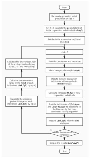
Figure 4.
The flow chart of AD-ADENSGA.
5. Parameter Analysis
The key to AD-ADENSGA is the adaptive calculation of . Equation (10) shows that the initial ary number and the highest ary number’s generation are the two main parameters. In this section, these two parameters will be tested and analyzed.
5.1. Parameter Analysis for Initial Ary Number
Initial ary number is used to set the encoded ary number of the initial population. The value of the initial ary number determines the rate of change of the ary number throughout the evolution process. If is too low, the algorithm will quickly degrade to a binary algorithm. If is too high, the algorithm is easy to fall into a locally optimal solution. Therefore, an appropriate initial ary number will help improve the optimization effect of the algorithm.
In this section, experiments are carried out on AD-ADENSGA with different values of .
In this experiment, set , , set 5 different values for . When , the algorithm is equal to the binary encoded ADENSGA. According to Section 4.3, set , . Other parameters used in the experiment are shown in Table 1.
The influences of initial ary number for a random node placement are shown in Figure 5. Each figure is composed of (a), (b), (c) and (d), respectively corresponding to four evaluation indexes, average Coverage, average Rest Energy, average and max .
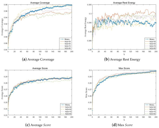
Figure 5.
The optimal results for different values of of node placement 3.
In order to observe the influence of on the optimization results more intuitively, the average ary number of five runs changing with the generation is shown in Figure 6.
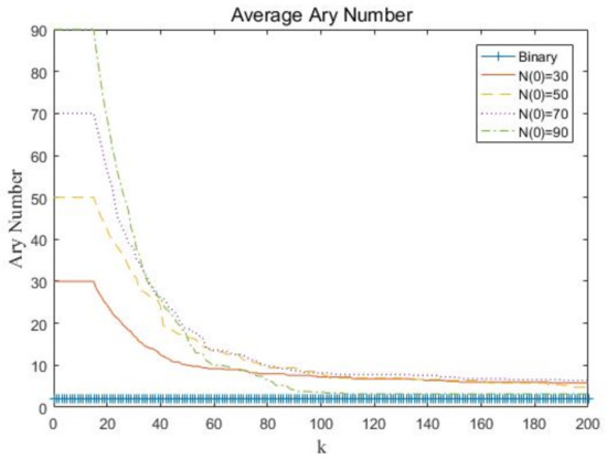
Figure 6.
The average ary number changing with the generation for different values of .
Figure 5a shows the influence of on the objective of coverage. When is too low, the optimization speed of coverage is poor. When is too high, the optimization speed is fast but the final results of coverage are poor. Figure 5b shows have little influence on the objective of rest energy. Figure 5c,d show that considering the two optimization objectives comprehensively, should be chosen in the range of 30–70.
Considering that is related to the encoding length, the value of may affect the running time. The average running time for different values of for 10 random initial placements are shown in Table 3.
Table 3.
Running time for different values of .
Table 3 shows that the running time has little relation with . This is because that the running time of the algorithms mainly influenced by the predicting running of WSNs in . Therefore, the algorithm with shorter convergence generation takes less time.
In this paper, considering the optimization objectives of coverage and rest energy, is chosen.
5.2. Parameter Analysis for the Highest Ary Number’s Generation
The highest ary number’s generation is used to set the generation of the initial ary number needed to remain. The value of the determines from which generation the ary number begins to decline adaptively. If is too low, the algorithm is easy to fall into a locally optimal solution. If is too high, the algorithm will need to spend much more time. Therefore, the selection of an appropriate highest ary number’s generation is very important.
In this section, experiments are carried out on AD-ADENSGA with different values of .
In this experiment, set , , set 7 different values for . According to Section 4.3, set , . Other parameters used in the experiment are shown in Table 1.
The influences of the highest ary number’s generation for a random node placement are shown in Figure 7. Each figure is composed of (a), (b), (c) and (d), respectively corresponding to four evaluation indexes, average Coverage, average Rest Energy, average and max .
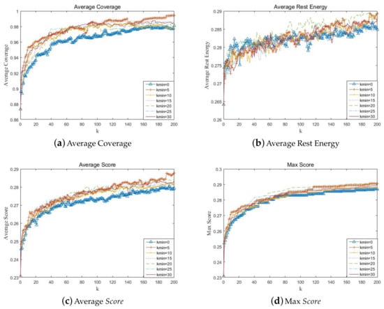
Figure 7.
The optimal results for different values of of node placement 4.
In order to observe the influence of on the optimization results more intuitively, the average ary number of five runs changing with the generation is shown in Figure 8.
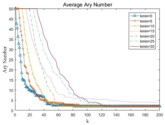
Figure 8.
The average ary number changing with the generation for different values of .
Figure 7a shows the influence of on the objective of coverage. When is too low, the optimization speed and final results of coverage are poor, the algorithm may fall into local optimum. Figure 7b shows has little influence on the objective of rest energy. Figure 7c,d show that considering the two optimization objectives comprehensively, should be chosen over 10.
In this paper, is chosen.
6. Results and Discussion
In this section, the AD-ADENSGA will be compared with ADENSGA with basic binary encoding (ADENSGA) [10] and decreasing ary number encoded ADENSGA with a fixed change rule of ary number (D-ADENSGA) mentioned in Section 4.1.
According to the rough degressive rules of ary number concluded in Section 4.3, a similar fitting function can be found as the degressive rule of D-ADENSGA, which is shown in Equation (12).
The experimental environment has been described in Section 4.2 and the parameters used in the experiment are shown in Table 1. In addition, set , , . According to the parameter experiments in Section 5, set , .
The curves of ary number changing with the generation are shown in Figure 9. The curves respectively represent the change of ary number for AD-ADENSGA in five runs, ADENSGA and D-ADENSGA.
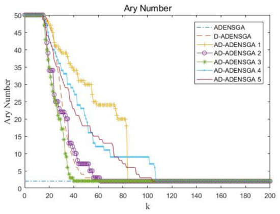
Figure 9.
The average ary number changing with the generation for node placement 5.
Figure 10 shows the results of ADENSGA, D-ADENSGA and AD-ADENSGA in each generation. Among them, Figure 10a shows the average Coverage curves, Figure 10b shows the average Rest Energy curves, Figure 10c shows the average curves and Figure 10d shows the max curves. The average Coverage curves, average Rest Energy curves and average curves respectively represent the average of the mean value of the first dominance level’s Coverage, Rest Energy and in five runs. The max curves represent the average of the maximum value of the first dominance level’s in five runs.
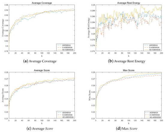
Figure 10.
The optimal results of ADENSGA, D-ADENSGA and AD-ADENSGA for node placement 5.
Figure 10a,b show that AD-ADENSGA and D-ADENSGA can achieve higher coverage in less time, while the optimization effect of AD-ADENSGA on energy consumption is better than D-ADENSGA and ADENSGA.
Figure 10c,d show that the optimization effects of both AD-ADENSGA and D-ADENSGA are better than ADENSGA.
To further analyze the optimization of these three algorithms, the results of the 200th generation () are shown in Table 4. Gn95 means the generation in which Average Coverage reaches 0.95 for the first time, where the optimal results are highlighted in bold.
Table 4.
Results for Node Placement 5.
Table 4 shows that the coverage and rest energy of D-ADENSGA and AD-ADENSGA are all much better than ADENSGA with less moving distance D. The optimization effect of AD-ADENSGA is better than D-ADENSGA and ADENSGA. In addition, AD-ADENSGA can obtain the required coverage faster than D-ADENSGA and ADENSGA.
In order to eliminate the contingency and ensure the optimization effect for different initial node placements, two other random initial node placements are tested in this paper.
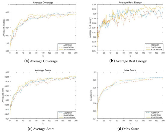
Figure 11.
The optimal results of ADENSGA, D-ADENSGA and AD-ADENSGA for node placement 6.
Table 5.
Results for Node Placement 6.
Figure 11a,b show that AD-ADENSGA can still achieve a certain coverage in less time, and it can also achieve a best optimization effect on energy consumption. However, the optimization effect and speed of D-ADENSGA are about the same as ADENSGA.
Figure 11c,d show that the optimization effect of AD-ADENSGA is better than D-ADENSGA and ADENSGA.
Table 5 shows that the coverage and the rest energy of AD-ADENSGA are much better than D-ADENSGA and ADENSGA. The optimization effect of D-ADENSGA is similar to ADENSGA, but with a longer moving distance D. In addition, AD-ADENSGA can obtain the required coverage faster than D-ADENSGA and ADENSGA.
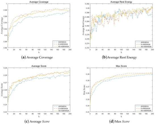
Figure 12.
The optimal results of ADENSGA, D-ADENSGA and AD-ADENSGA for node placement 7.
Table 6.
Results for Node Placement 7.
Figure 12a,b show that D-ADENSGA can achieve higher coverage in the least time, while AD-ADENSGA can achieve the best optimization effect on energy consumption. AD-ADENSGA can also achieve higher coverage in less time, but the speed is slower than D-ADENSGA.
Figure 12c,d show that the optimization effect of D-ADENSGA is better than AD-ADENSGA, and the optimization effect of AD-ADENSGA is better than ADENSGA.
Table 6 shows that the coverage and rest energy of both AD-ADENSGA and D-ADENSGA are much better than ADENSGA with less moving distance D. The optimization effect of D-ADENSGA is the best, but AD-ADENSGA can achieve a similar optimization effect with a shorter moving distance D. In addition, D-ADENSGA can obtain the required coverage faster than AD-ADENSGA and ADENSGA.
It can be concluded that both AD-ADENSGA and D-ADENSGA can achieve better optimization results than ADENSGA, among which, AD-ADENSGA has the best optimization effect, speed and stability. In other words, applying degressive encoding to a multi-objective optimization algorithm is beneficial to solve the node placement problem of WSN. Due to the fixed rule of degressive ary number encoding, D-ADENSGA can only achieve better optimization results in some initial node placements. The adaptive change rule of ary number proposed in this paper is feasible. It can improve the optimization performance and stability of the algorithm.
7. Conclusions
In this paper, degressive ary number encoding is applied to a multi-objective problem—node placement problem. By comparing and analyzing the optimization effect of N-ary number encoding for different ary number N, an adaptive degressive rule of ary number for a high dimensional multi-objective optimization problem is proposed. The appropriate parameters are determined through experiments. Based on ADENSGA, its encoding is improved to adaptive degressive ary number encoding, and AD-ADENSGA is obtained.
Experiments show that the improved algorithm has a significant improvement in convergence speed and the searching performance when solving the node placement problem. At the same time, the algorithm has good stability and universality.
Author Contributions
Conceptualization, Y.Z. and M.L.; methodology, Y.Z.; software, Y.Z.; validation, Y.Z.; formal analysis, Y.Z.; investigation, Y.Z.; writing—original draft preparation, Y.Z.; writing—review and editing, Y.Z. and M.L.; project administration, M.L.; funding acquisition, M.L. All authors have read and agreed to the published version of the manuscript.
Funding
The author(s) disclosed receipt of the following financial support for the research, authorship, and/or publication of this article: This work was supported by Fundamental Research Funds for the Central Universities, 222201917006.
Conflicts of Interest
The authors declare no conflict of interest.
Abbreviations
The following abbreviations are used in this manuscript:
| WSN | Wireless sensor network |
| GA | Genetic algorithm |
| NSGA2 | A Fast Non-dominated Sorted Genetic Algorithm |
References
- Pottie, G.; Kaiser, W. Wireless sensor networks. Commun. ACM 2000, 43, 51–58. [Google Scholar] [CrossRef]
- Bhuiyan, M.Z.A.; Wang, G.; Jie, W.; Cao, J.; Liu, X.; Tian, W. Dependable Structural Health Monitoring Using Wireless Sensor Networks. IEEE Trans. Dependable Secur. Comput. 2017, 14, 363–376. [Google Scholar] [CrossRef]
- Lv, A.; Li, C.; Xie, J.; Guo, W. Node Placement in WSN for Rail Track Monitoring System. J. Phys. Conf. Ser. 2018, 1060, 012044. [Google Scholar] [CrossRef]
- Wang, B. Coverage Problems in Sensor Networks: A Survey. ACM Comput. Surv. 2011, 43, 293–345. [Google Scholar] [CrossRef]
- Wang, R.; He, G.; Wu, X.; Wang, F.; Hu, Y. Research on suboptimal energy balance of non-uniform distributed nodes in WSN. J. Supercomput. 2018, 51–58. [Google Scholar] [CrossRef]
- Liu, X. A Deployment Strategy for Multiple Types of Requirements in Wireless Sensor Networks. IEEE Trans. Cybern. 2017, 45, 2364–2376. [Google Scholar] [CrossRef]
- Tsai, C. An effective WSN deployment algorithm via search economics. Comput. Netw. 2016, 101, 178–191. [Google Scholar] [CrossRef]
- Kapil, K.; An, B. Flower Pollination Optimization and RoI for Node Deployment in Wireless Sensor Networks. Inf. Commun. Technol. Intell. Syst. 2019, 106, 165–174. [Google Scholar]
- Ying, L.; Chin, K.W.; Yang, C.; He, T. Wireless sensor networks. IEEE Trans. Veh. Technol. 2019, 68, 6064–6073. [Google Scholar]
- Zhang, Y.; Liu, M. Adaptive Directed Evolved NSGA2 Based Node Placement Optimization for Wireless Sensor Networks. Wirel. Netw. 2020, 26, 3539–3552. [Google Scholar] [CrossRef]
- Zhang, Y.; Liu, M. An improved genetic algorithm encoded by adaptive degressive ary number. Soft Comput. 2018, 22, 6861–6875. [Google Scholar] [CrossRef]
- Long, T.; Sun, H.; Zhao, J. Research of mobile node deployment in WSN based on improved frog leaping algorithm. Comput. Eng. 2012, 38, 96–98. [Google Scholar]
- Gupta, G.P.; Jha, S. Biogeography-based optimization scheme for solving the coverage and connected node placement problem for wireless sensor networks. Wirel. Netw. 2018, 25, 3167–3177. [Google Scholar] [CrossRef]
- Abidin, H.Z.; Din, N.M. WSN sensor node placement approach using Territorial Predator Scent Marking Algorithm (TPSMA). In Proceedings of the IEEE Malaysia International Conference on Communications, Kuala Lumpur, Malaysia, 26–28 November 2013; pp. 13–17. [Google Scholar]
- Khalesian, M.; Delavar, M.R. Wireless sensors deployment optimization using a constrained Pareto-based multi-objective evolutionary approach. Eng. Appl. Artif. Intell. 2016, 53, 126–139. [Google Scholar] [CrossRef]
- Jourdan, D.B.; Weck, O.L. Multi-objective genetic algorithm for the automated planning of a wireless sensor network to monitor a critical facility. Proc. SPIE 2004, 5403, 1–11. [Google Scholar]
- Tripathi, A.; Gupta, P.; Trivedi, A.; Kala, R. Wireless Sensor Node Placement Using Hybrid Genetic Programming and Genetic Algorithms. Int. J. Intell. Inf. Technol. 2011, 7, 63–83. [Google Scholar] [CrossRef]
- Liu, M.; Qian, F. The research based on degressive ary number encoded genetic algorithm. Inf. Control 2004, 3, 614–617. [Google Scholar]
- Deb, K.; Pratap, A.; Agarwal, S.; Meyarivan, T. A fast and elitist multiobjective genetic algorithm: NSGA-II. IEEE Trans. Evol. Comput. 2002, 6, 182–197. [Google Scholar] [CrossRef]
- Li, D.; He, X. Comparison between optimization of function achieved by genetic algorithm with binary code and octal code. J. Zhejiang Univ. Technol. 2001, 29, 308–311. [Google Scholar]
- Ball, L.; Estel, L.; Cosmao, J.M.; Mouhab, N. A genetic algorithm with decimal coding for the estimation of kinetic and energetic parameters. Chemom. Intell. Lab. Syst. 2000, 50, 121–135. [Google Scholar]
- Yang, Y. Molecular Genetics. In Molecular Genetics; China Agriculture Press: Beijing, China, 2001. [Google Scholar]
- Qiu, X.; Tang, Y.; Meng, D.; Xu, Y. Multivalue coded genetic algorithm. J. Southwest Jiaotong Univ. 2003, 38, 227–230. [Google Scholar]
© 2020 by the authors. Licensee MDPI, Basel, Switzerland. This article is an open access article distributed under the terms and conditions of the Creative Commons Attribution (CC BY) license (http://creativecommons.org/licenses/by/4.0/).