Article

Application of the Reed-Solomon Algorithm as a Remote Sensing Data Fusion Tool for Land Use Studies

Faculty of Geography and Regional Studies, University of Warsaw, Krakowskie Przedm. 30, 00-927 Warsaw, Poland
Algorithms 2020, 13(8), 188; https://doi.org/10.3390/a13080188
Submission received: 22 June 2020 / Revised: 28 July 2020 / Accepted: 28 July 2020 / Published: 3 August 2020
(This article belongs to the Section Algorithms for Multidisciplinary Applications)

Abstract

:
The Reed-Solomon algorithm is well known in different fields of computer science. The novelty of this study lies in the different interpretation of the algorithm itself and its scope of application for remote sensing, especially at the preparatory stage, i.e., data fusion. A short review of the attempts to use different data fusion approaches in geospatial technologies explains the possible usage of the algorithm. The rationale behind its application for data fusion is to include all possible information from all acquired spectral bands, assuming that complete composite information in the form of one compound image will improve both the quality of visualization and some aspects of further quantitative and qualitative analyses. The concept arose from an empirical, heuristic combination of geographic information systems (GIS), map algebra, and two-dimensional cellular automata. The challenges are related to handling big quantitative data sets and the awareness that these numbers are in fact descriptors of a real-world multidimensional view. An empirical case study makes it easier to understand the operationalization of the Reed-Solomon algorithm for land use studies.

Graphical Abstract

1. Introduction

Remote sensing is the basic tool for obtaining a huge volume of digital information by sensing reflected electromagnetic radiation in a range of visible radiation, infrared, thermal infrared and microwaves, especially from satellite images. The spectral, spatial and temporal variation of electromagnetic energy coming from the scene contains the desired information [1]. More and more detailed information, inter alia, concerning land use—land cover (LU/LC)—is acquired, and several approaches, algorithms and computer applications have been developed, which are also aimed at the automatic classification of satellite images parallel to the development of both software tools and hardware devices. The main thread of this paper is the data fusion of all possible acquired information, which is used as a case study related to LU/LC identification, but primarily as the tool for data fusion. Further steps and application of further described procedures are left to be decided according the aims designated by researcher.
The growing importance of satellite images in environmental monitoring is related primarily to the recent rapid development of the Earth’s surface imaging systems [2]. Recent multispectral (MS) satellite images compound many spectral bands and resolution per spectral band that is above 8-bit resolution. Processing these images requires a lot of memory, time, and even a distributed processing approach. Several approaches to multispectral image segmentation allow various classes of LU/LC [3] to be detected, however the application of these methods is not limited to geospatial technologies and geodisciplines. It is further possible to classify some parts of images by defining the qualitative as well as quantitative characteristics of environmental elements and/or anthropogenic objects, using the combined visible and invisible spectral bands. Formerly used visual interpretation is time-consuming, even for the experienced researcher, and despite strictly defined procedures, it is rarely possible to obtain identical results, even when the action is repeated by the same person [2]. However, finally, a person will always need to evaluate the usefulness and correctness of the results of automatic classification using the set of information and communication tools (ICT) tools developed today.
The aim of this research is to verify the possible application of yet another spectral band data fusion approach using the Reed-Solomon algorithm (RS), which is well known in other fields of computer science. It should serve at the automation, preparatory stage of data acquisition, and is not intended to replace the well-defined procedures of the classification of satellite image content. We only aim to automate further steps of the detailed classification easier, e.g., LU/LC identification types. The novelty lies in the different interpretation of the algorithm itself and its scope of application. The empirical case study and the short review of the attempts to use different data fusion approaches in geospatial technologies explains the possible use of the RS algorithm. Moreover, the whole procedure is not in its final form of a complete computer application yet. Some steps are automated using scripting languages, but open source and commercial computer applications have been used at the stages of visualization and interpretation.
The rationale behind the application of the RS algorithm for image data fusion includes all possible information from all the acquired spectral bands, assuming that complete composite information in the form of one compound image will improve both the quality of visualization and some aspects of quantitative analyses. Passive optical hyperspectral, multispectral and panchromatic imaging technologies, as well as topographic information, acquired active sensors, light detection and ranging (LiDAR), and synthetic aperture radar (SAR) may be sources of image data fusion, making interpretability easier due to the diversification of information. One-modality of observations may be difficult to interpret [4]. A statistical sample of research projects concerning LU/LC revealed that data fusion provided results with higher accuracy than either of the datasets individually [5].

1.1. Radiometric and Spectral Resolution

Remote-sensors record the electromagnetic properties of land surface and the energy reflected (optical sensors), emitted (thermal infrared or passive microwave sensors) or scattered (active radar sensors), and hence provide a variety of information on land properties [5]. Currently, satellite images are simultaneously recorded in several or more electromagnetic radiation ranges, i.e., spectral bands: multispectral (MS) or hyperspectral (HS). Radiometric resolution, i.e., the precision with which the sensor can distinguish the variability of the electromagnetic radiation reaching it, is recorded in bits (eight and above). In other words, the number of digital levels used to express the data collected by the sensor. An 8-bit recording value of the variability of the reflected one-spectral-band varied between 0 and 255, thus representing greyscale. Therefore, the recorded information (of pixels in the acquired image) contains a set of different values (integers) with respect to the number of spectral bands. The values differ depending on the observed object (feature and place), condition and wavelength. Sometimes, features are indistinguishable in a certain spectral band, while they are quite different in another [3]. Spectral resolution is the number of spectral bands in which the sensor can collect reflected radiance; hyperspectral sensors collect hundreds of bands, moderate ones—in tens of bands, and low—three bands. These two definitions concerning radiometric and spectral resolution define two important parameters for the proposed algorithm, which is described further as values of pixels and the number of spectral bands. Other characteristics of a satellite image concerning spatial and temporal resolution are not currently taken into account in this paper due to the omission of these dimensions.
All the procedures described below (for an end user) are assumed to operate on the same radiometric resolution (a condition which is fulfilled e.g., for Landsat ETM+), regardless of the number of spectral bands. For example, the EnMAP project acquires 14-bit resolution images. However, the resulting images are corrected to obtain radiometrically-calibrated radiance data. EnMAP final products characterize the strictly defined quality of images, which are different for different processing levels (level 0–8 bits, time-tagged instrument raw data with auxiliary internal information, level 1B, radiometrically corrected, spectrally and geometrically-characterized radiance, etc.) [6].

1.2. Image Data Fusion

Data fusion concerns the analysis of several datasets, which can interact with themselves and inform each other [4]. The problem of image data fusion is general and is not only related to remote sensing. The fused image “retains all the complementary and redundant information of the input images” [7]. The requirements of the fused image have been defined as retaining complementary and significant information regarding the input images, no presence (or minimization) of artefacts, i.e., appearance of synthetic features not present in real world, and last but not least, should not reduce the quality of view, e.g., noise or fault registration, or the elimination of inconsistencies [1,7,8]. The same requirements concern the remote sensing images, as well as the growing significance of the analysis of medical images, using relatively new approaches like, e.g., sparse representation and guided filtering. Similar approaches were aimed at the same targets, but in quite different fields [7,9,10]. There are numerous motivations for image data fusion: obtaining systemic global view of fused image, ease of exploratory research aimed improving decision-making, obtaining the answer to specific questions concerning distinctive modal elements (also in time) and extracting knowledge from image data for various purposes. Despite the numerous research papers on the topic, some researchers confirm the opinion that image data fusion is in its preliminary stages [4]. Challenges arise because fusion images concern the visualization of very complex phenomena, which are often dependent on a large number of synergistic features, either biological, environmental, sociological, psychological or urban systems (just to name a few). Such a wide spectrum of phenomena generates, in turn, a diversity of research problems. Visualization during the image fusion process is often based on heterogeneous input images and datasets. [4,11,12,13,14,15]
Earth observation (EO) initiatives play a key role in long-term remote-sensing application domains, such as LU/LC mapping, environmental monitoring, and natural resources, as well as in on-demand situations (e.g., crises), when EO data need to be streamed through time-critical workflows to deliver reliable and effective information [16]. Mapping the complexity of land use/land cover is a challenge, especially in regards to monitoring and managing the environmental and societal impacts of land use. Data fusion providing synergistic information appears to be a promising approach [5]. The challenging and ubiquitous remote-sensing image classifications of land use and land cover are mandatory in multi-temporal studies and are useful input for other research areas. The important challenges to the approach are related to the complex statistical characteristics of images involving high computational problems [17].
The application of classic methods of satellite image content detection of LU/LC is well-known and has a defined procedure using unsupervised or supervised classification or both. There is also the pre-preprocessing step that serves as an integral segment that stands in between data acquisition and analysis steps. Data fusion serves as a cohesive component and routine procedure in rapid information production [18]. It is also a general and recognized research problem involving quantitative and qualitative aspects [18,19,20,21,22,23,24]. The choice of algorithms used in data fusion depends on the scene and purpose of application. A deep insight and review of the possible approaches and algorithms (both open source as well as proprietary) can lead one to find rich literature on the subject. Specialists pointed out that the high spectral resolution is needed in order to classify complex land-use and land-cover types and fusing panchromatic (PAN) and MS images with complementary characteristics can provide a better visualization of the observed area [18,19,25,26,27,28]. There are several different fusion algorithms. The most known and used are: Intensity Hue Saturation (IHS), Modified IHS, principal component analysis (PCA), Pansharp, wavelet-based techniques (Wavelet), Local Mean Matching (LMM), Local Mean and Variance Matching (LMVM), Brovey transform (BT) and Multiplicative [23,29]. There are well-known constraints and advantages to the use of them. All of them transform input images, however only few preserve the spectral fidelity of the input dataset [23]. There are also so-called hybrid approaches; researches combine two or more fusion algorithms. Some of them combine different methods, e.g., General Intensity Hue Saturation (GIHS) with genetic algorithm (GIHS-GA), IHS with the Fast Fourier transform (FFT, called Ehlers fusion) [29,30]. Some proprietary and patented approaches offer users the adaptation of the fuse methods aimed at spectral integrity, high spatial detail in an intelligent manner depending on the context and target of the image fusion process [29,31], as well as the use of artificial intelligence (AI)
Multi-source image data fusion is perceived as the main tool aimed optimization and information extraction from remote-sensing data, and integrates more than three spectral bands [29,30,32]. Several software packages (e.g., ENVI, PCI, ERDAS, etc.) included fusion algorithms as available standard routine functions [29]. However, remote-sensing image fusion is possible using different sources, e.g., satellite and airborne, as well as hyperspectral and LiDAR (Light Detection and Ranging) images [29,33,34].
The diversity of sources forced new tools (algorithms) to be applied due to new challenges concerning the details of images as well as their parameters, often enumerated as the prioritized sequence of tasks. The prime challenge (mentioned above) concerned the appropriate methods of synthesis of all those multi-source images and/or data sets. The challenge of multiplying spectral bands is also related to changes in the range of the spectral band of new-generation sensors, which in turn affects the quality of the fused image. Other challenges (the threads not touched thereafter) concerned: geometric accuracy, different non-orthogonal angles of acquired observation images, and geometric and radiometric requirements for fused imagery [19,29].
There are different approaches to data: signal, pixel, feature and decision level fusion. At the signal level, fusion is aimed at creating a new, better quality signal. Compound images create, at the pixel level (fusion created on a pixel-by-pixel basis), an ease to image processing, especially in remote-sensing, medical diagnosis, surveillance and photography applications [35,36,37,38,39]. At the feature level, fusion highlights some overall parameters like pixel intensities, edges or textures. At the decision level, the fusion multiple methods are applied to elaborate on decision rules and are aimed at leveraging the interpretation of the image, which is usually used in artificial intelligence (AI) techniques [1,40,41]. Some researchers also point to the subpixel fusion level, which involves different spatial scales and uses appropriate transformation [41].
Pixel-level image fusion is perceived as the approach that directly combines the original information in the source images, and is aimed at synthesizing a more informative fused image for visual perception as well as computer processing. The main factors leveraging this approach are: (1) the need for combining images from different sensors and camera settings, (2) the development of signal processing and analysis theory, and (3) the growing amount and diversity of acquired images in different fields of applications. Pixel-level image data fusion now a set of tools that can be categorized into four groups: multi-scale decomposition methods (multiresolution analysis), sparse-representation-based methods (component substitution), the methods performing fusion directly to the image pixels or the group of pixels (model-based) and hybrid, mixed methods that combine two or more of the tools mentioned above [1,39].
There are numerous, mature approaches of multi-scale decomposition methods: pyramid and wavelet transformation [39,42], discrete wavelet transformation [39,43], stationary wavelet decomposition [44,45]. Other newer methods in this group are dual-tree complex wavelet [46], curve-let [47], contour-let [48,49], and shear-let [50,51]. The overwhelming majority of these methods use a dedicated filter applying either mathematical (e.g., directional or bilateral filters) or statistical kernels (e.g., weighted least squares filters). The main challenge concerns the lower quality of the resulting fused image (less satisfactory), as well as the decreasing computer efficiency [39].
Sparse representation-based methods simulate a mechanism of human seeing, assuming that only a few characteristics represent the acquired original images enough to be described. The outline of the method involves the creation of a dedicated coded procedure as well as a dedicated dictionary. The outcome is fused sparse coefficients, which, together with the dictionary, reveal the fused image [52,53].
There is also a group of methods that operate directly on pixels. The outcome pixel in the fused image may be the weighted average of the corresponding pixels of the input images. The weights may be evaluated using different algorithms: supported vector machine (SVM) or neural networks using also appropriate image segmentation, e.g., edge preserving or majority filters [54,55]. Other methods use PCA and are aimed at evaluating weights. However, these approaches are assessed as quite limited in relation to data fusion performance. Additionally, there are other procedures used, based on color space as well as dimension reduction [39]. Intensity, hue and saturation (IHS) transform are extensively used [56,57] for the panchromatic sharpening (pansharpening) problem. This method uses mathematical transformation that converts Red, Green, and Blue (RGB) values into a model of IHS, which represents human color perception, but may produce color distortions in the fused image [39]. There is also a patented method for enhancing the spatial resolution of multispectral imagery using pansharpening (Gram-Schmidt transformation [58]).
The last category of approaches uses combinations of two or more of the above-mentioned methods. The rationale behind such a procedure is based on the intention to link special advantages of certain methods. A detailed description of the advantages and shortcomings of such transformations is beyond the main thread of this paper and is presented elsewhere in numerous papers [39,59,60,61,62,63,64]
All of the above-mentioned methods touch the main problem of decreasing visual distortions when fusing multi-spectral, hyperspectral, and panchromatic images at the pixel level. Pixel-level image data fusion is directed at one of the most important techniques to integrate information from multiple sources, allowing for a comprehensive analysis of the captured scene [39].
The approach described below is related closely to (Geospatial) Object Based Image Analysis (OBIA or GEOBIA), which is directed as the paradigm of new methodology to classify or map VHR (Very High Resolution) images into meaningful objects, i.e., the grouping of relatively local homogenous pixels. The steps of the procedure involve a sequence of image segmentation, object classification and final detection results. The input image is segmented into homogenous regions (objects) that represent a group of pixels, and then the classification procedure is applied. These functions are implemented into almost every geographical information system (GIS) and has been widely used for land cover and land use mapping and tracing changes [65,66,67,68,69]. Next, there are different methods using several algorithms that can be applied, which are aimed at classifying objects as detection results.
The review of the classification methods is beyond the scope of this study, however interesting approaches related to data fusion are also considered in the context of the accuracy of classification results [70]. However, the multi-resolution segmentation (MRS) algorithm (implemented in eCognition®, Trimble Geospatial Imaging software) also needs to be mentioned. However, several problems remain and concern the lack of full automation and the need for expert knowledge to define the classification rules [65].
Remote sensing images need approaches to reduce the high dimensionality of data. There are several methods and algorithms used to do this. Some of them (mentioned above) are applied at the preparatory stage, i.e., the data fusion step. Other methods, related to image classification, operate on raw data or omit this first step. The classical PCA method is nowadays replaced by other non-linear dimensionality reduction methods, and manifold and dictionary learning algorithms, especially deep learning using convolutional neural network trained with an unsupervised algorithm promoting feature sparsity [17].

2. Methods and Materials

2.1. Reed-Solomon Codes (RS Algorithm)

2.1.1. Experience and Reinvention of the Algorithm

Our approach originated from studies of LU/LC changes using final products of the European research project CORINE (Coordination of Information on the Environment) Land Cover (CLC), maps and data sets, as well as attempts to use cellular automata applications and further research projects [71,72,73,74,75,76]. Applications, aimed at predicting LU/LC changes, as well as the valorization of landscapes, did not used remote-sensing images as the input datasets at all. The final formula of the algorithm was expressed in mathematical form in 2012 [74]. This concept arose from the empirical, heuristic combination of geographic information systems (GIS) map algebra and two-dimensional cellular automata. Later, awareness of the robust form of algorithm (described below) was the reason for looking for its application in different fields. It turned out that the mathematical formula was identical to the known formula of a wide range of used Reed-Solomon codes (RS algorithm).

2.1.2. Deeper Insight into the Reed-Solomon Algorithm

Reed-Solomon codes are a group of error-correcting codes that were introduced by Irving S. Reed and Gustave Solomon [77]. They have many applications, the most prominent of which include consumer technologies such as CDs, DVDs, Blu-ray Discs, QR Codes, data transmission technologies, such as DSL and WiMAX, broadcast systems, such as DVB and ATSC, and storage systems, such as RAID 6. They are also used in satellite communication [78]. The vital and robust method of RS codes are applied in cryptography, steganography and against the salt and pepper noise of medical images [79,80,81].
The original Reed-Solomon algorithm is a simple encoding procedure of a message as a sequence of coefficients in the formula (Equation (1)) [78]:
p x ( a ) = i = 1 k x i a i 1 .
Assumption: a, k, and x are positive integers and x ∈ <0,1,…, a>.
Without describing in depth the mathematical proof and only observing the empirical values of the above formula application, it was found that knowledge of a and k parameters meant the obtained value of px(a) could be decoded into the exact set of input of positive integer values x using only the recursive procedure of Euclidean divisions and recording the remainders. This is the practical application of the Chinese remainder theorem.
Value px(a) can be a huge positive integer, which can encode integer values (also representing nominal values). The method is universal, and the only limit is computer resources. Value px(a) is reversible. It is possible to reconstruct (recalculate) the original input of different sets of integers representing, for example, a nominal or interval scale only on the basis of certain parameters k and a, assuming that these input values are positive integers and value x ∈ <0,1,…, a >.

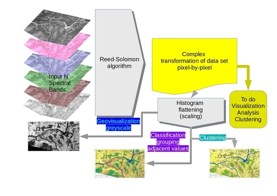
2.1.3. Application of the Reed-Solomon Algorithm for Remote Sensing Data Fusion

The procedure assumes that parameter a corresponds to the maximal value of radiometric resolution. It will be value a = 255 if the greyscale is coded; then the values of x can range from zero to 255. Again, parameter k corresponds to spectral resolution, i.e., the number of spectral bands in which the sensor can collect reflected radiance, i.e., for a Landsat ETM+ satellite image there are nine bands, the maximum value of k = 9 and k ∈ <1, 2, 3, 4, 5, 6, 7, 8, 9> (Algorithm 1).
Algorithm 1 Reed-Solomon Pixel-Level Algorithm for Remote Sensing Data Fusion
1: input a = 256//integer, number of values of radiometric resolution
2: input k = 9 //integer, number of spectral bands (raster layers)
3: input x (row, col, i) //integer, current pixel value in a stack of raster layers for certain row and column
4: output PX //integer, outcome pixel final value
5: intermediate output ppx[k] //set of integers
6: PX = 0
7: for i in range (k)
8:      ppx(i) = x (row, col, i) //get current pixels value in a stack of raster layers for certain row and column
9: for i in range (k)
10:    PX = PX + ppx(i)*(a**(i − 1))
11: print PX

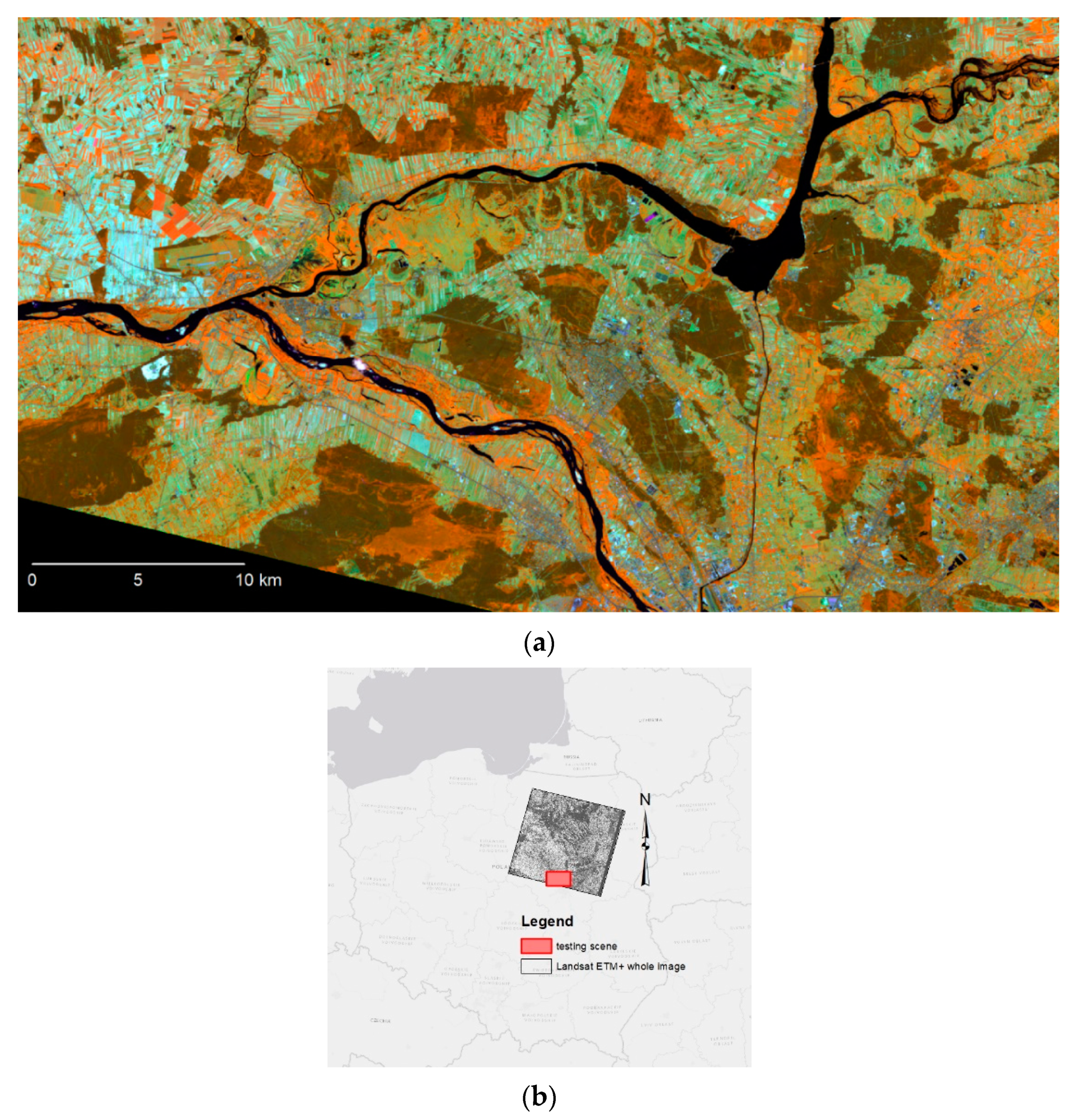
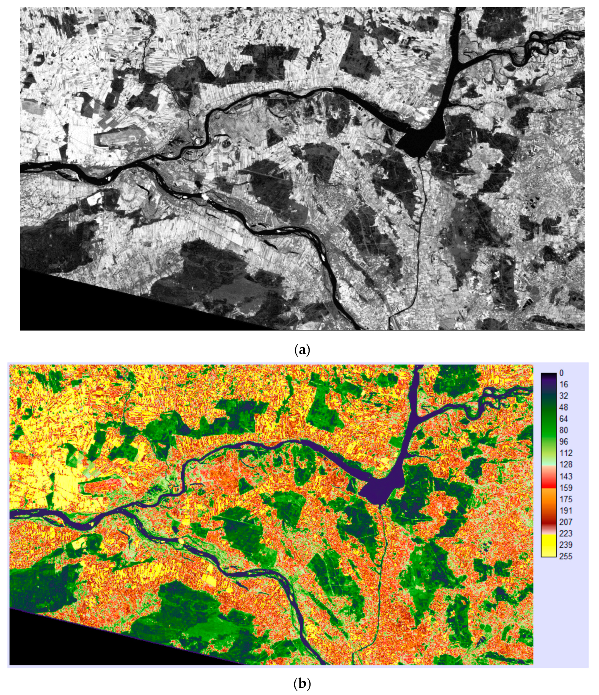
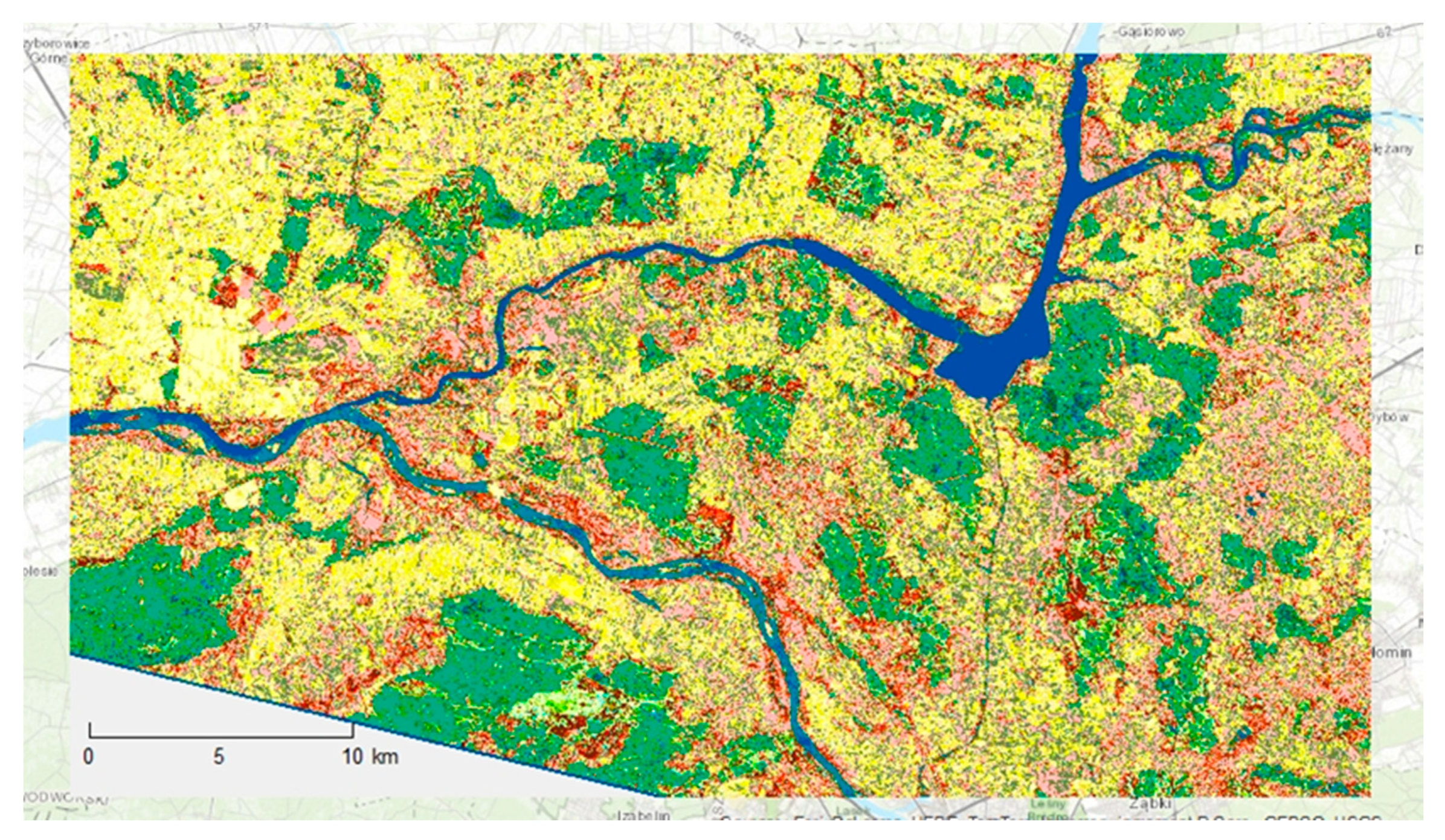
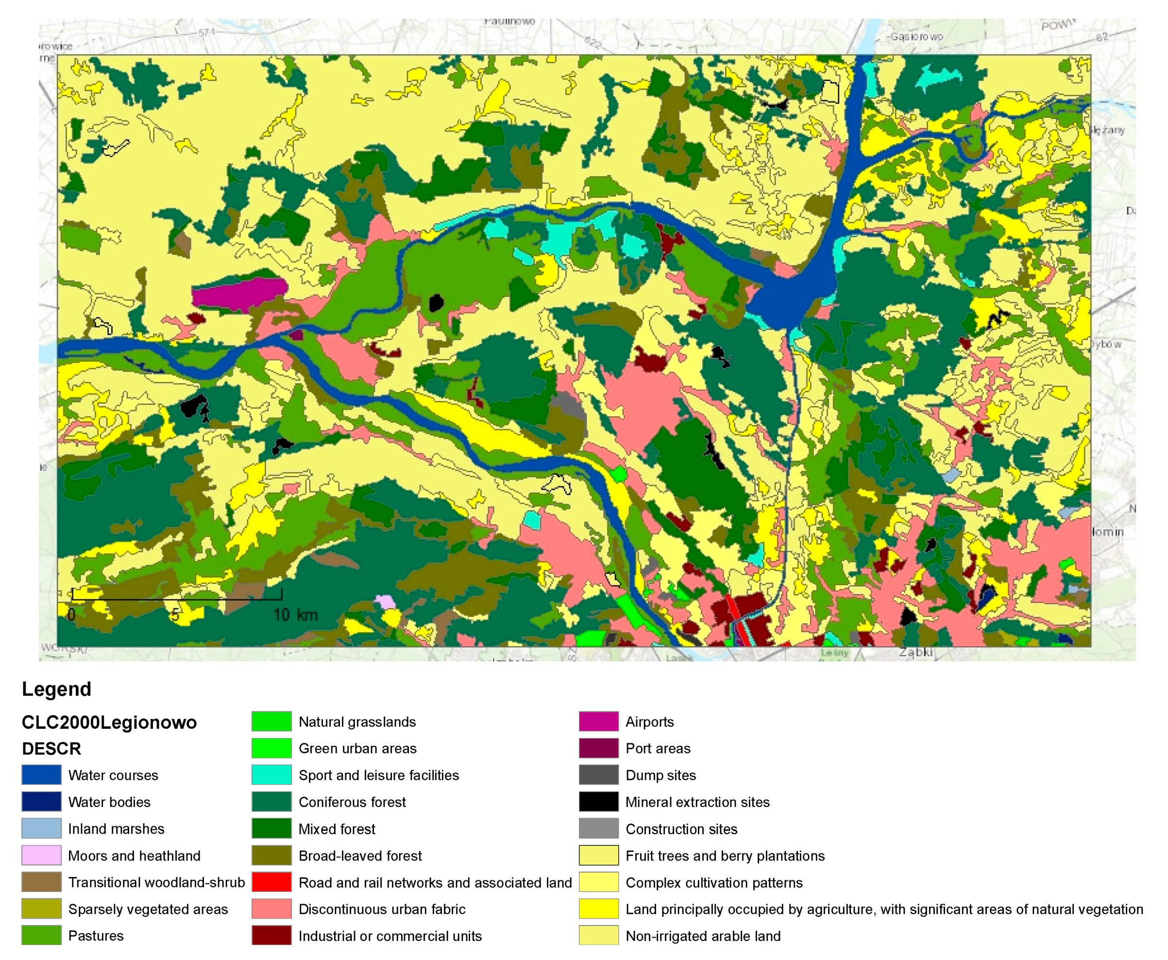
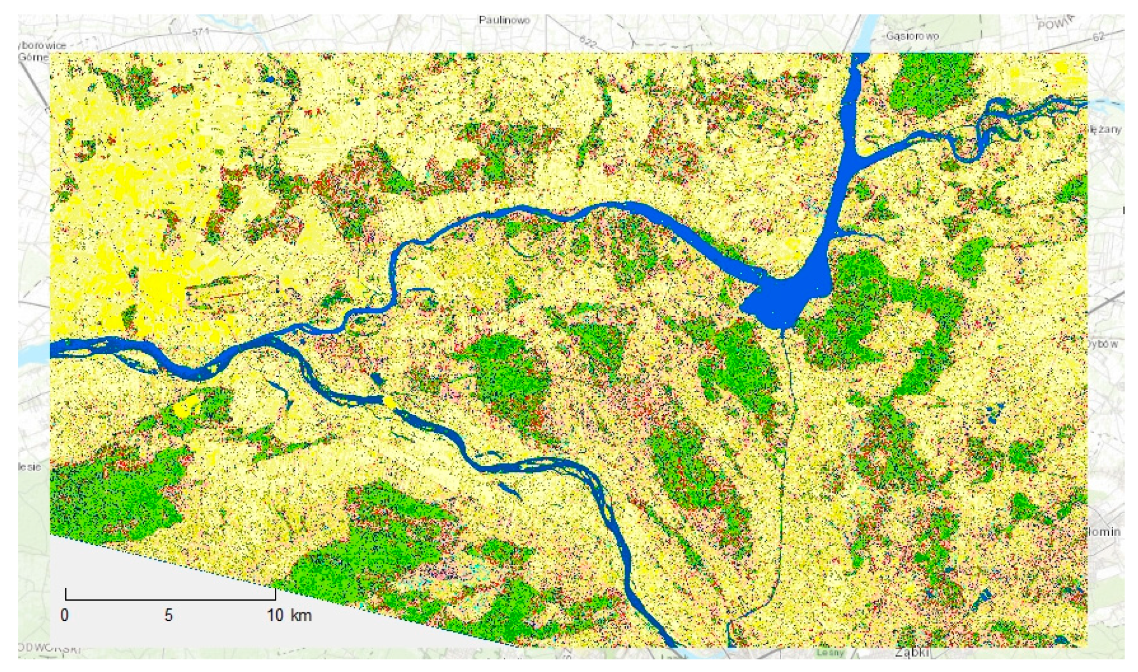
2.2. Empirical Verification Case Study of Neighborhood of Legionowo Area
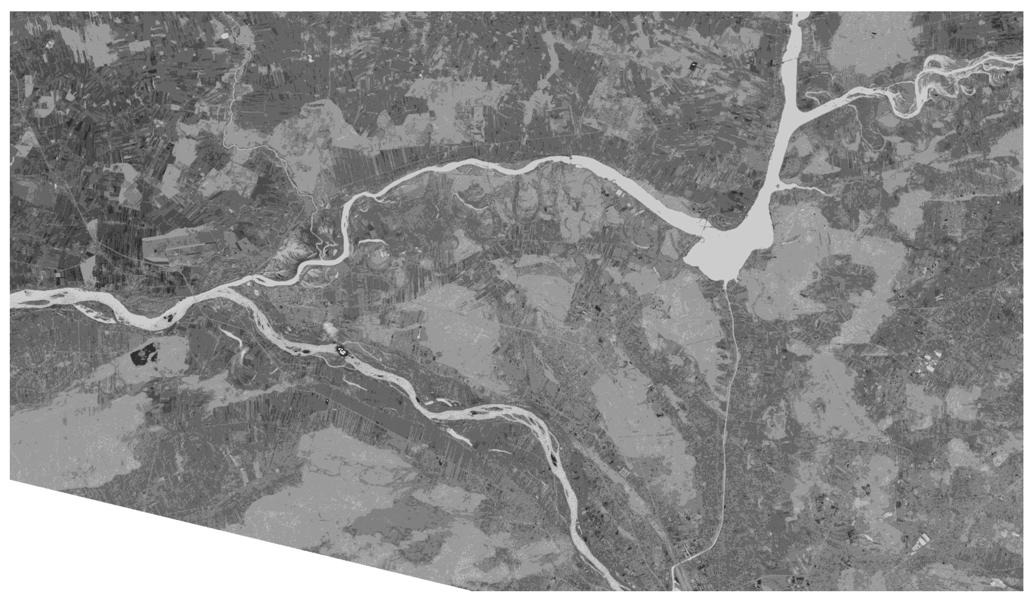
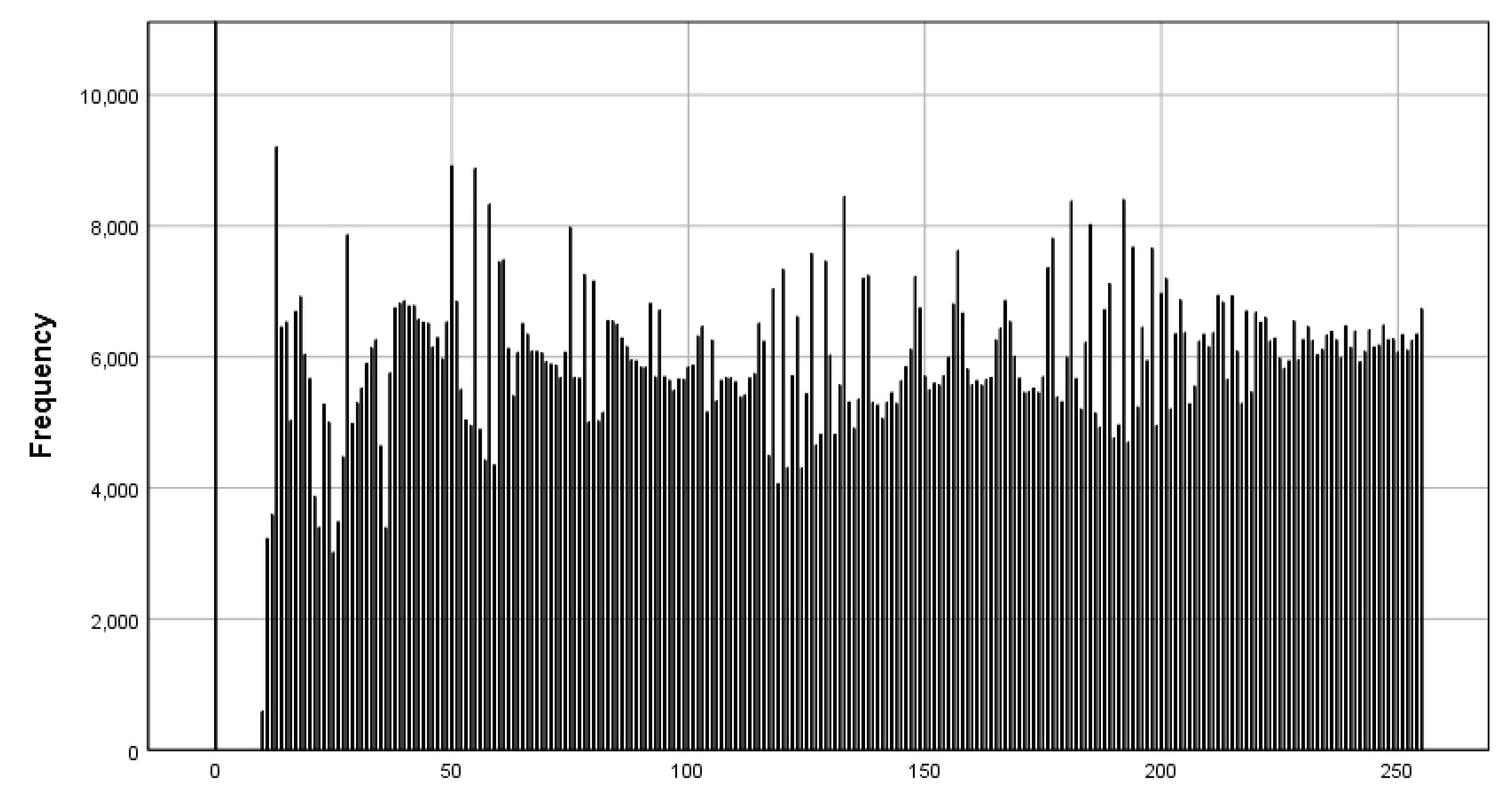
The testing scene is an area covering 1326.2 sq.km, located in the central part of Poland on the Mazovian Lowland near Warsaw. In its center, between the Vistula and Narew rivers, is the city of Legionowo (54 K inhabitants in 2019). There are coniferous and deciduous forests, agricultural areas, and meadows and buildings, and this is mainly a dispersed built-up area. Agricultural areas are characterized by a high degree of fragmentation. Small fields, often below one ha, are adjacent to the grasslands. On the Narew River there is an artificial reservoir, Zalew Zegrzyński, with an area of over 30 sq.km [2]. The satellite image of the polygon is shown in the Figure 1.
The testing scene was chosen because the area had been studied and classified in detail twice before. The first was a visual interpretation of the images taken by the Landsat TM satellite, according to the uniform European CLC legend based on a study carried at the Institute of Geodesy and Cartography (2000, shared by the Polish Main Inspectorate of Environmental Protection) [82]. Second, a similar (but smaller) area was also the topic of a research project aimed at object-oriented classification to obtain information on land cover and land use [2] at the same time. The scene and the same year were intentionally selected and the same satellite image was used to check the usefulness of the procedure for the preparation of input data fusion. The map tile also covers an area not covered by the image in the south–west (left corner of image).
The source was part of Landsat ETM+ scene [83]. The basic parameters of the image are available as a metadata file separately. The only correction concerned spatial resolution of panchromatic band No 9 (generalization of spatial resolution from 15 to 30 m). There were nine spectral bands. They were numbered 1 to 9 (as the k parameter for the RS algorithm). The spectral resolution was left intact.

3. Results

Calculation of the RS algorithm was not quite routine for all of the aforementioned spectral bands. There were computer software applications that were not able to handle the huge integer number calculations. The results of RS algorithm geocomputation in the form of a report are presented in Table 1. The algorithm was computed as an expression of the raster calculator (using the Golden Software Surfer mathematical function).

Visualizations

Visualization of the final results of geocomputation in the form of an image is possible; however, it is critical, due to the automatic clipping of raster, to have huge integer values by most open source and commercial computer GIS applications to different maximal values.
The result is one map containing all the information from the nine spectral bands. It is reversible, which means that information about any spectral band can be extracted from it. This is possible because of the simple scalar multiplication and summation of stacked pixel values from all spectral bands using the vector (2560, 2561, 2562, …, 2568). The reverse procedure involves recursive divisions and distribution of appropriate remainders using the above values.
No GIS software (available at this moment and known to the author) was able to display the full histogram of the image (most clipped the maximal values). Visualization of the resulting image containing information from all the spectral bands was possible using the export to a 24-bit depth geotiff file (presented in Figure 2).
That is why the original resulting image was rescaled into the range <0, 255>, rounding off the values to the nearest lower positive integer (again using the raster calculator). The flattened histogram, i.e., the greyscale values, are presented in Figure 3 and spatially visualized in Figure 4.
The resulting rescaled image can be visualized as a single band, greyscale image (in Figure 4a). This is an artificial procedure that develops a false image, it is however sufficient, at present, in order to illustrate the usefulness of all the aforementioned steps. This visualization involves all the data from the nine bands of the Landsat ETM+ original satellite image. However, due to rounding and rescaling, the original input values of the band components cannot be reconstructed (excerpted from the transformed image). It is only possible to obtain these data from the original outcome of the RS algorithm application. The transformed image seems to be very sharp; the details are distinguishable, and are comparable to other results of the above-mentioned algorithms and methods of the data fusion. The same image displayed using pseudo-color technique reveals some more details (Figure 4b).

4. Remarks

The properties of the above-described procedure makes it possible to segment the resulting image automatically, using only initial (unsupervised) classification of fused image, displaying each level of the greyscale as a different color (pseudo-color technique). Detailed identification of land use classes is the next step and needs use of dedicated (supervised or unsupervised) procedures and algorithms (beyond of the scope and aim of this research). The next step involved only the use of a clustering method—grouping the adjacent (close) values of the image (levels of greyscale, omitting their number, i.e., count)—and it was automatically displayed into the 256 clusters (Figure 4b). This clustering procedure was recursively repeated using a manual trial-and-error method of classification that was aimed at adjusting the final classification until a (subjectively) satisfactory result was obtained. The procedure started with the grouping of the ten lowest values, after which water bodies and courses appeared. The reference map was a sheet of an original CLC 2000 map of the same area. No especially dedicated classification procedures were applied; only the grouping of the adjacent values of the flattened image and searching for correspondence to the reference CLC generalized map colors as well as the World Topographic (base) map. Visualization of a single band, pseudo color and manually clustered (of adjacent values) image of the transformed and rescaled outcome of the RS algorithm application on the original Landsat ETM+ satellite image, involving information from all nine spectral band components, is presented in Figure 5. The colors are similar to the legend of the CLC 2000 map (Figure 6). The resulting image is displayed as a layer on top of the topographic map.
Simultaneously, the unsupervised k-means procedure for clustering (using SAGA GIS) resulted in another map (Figure 7) using a legend color palette similar to that applied during manual identification of the 24 LU/LC classes referenced to the above-mentioned maps (again checking only that they matched visually).
The amount of time spent to generate the results of the RS algorithm computation for the whole Landsat ETM+ image (for nine spectral bands, 7451 rows and 8121 columns) is not available due to the overflow memory error. For testing the scene (939 rows x 1641 columns), the application of raster calculator lasted a few minutes. A computer with an Intel® Core™ i7-2760QM CPU @ 2.40GHz processor with 16GB of RAM was used. Rescaling the resulting image into the greyscale took 1–2 min to test scene. The duration of the initial, unsupervised segmentation of the rescaled resulting image was immediate, but the classification using k-mean clustering for 24 classes lasted over an hour (Figure 7).

5. Discussion

All of the operations described above deliberately omitted flexible, complex procedures using sophisticated algorithms of unsupervised or supervised LU/LC classifications. The aim was only to check whether the application of the RS algorithm outcomes was reasonable, and the aim was not complete because precise classification of land use types was not finished. The RS algorithm was applied as a data fusion tool, and further arithmetic operations concerned the digitally represented reflected electromagnetic radiation. However, the resulting (synthetic) image represented the nominal scaling, i.e., each small or huge integer value of any pixel in the resulting image corresponded to a unique combination of compound values of the set of certain spectral bands. This is a mutually unequivocal function. Any further transformation of the resulting image may destroy this function. This means that grouping (e.g., coloring) and/or clustering the pixels while retaining the original input values of pixels is safe. Further, the RS algorithm created data fusion that layered (stacking) the sequence of input values as groups differentiated by an order of magnitude of numbers.
The initial automatic classification of resulting fused image was the final step of data fusion procedure using the RS algorithm. It seems that the main thread and aim of the research had been obtained. However, there are further steps related to precise identification of land use types, which use well-known generalization and supervised or unsupervised methods of classification. The idea of using a similar approach, in the form of another use of RS algorithm, was signalized in former studies [75]. The only condition was the accurate and detailed development of the image data fusion method using the RS algorithm prior to that. These next steps of classification appeared as another thread and the subject of separate studies (beyond the scope and aims of this paper).
Sample application of the data fusion resulting image concerning LU/LC classification is only one thread of the RS algorithm application, but shows the possible simple ways of visualization and analysis in further steps. The challenge is to find a way to display the outcome, synthetic image as well as its histogram. No GIS software tools available (available and known to the author) can do this without additional operations, which unfortunately destroy this precision and make it impossible to recalculate (reconstruct or extract) the original spectral band inputs.
Another aspect is related to statistical analysis of the resulting image. Due to possible treatment of the resulting image as a set of qualitative features (represented by the sequences of integers), some non-parametric approaches may be applied in further steps. These would be preferably median or mode, and quantiles, because these parameters can be reconstructed (recalculated) and the input combination of the values of given spectral bands can be shown.
An example of a reverse procedure for obtaining the original input of spectral bands from the (random) pixel value of the resulting image is presented in Table 2. These are recursive steps of modulo division using parameter α for a sequence of obtained quotients.
The RS algorithm may be theoretically applied to any positive integers, i.e., there may be any number of spectral bands and any number of levels of registered electromagnetic radiation in the above-described problem of LU/LC classification. The RS algorithm can evaluate them, but the only limits are related to hardware and software resources. The only requirement is constant input parameters α and k. The hidden assumption is a strictly defined ascending sequence of calculation, which must be reproduced in the reverse procedure (Algorithm 2).
Algorithm 2 Reed-Solomon pixel-level reverse algorithm for remote sensing data fusion
1: input a = 256 //integer, maximal value of radiometric resolution, divisor
2: input k = 9 //integer, number of spectral bands (raster layers)
3: input PX //integer, data fusion pixel final value
4: Output ppx(k) //integers, original recalculated (reconstructed) values
5: for i in range (k)
6:       ppx(i) = 0 //reset current pixels’ values in a stack of raster layers
7: for i in range (k)
8:     ppx(i) = PX%a //calculate remainder, original reconstructed pixel value for certain raster layer
9:     PX = PX//a //calculate dividend for next raster layer
10: for i in range (k)
11:     print ppx(i)

6. Conclusions

More and more remote-sensing technologies use big data sets that are comprised of different spatial scales and/or formats of files. New methods are needed to handle this information [84]. Many studies focused on, e.g., urban land use classification, and today consider features excerpted from high-spatial resolution remote-sensing images, as well as social media data [85]. This is a way to include another source of big data sets into traditional remote-sensing LU/LC analysis.
The rationale behind the RS algorithm application as a data fusion tool for spectral bands aimed at land use—land cover studies arose from experiences of geography linked to geospatial technologies and remote sensing. It was not aimed at proving the correctness of a mathematical expression, also due to the limited mathematical competence of the author. However, there is operationalization of such proof in the form of a spreadsheet, which is able to calculate both outcomes and reverse procedures (with limited values of parameters, because of the range of integer calculations). The RS algorithm can be classified as operating at the pixel level fusion, i.e., fusion is performed on a pixel-by-pixel basis.
Some further steps concerning the precise classification of LU/LC can be developed after the development of the dedicated tools able to handle both visualizations as well as statistics of the RS algorithm outcomes.
There are also some other geographical problems to which the RS algorithm can be applied. The challenges are related to handling the set of huge positive integers, and awareness that these numbers are in fact descriptors of a real-world multidimensional view and should be treated, at least partly, as a nominal scale. However, the simplest way of thinking about the RS algorithm in the case study above concerning remote-sensing is to treat it as a compression algorithm: one can have one compound file instead of nine separate ones.

Funding

This research received no external funding.

Conflicts of Interest

The authors declare no conflict of interest.

References

  1. Ghassemian, H. A review of remote sensing image fusion methods. Inf. Fusion 2016, 32, 75–89. [Google Scholar] [CrossRef]
  2. Lewiński, S. Obiektowa Klasyfikacja Zdjęć Satelitarnych Jako Metoda Pozyskiwania Informacji o Pokryciu i Użytkowaniu Ziemi; Instytut Geodezji i Kartografii: Warszawa, Poland, 2007; ISBN 978-83-60024-10-2. [Google Scholar]
  3. Sterian, P.; Pop, F.; Iordache, D. Advance Multispectral Analysis for Segmentation of Satellite Image. In Computational Science and Its Applications—ICCSA 2018; Springer International Publishing: Cham, Switzerland, 2018; Volume 10960, pp. 701–709. ISBN 978-3-319-95161-4. [Google Scholar]
  4. Lahat, D.; Adali, T.; Jutten, C. Multimodal Data Fusion: An Overview of Methods, Challenges, and Prospects. Proc. IEEE 2015, 103, 1449–1477. [Google Scholar] [CrossRef] [Green Version]
  5. Joshi, N.; Baumann, M.; Ehammer, A.; Fensholt, R.; Grogan, K.; Hostert, P.; Jepsen, M.; Kuemmerle, T.; Meyfroidt, P.; Mitchard, E.; et al. A Review of the Application of Optical and Radar Remote Sensing Data Fusion to Land Use Mapping and Monitoring. Remote Sens. 2016, 8, 70. [Google Scholar] [CrossRef] [Green Version]
  6. Guanter, L.; Kaufmann, H.; Segl, K.; Foerster, S.; Rogass, C.; Chabrillat, S.; Kuester, T.; Hollstein, A.; Rossner, G.; Chlebek, C.; et al. The EnMAP Spaceborne Imaging Spectroscopy Mission for Earth Observation. Remote Sens. 2015, 7, 8830–8857. [Google Scholar] [CrossRef] [Green Version]
  7. Meher, B.; Agrawal, S.; Panda, R.; Abraham, A. A survey on region based image fusion methods. Inf. Fusion 2019, 48, 119–132. [Google Scholar] [CrossRef]
  8. Ardeshir Goshtasby, A.; Nikolov, S. Image fusion: Advances in the state of the art. Inf. Fusion 2007, 8, 114–118. [Google Scholar] [CrossRef]
  9. Ma, X.; Hu, S.; Liu, S.; Fang, J.; Xu, S. Remote Sensing Image Fusion Based on Sparse Representation and Guided Filtering. Electronics 2019, 8, 303. [Google Scholar] [CrossRef] [Green Version]
  10. Wu, H.; Zhao, S.; Zhang, J.; Lu, C. Remote Sensing Image Sharpening by Integrating Multispectral Image Super-Resolution and Convolutional Sparse Representation Fusion. IEEE Access 2019, 7, 46562–46574. [Google Scholar] [CrossRef]
  11. Van Mechelen, I.; Smilde, A.K. A generic linked-mode decomposition model for data fusion. Chemom. Intell. Lab. Syst. 2010, 104, 83–94. [Google Scholar] [CrossRef]
  12. Khaleghi, B.; Khamis, A.; Karray, F.O.; Razavi, S.N. Multisensor data fusion: A review of the state-of-the-art. Inf. Fusion 2013, 14, 28–44. [Google Scholar] [CrossRef]
  13. Shivappa, S.T.; Trivedi, M.M.; Rao, B.D. Audiovisual Information Fusion in Human–Computer Interfaces and Intelligent Environments: A Survey. Proc. IEEE 2010, 98, 1692–1715. [Google Scholar] [CrossRef] [Green Version]
  14. McIntosh, A.R.; Bookstein, F.L.; Haxby, J.V.; Grady, C.L. Spatial Pattern Analysis of Functional Brain Images Using Partial Least Squares. NeuroImage 1996, 3, 143–157. [Google Scholar] [CrossRef] [PubMed] [Green Version]
  15. Mcgurk, H.; Macdonald, J. Hearing lips and seeing voices. Nature 1976, 264, 746–748. [Google Scholar] [CrossRef] [PubMed]
  16. Tiede, D.; Lang, S.; Füreder, P.; Hölbling, D.; Hoffmann, C.; Zeil, P. Automated damage indication for rapid geospatial reporting. Photogramm. Eng. Remote Sens. 2011, 77, 933–942. [Google Scholar] [CrossRef]
  17. Romero, A.; Gatta, C.; Camps-Valls, G. Unsupervised Deep Feature Extraction for Remote Sensing Image Classification. IEEE Trans. Geosci. Remote Sens. 2016, 54, 1349–1362. [Google Scholar] [CrossRef] [Green Version]
  18. Witharana, C.; Civco, D.L.; Meyer, T.H. Evaluation of pansharpening algorithms in support of earth observation based rapid-mapping workflows. Appl. Geogr. 2013, 37, 63–87. [Google Scholar] [CrossRef]
  19. Ehlers, M.; Klonus, S.; Johan Åstrand, P.; Rosso, P. Multi-sensor image fusion for pansharpening in remote sensing. Int. J. Image Data Fusion 2010, 1, 25–45. [Google Scholar] [CrossRef]
  20. Karathanassi, V.; Kolokousis, P.; Ioannidou, S. A comparison study on fusion methods using evaluation indicators. Int. J. Remote Sens. 2007, 28, 2309–2341. [Google Scholar] [CrossRef]
  21. Kim, M.; Holt, J.B.; Madden, M. Comparison of global-and local-scale pansharpening for rapid assessment of humanitarian emergencies. Photogramm. Eng. Remote Sens. 2011, 77, 51–63. [Google Scholar] [CrossRef]
  22. Ling, Y.; Ehlers, M.; Usery, E.L.; Madden, M. FFT-enhanced IHS transform method for fusing high-resolution satellite images. Isprs J. Photogramm. Remote Sens. 2007, 61, 381–392. [Google Scholar] [CrossRef]
  23. Nikolakopoulos, K.G. Comparison of nine fusion techniques for very high resolution data. Photogramm. Eng. Remote Sens. 2008, 74, 647–659. [Google Scholar] [CrossRef] [Green Version]
  24. Vijayaraj, V.; Younan, N.H.; O’Hara, C.G. Quantitative analysis of pansharpened images. Opt. Eng. 2006, 45, 046202. [Google Scholar]
  25. Myint, S.W.; Gober, P.; Brazel, A.; Grossman-Clarke, S.; Weng, Q. Per-pixel vs. object-based classification of urban land cover extraction using high spatial resolution imagery. Remote Sens. Environ. 2011, 115, 1145–1161. [Google Scholar] [CrossRef]
  26. Pohl, C.; Van Genderen, J. Multisensor image fusion in remote sensing: Concepts, methods and applications. Int. J. Remote Sens. 1998, 19, 823–854. [Google Scholar] [CrossRef] [Green Version]
  27. Ranchin, T.; Aiazzi, B.; Alparone, L.; Baronti, S.; Wald, L. Image fusion—The ARSIS concept and some successful implementation schemes. ISPRS J. Photogramm. Remote Sens. 2003, 58, 4–18. [Google Scholar] [CrossRef] [Green Version]
  28. Wald, L. Quality of high resolution synthesised images: Is there a simple criterion? In Proceedings of the third conference “Fusion of Earth data: Merging point measurements, raster maps and remotely sensed images”, Sophia Antipolis, France, 26–28 January 2000; Ranchin, T., Wald, L., Eds.; SEE/URISCA: Nice, France, 2000; pp. 99–103. [Google Scholar]
  29. Pohl, C.; van Genderen, J. Remote sensing image fusion: An update in the context of Digital Earth. Int. J. Digit. Earth 2014, 7, 158–172. [Google Scholar] [CrossRef]
  30. Zhang, J. Multi-source remote sensing data fusion: Status and trends. Int. J. Image Data Fusion 2010, 1, 5–24. [Google Scholar] [CrossRef] [Green Version]
  31. SceneSharp Technologies Inc. fuze go—SceneSharp. Available online: https://scenesharp.com/fuze-go/ (accessed on 22 June 2020).
  32. Fang, F.; Li, F.; Zhang, G.; Shen, C. A variational method for multisource remote-sensing image fusion. Int. J. Remote Sens. 2013, 34, 2470–2486. [Google Scholar] [CrossRef]
  33. Huang, B.; Zhang, H.; Yu, L. Improving Landsat ETM+ Urban Area Mapping via Spatial and Angular Fusion With MISR Multi-Angle Observations. IEEE J. Sel. Top. Appl. Earth Obs. Remote Sens. 2012, 5, 101–109. [Google Scholar] [CrossRef]
  34. Berger, C.; Voltersen, M.; Eckardt, R.; Eberle, J.; Heyer, T.; Salepci, N.; Hese, S.; Schmullius, C.; Tao, J.; Auer, S.; et al. Multi-Modal and Multi-Temporal Data Fusion: Outcome of the 2012 GRSS Data Fusion Contest. IEEE J. Sel. Top. Appl. Earth Obs. Remote Sens. 2013, 6, 1324–1340. [Google Scholar] [CrossRef] [Green Version]
  35. Simone, G.; Farina, A.; Morabito, F.C.; Serpico, S.B.; Bruzzone, L. Image fusion techniques for remote sensing applications. Inf. Fusion 2002, 3, 3–15. [Google Scholar] [CrossRef] [Green Version]
  36. Thomas, C.; Ranchin, T.; Wald, L.; Chanussot, J. Synthesis of Multispectral Images to High Spatial Resolution: A Critical Review of Fusion Methods Based on Remote Sensing Physics. IEEE Trans. Geosci. Remote Sens. 2008, 46, 1301–1312. [Google Scholar] [CrossRef] [Green Version]
  37. James, A.P.; Dasarathy, B.V. Medical image fusion: A survey of the state of the art. Inf. Fusion 2014, 19, 4–19. [Google Scholar] [CrossRef] [Green Version]
  38. Zhou, Z.; Wang, B.; Li, S.; Dong, M. Perceptual fusion of infrared and visible images through a hybrid multi-scale decomposition with Gaussian and bilateral filters. Inf. Fusion 2016, 30, 15–26. [Google Scholar] [CrossRef]
  39. Li, S.; Kang, X.; Fang, L.; Hu, J.; Yin, H. Pixel-level image fusion: A survey of the state of the art. Inf. Fusion 2017, 33, 100–112. [Google Scholar] [CrossRef]
  40. Dong, J.; Zhuang, D.; Huang, Y.; Fu, J. Advances in Multi-Sensor Data Fusion: Algorithms and Applications. Sensors 2009, 9, 7771–7784. [Google Scholar] [CrossRef] [Green Version]
  41. Gomez-Chova, L.; Tuia, D.; Moser, G.; Camps-Valls, G. Multimodal Classification of Remote Sensing Images: A Review and Future Directions. Proc. IEEE 2015, 103, 1560–1584. [Google Scholar] [CrossRef]
  42. Mertens, T.; Kautz, J.; Van Reeth, F. Exposure Fusion. In Proceedings of the 15th Pacific Conference on Computer Graphics and Applications (PG’07); IEEE: Maui, HI, USA, 2007; pp. 382–390. [Google Scholar]
  43. Ben Hamza, A.; He, Y.; Krim, H.; Willsky, A. A multiscale approach to pixel-level image fusion. ICA 2005, 12, 135–146. [Google Scholar] [CrossRef] [Green Version]
  44. Li, S.; Kwok, J.T.; Wang, Y. Using the discrete wavelet frame transform to merge Landsat TM and SPOT panchromatic images. Inf. Fusion 2002, 3, 17–23. [Google Scholar] [CrossRef]
  45. Pajares, G.; Manuel De La Cruz, J. A wavelet-based image fusion tutorial. Pattern Recognit. 2004, 37, 1855–1872. [Google Scholar] [CrossRef]
  46. Lewis, J.J.; O’Callaghan, R.J.; Nikolov, S.G.; Bull, D.R.; Canagarajah, N. Pixel- and region-based image fusion with complex wavelets. Inf. Fusion 2007, 8, 119–130. [Google Scholar] [CrossRef]
  47. Nencini, F.; Garzelli, A.; Baronti, S.; Alparone, L. Remote sensing image fusion using the curvelet transform. Inf. Fusion 2007, 8, 143–156. [Google Scholar] [CrossRef]
  48. Yang, S.; Wang, M.; Jiao, L.; Wu, R.; Wang, Z. Image fusion based on a new contourlet packet. Inf. Fusion 2010, 11, 78–84. [Google Scholar] [CrossRef]
  49. Li, T.; Wang, Y. Biological image fusion using a NSCT based variable-weight method. Inf. Fusion 2011, 12, 85–92. [Google Scholar] [CrossRef]
  50. Wang, L.; Li, B.; Tian, L. Multi-modal medical image fusion using the inter-scale and intra-scale dependencies between image shift-invariant shearlet coefficients. Inf. Fusion 2014, 19, 20–28. [Google Scholar] [CrossRef]
  51. Wang, L.; Fan, D.; Li, W.; Liao, Y.; Zhang, X.; Liu, M.; Yang, Z. Grain-size effect of biogenic silica in the surface sediments of the East China Sea. Cont. Shelf Res. 2014, 81, 29–37. [Google Scholar] [CrossRef]
  52. Bin, Y.; Shutao, L. Multifocus Image Fusion and Restoration With Sparse Representation. IEEE Trans. Instrum. Meas. 2010, 59, 884–892. [Google Scholar] [CrossRef]
  53. Kim, M.; Han, D.K.; Ko, H. Joint patch clustering-based dictionary learning for multimodal image fusion. Inf. Fusion 2016, 27, 198–214. [Google Scholar] [CrossRef]
  54. Li, S.; Kwok, J.T.; Wang, Y. Multifocus image fusion using artificial neural networks. Pattern Recognit. Lett. 2002, 23, 985–997. [Google Scholar] [CrossRef]
  55. Li, S.; Kwok, J.T.-Y.; Tsang, I.W.-H.; Wang, Y. Fusing Images With Different Focuses Using Support Vector Machines. IEEE Trans. Neural Netw. 2004, 15, 1555–1561. [Google Scholar] [CrossRef]
  56. Tu, T.-M.; Huang, P.S.; Hung, C.-L.; Chang, C.-P. A Fast Intensity–Hue–Saturation Fusion Technique With Spectral Adjustment for IKONOS Imagery. IEEE Geosci. Remote Sens. Lett. 2004, 1, 309–312. [Google Scholar] [CrossRef]
  57. Tu, T.-M.; Su, S.-C.; Shyu, H.-C.; Huang, P.S. A new look at IHS-like image fusion methods. Inf. Fusion 2001, 2, 177–186. [Google Scholar] [CrossRef]
  58. Laben, C.A.; Brower, B.V. Process for Enhancing the Spatial Resolution of Multispectral Imagery Using Pan-Sharpening. Patent US6011875A, 2000. [Google Scholar]
  59. Shutao, L.; Bin, Y. Hybrid Multiresolution Method for Multisensor Multimodal Image Fusion. IEEE Sens. J. 2010, 10, 1519–1526. [Google Scholar] [CrossRef]
  60. Liu, Y.; Liu, S.; Wang, Z. A general framework for image fusion based on multi-scale transform and sparse representation. Inf. Fusion 2015, 24, 147–164. [Google Scholar] [CrossRef]
  61. Jiang, Y.; Wang, M. Image fusion with morphological component analysis. Inf. Fusion 2014, 18, 107–118. [Google Scholar] [CrossRef]
  62. Wang, J.; Peng, J.; Feng, X.; He, G.; Wu, J.; Yan, K. Image fusion with nonsubsampled contourlet transform and sparse representation. J. Electron. Imaging 2013, 22, 043019. [Google Scholar] [CrossRef] [Green Version]
  63. Daneshvar, S.; Ghassemian, H. MRI and PET image fusion by combining IHS and retina-inspired models. Inf. Fusion 2010, 11, 114–123. [Google Scholar] [CrossRef]
  64. Zhang, Y.; Hong, G. An IHS and wavelet integrated approach to improve pan-sharpening visual quality of natural colour IKONOS and QuickBird images. Inf. Fusion 2005, 6, 225–234. [Google Scholar] [CrossRef]
  65. Cheng, G.; Han, J. A survey on object detection in optical remote sensing images. ISPRS J. Photogramm. Remote Sens. 2016, 117, 11–28. [Google Scholar] [CrossRef] [Green Version]
  66. Baker, B.A.; Warner, T.A.; Conley, J.F.; McNeil, B.E. Does spatial resolution matter? A multi-scale comparison of object-based and pixel-based methods for detecting change associated with gas well drilling operations. Int. J. Remote Sens. 2013, 34, 1633–1651. [Google Scholar] [CrossRef]
  67. D’Oleire-Oltmanns, S.; Marzolff, I.; Tiede, D.; Blaschke, T. Detection of Gully-Affected Areas by Applying Object-Based Image Analysis (OBIA) in the Region of Taroudannt, Morocco. Remote Sens. 2014, 6, 8287–8309. [Google Scholar] [CrossRef] [Green Version]
  68. Goodin, D.G.; Anibas, K.L.; Bezymennyi, M. Mapping land cover and land use from object-based classification: An example from a complex agricultural landscape. Int. J. Remote Sens. 2015, 36, 4702–4723. [Google Scholar] [CrossRef]
  69. Nebiker, S.; Lack, N.; Deuber, M. Building Change Detection from Historical Aerial Photographs Using Dense Image Matching and Object-Based Image Analysis. Remote Sens. 2014, 6, 8310–8336. [Google Scholar] [CrossRef] [Green Version]
  70. Du, P.; Xia, J.; Zhang, W.; Tan, K.; Liu, Y.; Liu, S. Multiple Classifier System for Remote Sensing Image Classification: A Review. Sensors 2012, 12, 4764–4792. [Google Scholar] [CrossRef] [PubMed]
  71. Werner, P. Symulacja zmian zasięgu obszaru zurbanizowanego aglomeracji Warszawy. Eksperyment zastosowania automatów komórkowych. In Wspólczesne Problemy i Koncepcje Teoretyczne Badan Przestrzenno-Ekonomicznych = Contemporary Problems and Theoretical Conceptions in Spatial-Economic Research; Biuletyn KPZK; Polska Akademia Nauk, Komitet Przestrzennego Zagospodarowania Kraju: Warszawa, Poland, 2005; Volume 219, pp. 212–219. ISBN 83-89693-45-3. [Google Scholar]
  72. Werner, P. Simulation of changes of the Warsaw Urban Area 1969–2023 (Application of Cellular Automata). Misc. Geogr. 2006, 12, 329–335. [Google Scholar] [CrossRef] [Green Version]
  73. Werner, P. Application of Cellular Automata and Map Algebra in Studies of Land Use Changes The Neighborhood Coefficients Method’. Geoinformatica Pol. 2009, 9, 7–20. [Google Scholar]
  74. Werner, P.A. Neighbourhood coefficients of cellular automata for research on land use changes with map algebra. Misc. Geogr. Reg. Stud. Dev. 2012, 16, 57–63. [Google Scholar] [CrossRef]
  75. Werner, P.; Korcelli, P.; Kozubek, E. Land Use Change and Externalities in Poland’s Metropolitan Areas Application of Neighborhood Coefficients. In Computational Science and Its Applications ICCSA 2014; Beniamino, M., Sanjay, M., Ana Maria, A.C.R., Carmelo, T., Jorge, G.R., Maria, I.F., David, T., Bernady, O.A., Osvaldo., G., Eds.; Springer International Publishing: Cham, Switzerland, 2014; ISBN 978-3-319-09146-4. [Google Scholar]
  76. Korcelli, P.; Kozubek, E.; Werner, P. Zmiany Użytkowania Ziemi a Interakcje Przestrzenne na Obszarach Metropolitalnych Polski; Prace Geograficzne; Instytut Geografii i Przestrzennego Zagospodarowania PAN: Warsaw, Poland, 2016; Volume 254, ISBN 978-83-61590-81-1. [Google Scholar]
  77. Reed, I.S.; Solomon, G. Polynomial Codes Over Certain Finite Fields. J. Soc. Ind. Appl. Math. 1960, 8, 300–304. [Google Scholar] [CrossRef]
  78. Reed–Solomon Error Correction. Available online: https://en.wikipedia.org/wiki/Reed-Solomon_error_correction (accessed on 6 June 2020).
  79. Banerjee, A.; Jana, B. A robust reversible data hiding scheme for color image using reed-solomon code. Multimed Tools Appl. 2019, 78, 24903–24922. [Google Scholar] [CrossRef]
  80. Konyar, M.Z.; Öztürk, S. Reed Solomon Coding-Based Medical Image Data Hiding Method against Salt and Pepper Noise. Symmetry 2020, 12, 899. [Google Scholar] [CrossRef]
  81. Kim, S. Reversible Data-Hiding Systems with Modified Fluctuation Functions and Reed-Solomon Codes for Encrypted Image Recovery. Symmetry 2017, 9, 61. [Google Scholar] [CrossRef] [Green Version]
  82. GIOŚ-Corine. Available online: http://clc.gios.gov.pl/ (accessed on 17 June 2020).
  83. Image courtesy of the U.S. Geological Survey Landsat L7_ETM ID=LE71880232000128EDC00, 2017.
  84. Chi, M.; Plaza, A.; Benediktsson, J.A.; Sun, Z.; Shen, J.; Zhu, Y. Big Data for Remote Sensing: Challenges and Opportunities. Proc. IEEE 2016, 104, 2207–2219. [Google Scholar] [CrossRef]
  85. Liu, X.; He, J.; Yao, Y.; Zhang, J.; Liang, H.; Wang, H.; Hong, Y. Classifying urban land use by integrating remote sensing and social media data. Int. J. Geogr. Inf. Sci. 2017, 31, 1675–1696. [Google Scholar] [CrossRef]
Figure 1. Testing scene of RS algorithm: (a) part of Landsat ETM+ satellite image (ID = LE71880232000128EDC00); Red-Green-Blue (RGB) composition of bands (4, 5, 3). (b) Landsat ETM+ whole satellite image and testing scene (red)—location in Poland.
Algorithms 13 00188 g001
Figure 2. Visualization of the resulting image from the RS algorithm application exported as a 24-Bit depth geotiff image (greyscale).
Algorithms 13 00188 g002
Figure 3. The flattened histogram of the resulting rescaled image from the RS algorithm application (linear scale, class 0: omitted due to no data value; SW/left bottom corner/part of testing scene).
Algorithms 13 00188 g003
Figure 4. (a) Visualization of a single band, greyscale image of the transformed and rescaled outcome of the RS algorithm application on an original Landsat ETM+ satellite image, involving information from all nine spectral band components. (b) Visualization of single band, pseudo-color, 256 classes of transformed and rescaled image, outcome of the RS algorithm application, involving information from all nine spectral bands components.
Algorithms 13 00188 g004
Figure 5. Visualization of a single band, pseudo color and manually clustered (of adjacent values) image of the transformed and rescaled outcome of the RS algorithm application on an original Landsat ETM+ satellite image, involving information from all nine spectral band components. The colors are similar to the CLC legend. Displayed as a layer on top of a topographic map.
Algorithms 13 00188 g005
Figure 6. CORINE Land Cover map of testing scene [82].
Algorithms 13 00188 g006
Figure 7. Visualization of the resulting transformation image using k-mean clustering of 24 LU/LC classes. The colors are similar to the CLC legend. Displayed as a layer on top of a topographic map.
Algorithms 13 00188 g007
Table 1. Parameters of the resulting image of the RS algorithm application of the testing scene.
Name of file: LE07_ABCDEFGHI.grd Size: 939 rows and 1641 columns
EPSG = 32634 PROJ_DESC = UTM Zone 34/WGS84/meters
PIXEL WIDTH = 30 m PIXEL HEIGHT = 30 m
Grid Data Maximum:
4.43776518668 × 10²¹ (4,437,765,163,592,664,000,000)
Grid Data Minimum: 0Grid No-Data Value:
1.70141 × 1038
Table 2. Reverse procedure of the RS algorithm resulting pixel value from the random input pixel value for 256 levels of greyscale and 9 spectral bands.
Inputa = 256 k = 9Divisor = aReconstruction from Outcome
No of Spectral Band.x Pixel Value (Random)DividendModulo Division
11506.79246 × 1020150
2752.65330 × 101875
3561.03645 × 101656
41884.04862 × 1013188
51731.58149 × 1011173
6204617,770,444204
71092,413,165109
82109426210
9363636
RS algorithm outcome pixel value6.79246 × 1020

