1. Introduction
With the rapid development of the mobile Internet and the continuous updating of video capture devices, the number of video resources is growing explosively. It is essential to find effective methods to analyze these videos intelligently. Therefore, video action recognition [
1,
2,
3,
4,
5,
6] has become a hotspot in the field of computer vision and has been widely applied in various fields such as surveillance, human–machine interfaces, and sports analysis. The goal of this task is to analyze the action in a video and determine its category. However, many factors in videos, such as background clutter, camera motion, and illumination changes, make this task more challenging. Hence, it is essential to model the appropriate spatiotemporal representations for this task as well as other video-based tasks. Unfortunately, when modeling the spatiotemporal representations of videos, there are still several specific challenges that need to be resolved.
One of the key challenges is accurately modeling the correlations between spatial and temporal features. Inspired by the considerable progress made in convolutional neural networks (CNNs), which are capable of automatically extracting hierarchical features from static images [
7,
8,
9,
10], some methods [
11,
12] simply apply CNNs to the video action recognition task. However, these approaches do not notably surpass the performance of traditional approaches that use hand-crafted features [
13,
14,
15,
16,
17], and the multiple kernel learning algorithm [
18] with the aggregation of several hand-crafted temporal descriptors. These CNN-based approaches only capture the appearance features while ignoring the motion cues, which are confirmed to be significant for modeling effective spatiotemporal representations of videos. In some recent work that used the two-stream architecture [
2,
19], besides taking advantage of CNNs to extract the appearance features of videos, these approaches construct another CNN pathway to model motion information with the help of optical flow and then obtain the final results by averaging the prediction scores of the two streams. However, when observing cases that were misclassified, we noticed that, sometimes, the results of one stream were right while those of the other one were wrong. This usually happens when videos have similar backgrounds (
Figure 1a) or motion patterns within short snippets (
Figure 1b). Therefore, instead of only fusing the final predictions of two pathways, it is important to model more accurate correlations of spatial and temporal features and make them reinforce each other. In our work, we argue that constructing connections between the two pathways is helpful for this issue.
The other key challenge was how to effectively capture the global temporal dependencies. Rank pooling [
20] generates a fast video-level descriptor named “dynamic image” which is designed to summarize arbitrary temporal length of frames. Thus, a single dynamic image contains both the appearance and motion information of the entire video. In addition, in Reference [
20], the authors point out that the long-term dynamics and temporal patterns are important cues for the recognition of actions. In a short fixed-length temporal window, by extending 2D convolution kernels to 3D, 3D-CNNs [
4,
12,
21] are able to preserve temporal relationships and learn good spatiotemporal representations of consecutive frames for action classification. For the variable lengths of temporal windows with a long range, long short-term memory (LSTM) networks, which have been demonstrated to be powerful in sequential modeling tasks, are suitable for abstracting temporal dependencies among video segments. For example, existing approaches [
5,
6] use LSTM coupled with CNN features and are notably effective for long-term temporal perceptions. Therefore, we take both the short fixed-length temporal cues from 3D-CNNs and long-range temporal cues from LSTM into consideration to extract the overall information. Moreover, there is still room for improvement in comprehensively exploiting the global temporal structure of videos. By observing videos in datasets, such as UCF101 [
22] and HMDB51 [
23], we notice that there are usually some frames that are less relevant to the action, while some frames are salient and discriminative, as indicated by the frames outlined in red in
Figure 2. Rather than treating every part of the video equally, it is important to comprehend the temporal context and automatically direct different levels of concentration to different parts. In our work, we applied the temporal attention mechanism to temporal sequences, which proved to be beneficial, according to our experiments.
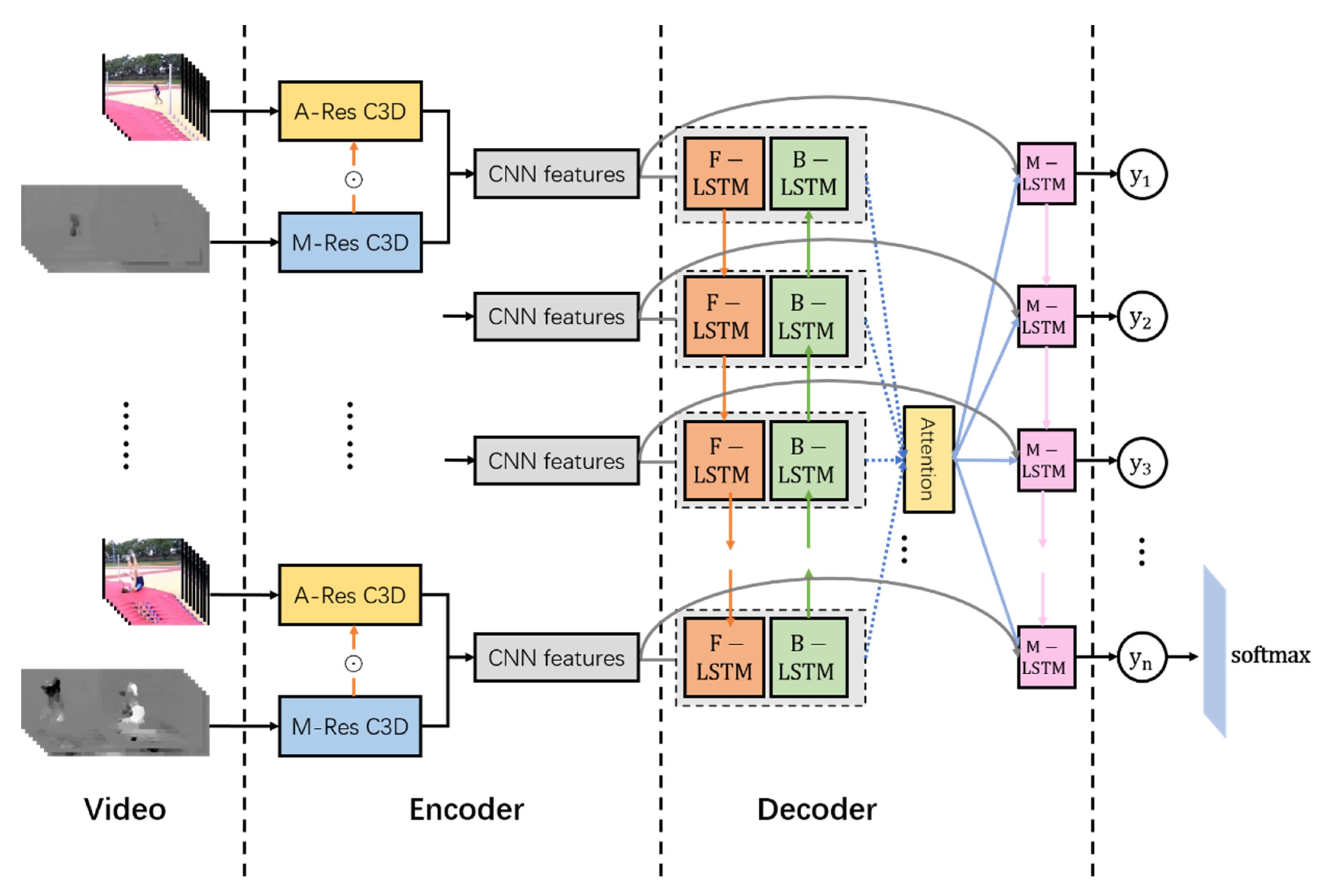
In this paper, we introduce an encoder–decoder framework named Two-Stream BiLSTM Residual Network (TBRNet) for video action recognition. More specifically, in the encoding phase, in contrast to the original two-stream network that extracts appearance and motion features separately, our proposed two-stream encoder consisted of a spatial appearance stream and a temporal motion stream with multiplicative residual connections inserted between the two pathways. These connections affect the gradients and make the hierarchical spatiotemporal features interact earlier during processing. Moreover, the two pathways were constructed by proposed 3D CNN named Res-C3D network, which has 3D convolution kernels with residual blocks. Then, the spatial appearance features and temporal motion features from the fully connected layers of each pathway were fused together as short-term spatiotemporal representations of the encoder. In the decoding phase, the fused representations at every time step were sent to the temporal attention-based BiLSTM network which models the temporal dependencies for sequences in both the forward and backward directions and concentrates more on salient information. After that, the temporal dependencies were integrated with short-term spatiotemporal features by residual connections and then sent to another LSTM network, followed by a softmax classifier for the final prediction of the video action. Ablation experiments on two video action recognition datasets, named UCF101 and HMDB51, proved the effectiveness of our approaches. Our proposed model not only showed significant improvements over baseline models but also outperformed some state-of-the-art methods. To summarize, the contributions of this work are as follows:
We accurately modeled the interactions between spatial and temporal features using proposed a two-stream encoder with cross-stream residual connections which were also benefit for backpropagation of gradients;
We effectively captured the global spatiotemporal dependencies by incorporating the local features in a fixed-length window extracted by proposed Res-C3D and the long-term relationships among entire sequences extracted by proposed attention-based BiLSTM;
We proposed a new model with encoder–decoder framework named TBRNet for video action recognition. Extensive experiments on two benchmark datasets named UCF101 and HMDB51 show the effectiveness of our proposed model, and it achieves competitive or even better results compared with some existing state-of-the-art approaches.
The rest of the paper is organized as follows: In
Section 2, related works of ours are briefly reviewed. In
Section 3, we introduce our proposed framework TBRNet. Introduction of datasets and implement details, ablation study and the comparison with state-of-the-art approaches are discussed in
Section 4.
Section 5 concludes the paper.
3. Proposed Approach
In this section, we describe our proposed TBRNet and its main components. The TBRNet can be divided into two modules: the two-stream CNN-based encoder and the BiLSTM-based decoder. The overall architecture of TBRNet is shown in
Figure 3. Specifically, residual learning, as well as its key idea, is described in the first subsection, since it is applied to three places in our model. Then, we introduce the proposed Res-C3D model which is used to construct the two streams. After that, several types of interaction between the two pathways are discussed. Subsequently, we describe the decoder modeled with the BiLSTM network. Finally, the attention mechanism for BiLSTM and the integration of overall global spatiotemporal representations using residual connections are described in the last subsection.
3.1. Residual Network
Evidence [
7,
41] has revealed that with the increasing depth of a CNN, more hierarchical features can be integrated from deep networks, which translates to a more powerful ability to obtain semantic information. However, only increasing the number of network layers leads to the problem of vanishing gradients, which hampers the convergence from the start and ultimately results in the degradation of accuracy. To avoid this problem, we built our network by taking advantage of the idea of shortcut connections. Instead of using a “highway network” [
42,
43], weighted residual terms are replaced with identity mapping. As shown in
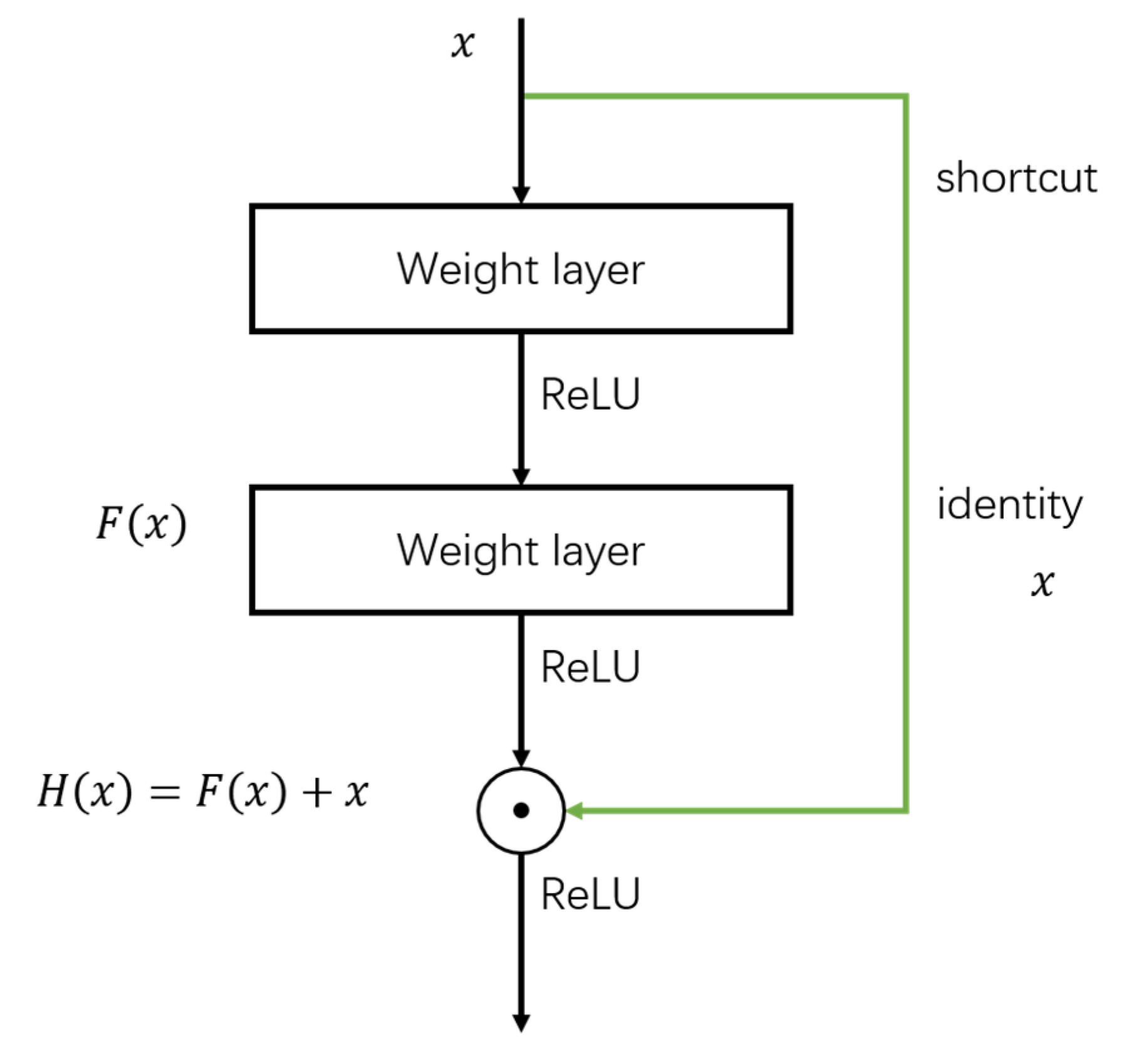
Figure 4, through the “shortcut” skipping connections, the input signal can be directly propagated to any later layer of the network as the output.
where
is the input vector of the considered layer,
is the desired underlying mapping,
denotes the convolution filter weights matrix, and the function
stands for the nonlinear residual mapping needed to learn. If we want to fit the underlying mapping
by a few stacked layers, we let these layers approximate another mapping
, and then the original mapping is recast into
, which is easier to learn and better for network optimization.
By introducing skipping connections, the residual learning has the advantages of not only maintaining the features from former layers while learning new information but also propagating gradients from the loss layer directly to any former layers during backpropagation. Thus, the problem of degradation as the network depth increases can be mitigated.
3.2. Two-Stream Interaction
In the original two-stream architecture, a video is represented as an RGB frame and a stack of optical flow frames, which are separately fed into the appearance stream and motion stream. Each of the two processing paths generates the spatial and temporal features on its own to obtain the softmax predictions which are averaged in the last step to calculate the final results of classification. Since this architecture extracts the appearance and motion features in parallel and has no interaction before the final fusion, it is incapable of modeling the subtle spatiotemporal cues, which are of significant importance for distinguishing videos that have similar appearances or motion patterns.
In our work, a video was first represented as small segments, where also corresponds to the time steps of the BiLSTM decoder. For each segment, we sampled RGB frames and the corresponding optical flow frames. One stack of RGB frames and optical flow frames covering one local video segment were fed into the appearance and motion streams, respectively, which had the same CNN structure for modeling the correlations of appearance and motion features between the same abstract levels of two streams.
Several types of cross-stream connection [
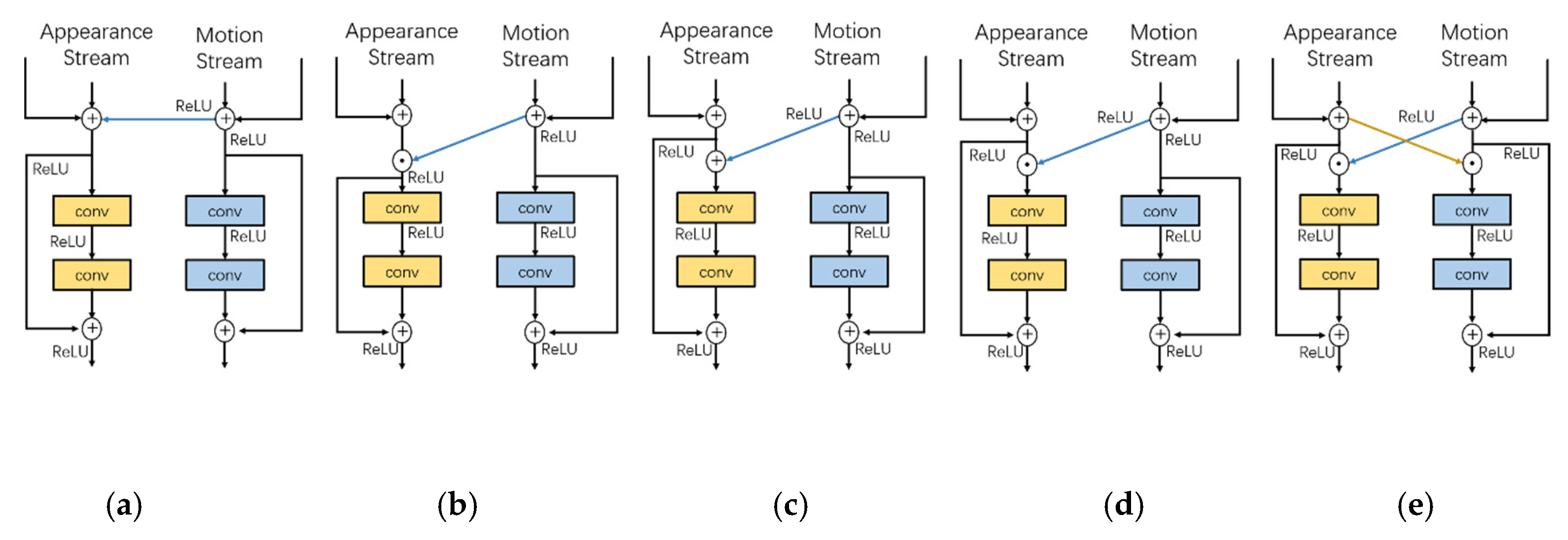
39] can be introduced between the identical abstraction levels of the two pathways for an earlier interaction as depicted in
Figure 5. However, the performances of structures with a simple direct connection, such as those shown in
Figure 5a,b, are inferior to others, which is imputed to the huge changes in distribution directly induced by the other stream.
As depicted in
Figure 5c, the additive connections injected from the motion stream to the appearance stream can be formalized as:
Here,
and
stand for the inputs of the
th layer of the appearance and motion streams, respectively,
stands for the inputs of the
) th layer of appearance stream, and
denotes the weight matrix of this unit in the appearance stream.
denotes ReLU activation function, and
denotes the operators of convolutional layers and ReLU activation layers shown in above figures. Then, during the backpropagation, given the inputs of the
)th layer of motion stream
, the gradient of the loss function
of the appearance stream
and motion stream
can be calculated through the chain rules as:
Similarly, as depicted in
Figure 5d, applying the multiplicative motion gating to two streams can be formalized as:
Here,
denotes element-wise multiplication. Correspondingly, the gradient of the loss function
of the appearance stream in the backpropagation is formulated as:
where the gradient of residual unit is modulated by the signal
from the motion stream.
The loss function
of the motion stream is similarly calculated as:
where the gradient of the residual unit is modulated by the signal
from the appearance stream and is added to the gradient of the motion stream
to become the gradient of the loss function
of the motion stream.
Finally, as depicted in
Figure 5e, the bidirectional multiplicative residual connections can be considered as the multiplicative motion gating and multiplicative appearance gating applied on appearance stream and motion stream respectively, and the multiplicative appearance gating is similar as the motion gating discussed above.
As a result, the signals from each of the streams can be involved together and then affect the gradient during the backpropagation, which helps mitigate the problem of the original two-stream network’s deficiency in modeling the subtle spatiotemporal correlations.
3.3. Res-C3D Network
We built each stream on the basis of 3D CNN with residual blocks instead of 2D CNN. We utilized C3D [
4] as the base model which was equipped with 3D convolution kernels to directly extract the hidden patterns from a stack of RGB or optical flow frames ordered by time sequences. Therefore, it was an effective feature learning network for modeling the spatial features together with the local short fixed-range temporal relationships.
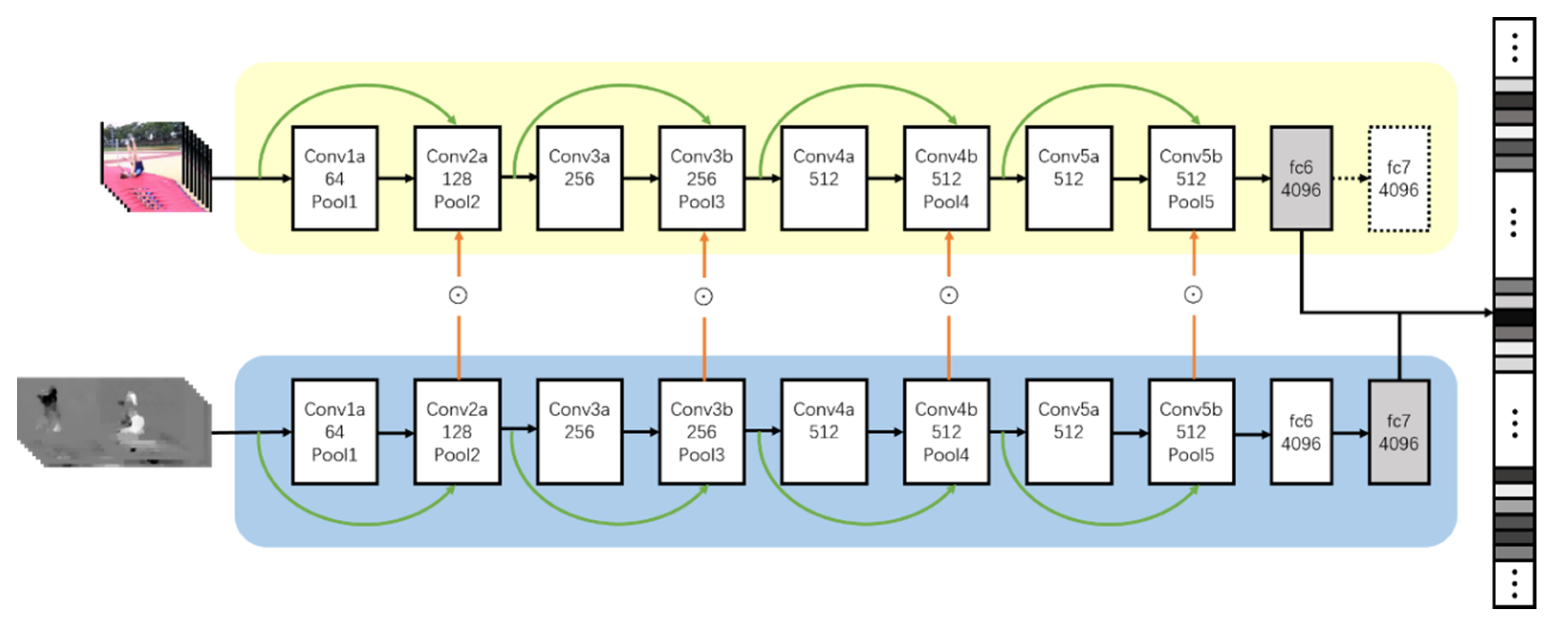
The original C3D model had five convolution blocks with eight convolution layers, five pooling layers, two fully connected layers, and a softmax loss layer. All the convolution layers had 3 × 3 × 3 convolution kernels with stride 1 × 1 × 1. The channel size for each convolution block was set to 64, 128, 256, 512, and 512 from the first block to the fifth block. The second to the fifth pooling layers all had 2 × 2 × 2 pooling kernels with stride 2 in both the spatial and temporal dimensions in order to downsample the feature maps by a factor of eight The first pooling layer had a kernel size of 1 × 2 × 2, which was designed for preserving the temporal signals in the early steps. The two fully connected layers had a 4096 dimensional output size, followed by a softmax classifier to obtain the prediction results.
We generalized the idea of identical mapping with residual connections for the original C3D network and constructed an identical mapping “shortcut” by introducing residual connections between convolution blocks, which are depicted as the green curved arrows in
Figure 6. These residual blocks are capable of preserving network performance by maintaining the learned features via identical mapping and integrating newly learned patterns to optimize the spatiotemporal representations.
Finally, considering that the fully connected layer was capable of perceiving the entire model so as to obtain high-level semantic information, we merged the outputs of the fully connected layers from two streams together to be the short-term spatiotemporal features of encoder. Since the deeper fully connected layers contained stronger signals, fc6 of appearance stream and fc7 of motion stream were combined together, and this type of combination strategy achieves better result compared to others. It can be explained by the fact that it is better to contain appearance signals with less strength and make the motion signals predominate during the training process.
3.4. BiLSTM Network
Owing to the recurrent connections of each unit, RNNs yield good performances in modeling hidden sequential patterns of data. However, the “internal memory” property and the “vanishing gradient” problem of the RNN recurrent structure make it difficult to update the network parameters during backpropagation; thus, RNNs are deficient in interpreting early information and modeling the long-range temporal contexts of feature vector sequences.
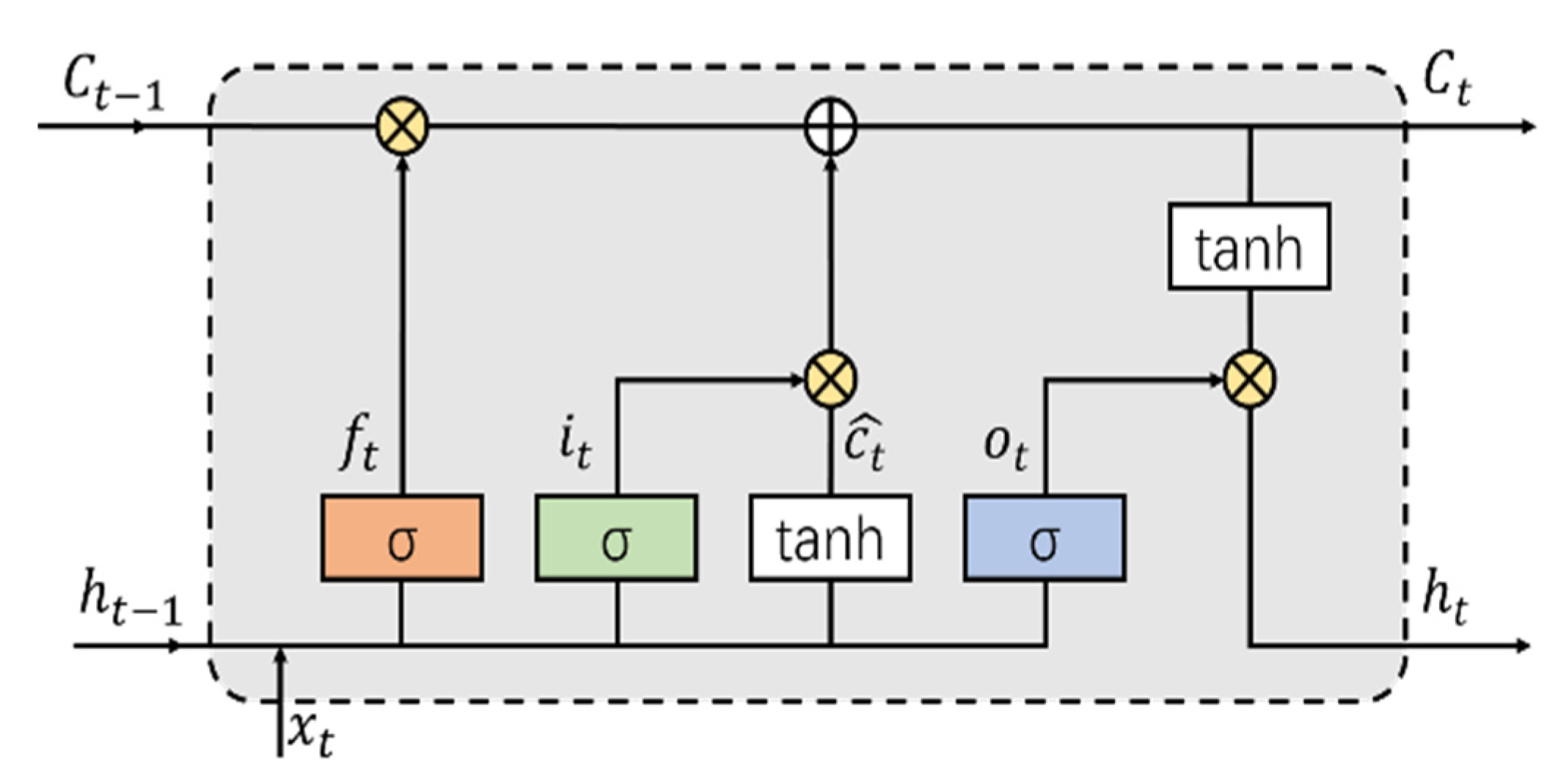
Fortunately, LSTM conquers this fundamental weakness through its unique cell structure, which contains forget, input, and output gates controlled by sigmoid units to decide what information to update and store in memory cells. Linear connections across these LSTM units help to transmit the previous information to the present time step. The structure of an LSTM unit is illustrated in
Figure 7.
Given the current input vector
, the last hidden state
, and the last memory cell state
, the operations inside the LSTM cell can be formulated as
where
,
,
, and
denote the input gate, forget gate, output gate, and input modulation gate at time
, respectively.
,
, and
denote the input weights, recursive weights, and bias vector.
denotes the sigmoid activation function, and
denotes the hyperbolic tangent function.
is a vector that offers candidate values to update the memory cell, which is calculated from the present input and previous state by the
activation function. The input gate
and the input modulation gate
control what to write to the memory cell, while the forget gate
controls what previous information transmitted from the past to discard. The output gate
keeps the information for forthcoming operations that control the output of the cell at time
. After updating the memory cell as
, the hidden state
at time
can be calculated by element-wise multiplication of the output gate vector
and current memory cell state
after projection by the
function.
Stacking two LSTM layers of opposite directions together in our network serves as the point of departure for the use of the bidirectional temporal structures of feature vector sequences. In contrast to the outputs of standard single-layer LSTM at time , the combined outputs of BiLSTM layers are decided by not only the cues from previous vectors but also cues from upcoming vectors. Therefore, by integrating the extra information from future data, BiLSTM networks are capable of generating higher-level global context relationships of sequential data from videos.
The CNN feature vectors from the encoder serve as the visual representations of each video clip, which are ordered as temporal sequences. Venugopalan et al. [
27] employed the LSTM network to model the temporal dependencies of the features, which can be expressed as:
where
indicates the feature vectors modeled at time
,
denotes the temporal information, and
denotes the modeling function for temporal relationships.
In contrast to Equation (14), which only takes the past information into consideration, in our work, we employed the BiLSTM network to abstract the temporal representation of both past and future information separately, and two hidden states of LSTM were merged to become the output, which can be illustrated as:
In other words, by employing the BiLSTM network in our model, the long-term bidirectional global temporal relationships were abstracted by going forward and backward several times through the vector sequences encoded from all the video segments.
3.5. Temporal Attention Mechanism
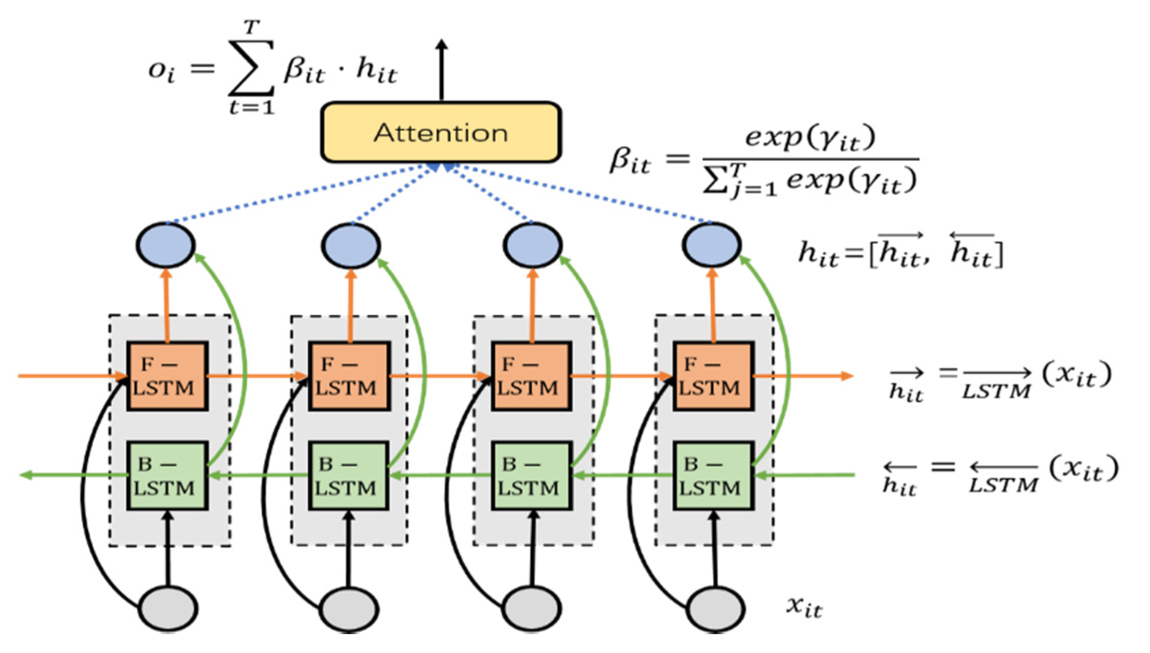
When we are looking at a dog, we usually focus on the body of the dog and try to observe it clearly while roughly glancing at other regions, such as the background. The attention mechanism is first implemented as a spatial version for image perception, which directs the visual attention to the salient part of images and pays less attention to other useless areas. Similarly, the contribution provided by every single input element from sequential data to abstract semantic content is not equal. For example, the start and the end segments of videos usually carry less vital information compared with some key segments located in the middle of videos. The principle of the temporal attention mechanism is to decide “when” to look by automatically directing high levels of focus to those vectors that contain the most valuable information while directing relatively low-level focus to those containing less information according to the importance and relevance of the tasks. In our work, we employed the temporal attention mechanism in the BiLSTM network to simulate the process of focusing attention among all segments of videos, where the gradients of the loss function of BiLSTM can be backpropagated through both the BiLSTM network and the attention network.
The BiLSTM with the temporal attention mechanism is depicted in
Figure 8. Specifically, given the input vector
, where
, the hidden state of each time step encoded by BiLSTM can be formulated as
where the forward and backward directions of the input sequences are denoted as ← and →, respectively. The final hidden state of BiLSTM can be expressed as:
Then, the attention-based temporal attribute vector
is calculated by the weighted average:
Here,
denotes the attention weights of the
-th BiLSTM output vector at time
, which is computed by the following equations:
where
is the weight matrix used to project the current input
of BiLSTM into another space, and
is a bias vector. We utilize the nonlinear
activation function for the frame selection gate as the relevance vector
and normalize it through a softmax function. In other words, the temporal attention mechanism can be learned as a special representation of the time steps of interest to restrain the redundancy and noises.
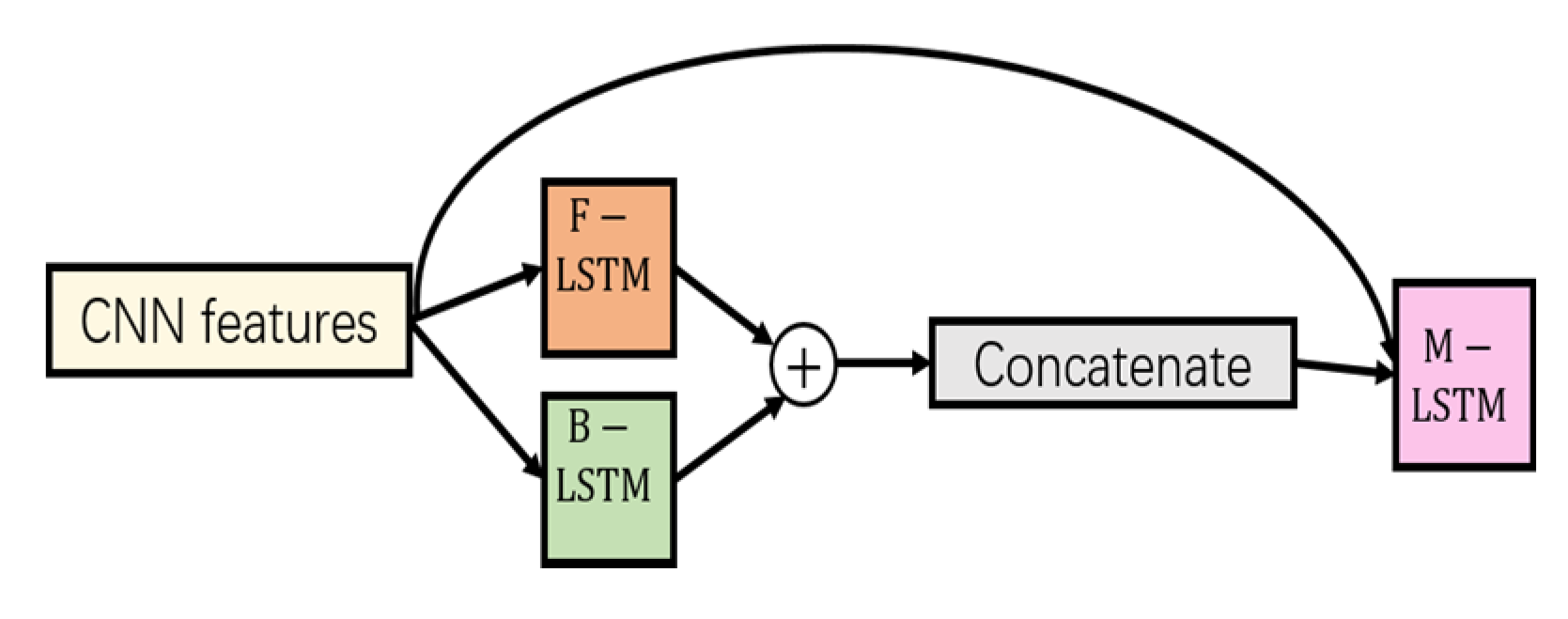
Then, we employed another LSTM for the final representations of videos by taking the integration of the CNN visual features extracted by the encoder and the merged outputs of BiLSTM together as inputs. As illustrated in
Figure 9, there is an identical mapping residual connection from the output layer of the encoder to the bidirectional representations, which constructs a highway between layers and is thereby more conducive to gradient propagation through the network and the abstraction of global spatiotemporal representations.
4. Experiments
In this section, our proposed network is evaluated on two benchmark datasets named UCF101 and HMDB51 for video action recognition. In the first part, we introduce these two datasets and the implementation details of our experiments. An ablation study for demonstrating the effectiveness of our proposed method is described in the next part. In the last part, we compare our TBRNet with state-of-the-art approaches.
4.1. Datasets and Implement Details
Created by Florida University, the UCF101 dataset is one of the most challenging datasets for video action recognition in realistic scenes, where the videos are captured with a large diversity of poses, viewpoints, illumination conditions, and cluttered background. It contains 13,320 videos with a spatial resolution of 320 × 240 that can be categorized into 101 classes. Each class includes 100–200 videos, and these classes of action are divided into five types: (1) human–object interaction, (2) body motion only, (3) human–human interaction, (4) the playing of musical instruments, and (5) sports.
The HMDB51 dataset, a more challenging dataset published by American Brown University in 2011, contains more than 6000 video clips in total. The videos are organized as 51 distinct classes of action, and each class has more than 100 clips. The dataset covers highly diverse actions, such as object manipulations, facial actions, body movements, and human interactions. Problems such as poor video quality, a small number of training videos, significant camera motion, and a complex dynamic environment lead to higher intra-class variation, which makes it more challenging to reduce errors during training and testing periods. For both datasets, we adopted the original training/test splits and followed the standard evaluation protocols provided by the authors of these two datasets by averaging the accuracies of three splits as the final result.
For the two-stream CNN encoder, we adopted the pre-computed RGB and optical flow frames of videos from Reference [
3] as the inputs of our model. We divided each video into
segments, which also relates to the time steps of the BiLSTM decoder sequences. We sampled
frames of RGB frames and the corresponding
optical flow frames for each segment and used them as the input modalities. The settings of
and
are based on our experiments, which show optimal results in complexity and accuracy. Since the number of videos provided by datasets is limited, we adopted the same data augmentation strategy as [
4] to mitigate the effect of overfitting. We resized the frame to 128 × 171 and randomly cropped them into 112 × 112. Thus, one input segment has a size of 8 × 112 × 112. Additionally, we horizontally flipped them with a 55% probability to further augment the training samples.
As UCF101 is a larger dataset than HMDB51, we first trained our two-stream encoder on UCF101 to extract visual CNN features and then transferred it for HMDB51. As depicted in
Figure 6, the merged output of fc6 from the appearance stream and fc7 from the motion stream were used to represent features of a video segment, which is a vector of 8192 dimensions. For each video, 12 feature vectors were fed into BiLSTM with 8192-dimensional hidden states. The outputs of the BiLSTM network with a weighted sum attention pooling were fed into another LSTM, together with the CNN visual features, to obtain the final global spatiotemporal representations. In the end, those spatiotemporal representations were optimized by the softmax cross-entropy loss to predict the actions.
We trained the model with the stochastic gradient descent (SGD) algorithm and set the batch size to 32 to perform the batch normalizations because of the memory constraints. The learning rate was set to 0.01 in the first 2000 iterations and then lowered at a fixed ratio every 100 iterations. For better training and validating, we also applied a momentum of 0.9 and an early-stopping strategy during the process of training. In addition, we applied a dropout probability of 0.8 to the fully connected layers in the encoder and also applied the decoder with a dropout of 0.5 to bidirectional connections.
4.2. Ablation Study
4.2.1. Analysis of Res-C3D Network
We first evaluate the performance of our proposed Res-C3D with residual connections by using the performance of C3D as a comparison.
Table 1 shows the classification accuracies on UCF101 and HMDB51 for the different pathways employed with these two networks. By introducing residual blocks, our proposed Res-C3D outperformed the C3D not only in the single stream but also in the two-stream architecture. Especially, when applied to the motion stream, the proposed Res-C3D achieved a 3.7% increase in accuracy on HMDB51. Therefore, the residual learning of Res-C3D proved to be beneficial for feature generation which can be attributed to better signal propagation, especially the backward propagation during the training process.
Table 1 also shows that the two-stream network architecture outperforms by a large margin compared with the single-stream architectures because it is capable of appropriately taking advantage of the information from both streams to model the spatiotemporal features rather than only using the information from a single one.
4.2.2. Analysis of Cross-Stream Connections
For the purpose of learning the correspondences between the appearance and motion signals from identical levels of abstraction in the two streams, we introduced cross-stream connections into the two-stream network. Generally, as shown in
Figure 5, there are several possible variants of connections for interactions between pixels at the same position of the two processing pathways. We use the classification errors on UCF101 and HMDB51 to evaluate the performances of these different types of interaction; as shown in
Table 2, a lower value of error represents a more appropriate model. In
Table 2,
denotes the additive operation, while
denotes the element-wise multiplicative operation. In addition, we use ← and → to denote the direction of flow from the motion to the appearance stream and its opposite direction, respectively, and use ←→ to represent the bidirectional connection between the two streams.
Firstly, we used the direct additive and multiplicative shortcut for cross-stream connections, as illustrated in
Figure 5a,b. In the two-stream architecture equipped with the proposed Res-C3D, these kinds of structures allowed for the straightforward flow of the motion signals via the residual connections of each Res-C3D in both pathways, which, however, introduce large changes in input distribution into the appearance pathway. Those changes not only flow through the forward processing procedure to reach the deep layers but also are backpropagated to former layers after fusing with appearance features, thus resulting in the disturbance of the network capability of pattern encoding. In other words, the straightforward shortcuts damaged the identity mapping of the original residual signal flow of the appearance Res-C3D, which increased the difficulty of optimization and increased the classification errors as listed in the first two rows of
Table 2. We also note that the performance of the direct multiplicative shortcut connection is even worse compared with that of the additive shortcut connection. The explanation for this is that employing multiplicative operations on a straightforward connection amplifies the impacts of disturbing basic feature extraction on the two pathways. The results are similar when applying the connections from the appearance stream to the motion stream. Therefore, we continued the following experiments not based on the simple direct interactions but on the cross-stream residual connections illustrated in
Figure 5c,d,e.
Secondly, we compared the additive and multiplicative operations for cross-stream residual connections, which were introduced in
Section 2. As we can see from
Table 2, using multiplicative gating from the motion to the appearance stream led to errors of 7.53% and 36.69% on UCF101 and HMDB51, and additive gating achieved slightly worse results with errors of 9.04% and 39.91%. The multiplicative residual connections strengthen the information correspondences of the two pathways by modulating the gradient propagation with signals from both pathways. This type of reinforcement of two signals from each stream improves the ability of the two-stream encoder to learn spatiotemporal features.
Thirdly, we evaluated the performances of employing different directions of cross-stream connections in our network. As we can see from rows 4, 6, and 7 of
Table 2, under the circumstance of multiplicative gating, the fusing direction from the motion to the appearance stream achieves superior performance compared with the other two types. Similar to the additive gating (rows 3 and 5 of
Table 2), letting the motion signals flow to the appearance stream outperforms the same schema but in the opposite direction. Since the appearance features have stronger effects on recognizing the hidden patterns in frames, when enabling the flow of appearance signals to the motion stream, the whole network is dominated by appearance signals, which makes the loss of motion stream quickly reduce to a low value and finally leads to the overfitting to appearance patterns. Things are different when using the ← direction, where both pathways learn the motion patterns together without suffering from the overfitting resulting from the domination of motion signals, thus modeling more appropriate spatiotemporal features. In the ←→ bidirectional connections, the same problem occurs in which the appearance signals flowing in both streams force the whole network to overemphasize appearance information from RGB frames.
Therefore, we employed the multiplicative cross-stream residual connections illustrated in
Figure 5d with a fusion of directions from the motion to the appearance stream for the two-stream CNN encoder, which is verified to be more effective for extracting spatiotemporal features than other variants.
4.2.3. Analysis of Fusion Strategies
Table 3 shows the results of fusing two signals from different layers of the appearance and motion streams. Fusing the last convolution layer of the two pathways had inferior performance compared with the fusion of fully connected layers because the fully connected layers are capable of perceiving the overall model so as to obtain higher-level semantic information. Fusing both fc7 layers from each stream outperformed the fusion of both layers to fc6, which demonstrates that the fusion of deeper layers led to deeper patterns of spatiotemporal representations extracted by more layers. However, the combination of fc6 of the appearance stream and fc7 of the motion stream achieved the best result among these fusion modalities, which can be explained by the fact that it is better to contain appearance signals with less strength and make the motion signals predominate during the training process by utilizing representations from lower fully connected layers of the appearance stream and deeper fully connected layers of the motion stream.
4.2.4. Analysis of Attention-Based BiLSTM
In
Table 4, we evaluated the performances of different variants of the visual representation decoder by using the sequential features from the two-stream CNN encoder as inputs. The result showed that adding the LSTM network was beneficial for decoding the long-term visual representations into temporal dependencies because of its capability of “remembering” information, which yields margins of at least 1.3% and 3.1% on UCF101 and HMDB51. Furthermore, the bidirectional structure outperformed the unidirectional LSTM structure, because it provides double temporal contexts by gathering information from both previous and future segments. Additionally, the temporal attention mechanism was applied to the LSTM network, and the results verified that with the additional temporal attention layer, both unidirectional and bidirectional LSTMs, performed better than the LSTMs without the attention mechanism. This was because the temporal attention mechanism simulates the attention of humans by focusing less on unimportant video segments and concentrating more on salient parts by assigning different attention weights.
We also compared the performance of using the residual connection to integrate CNN visual representations with BiLSTM temporal relationships as depicted in
Figure 9. From the comparison of the last two rows of
Table 4, we noticed that the network with the residual connections achieved higher accuracy, and we attribute this improvement to the better propagation of global spatiotemporal representations within the whole network resulting from the overall fusion.
4.3. Comparison with State-of-the-Art Models
In this section, we compare our proposed model with existing state-of-the-art video action recognition approaches on both UCF101 and HMDB51 benchmark datasets. We categorize these approaches into three types according to the types of extracted features, as reported in
Table 5.
Compared with the approaches that use hand-crafted features [
17,
44], our proposed TBRNet yielded significant margins as high as 9.5% and 15.6% on UCF101 and HMDB51.
Our encoder of TBRNet was based on a two-stream network [
2] and C3D [
4] which outperformed these two base models by 4.0% and 6.8% on UCF101. We note that some two-stream-based approaches, such as Two-stream fusion [
3] and Spatiotemporal ResNets [
38], lead to higher accuracies compared with our proposed two-stream encoder, and this can be explained by the fact that these two approaches with similar fusion strategies among streams use deeper CNNs as base models which need to learn more network parameters. However, with the help of the temporal attention-based BiLSTM decoder, our entire TBRNet achieved improvements of 2.9% and 2.0% on UCF101 and 7.4% and 6.4% on HMDB51, which verifies the benefit of our decoder in capturing long-term dependencies for temporal sequences. Compared with other 3D CNN methods, such as 3D Convolution [
12], Res3D [
26], and other LSTM-based methods, such as LSTM [
5], LRCN [
6], Two-stream + LSTM [
28], and Multi-LSTM [
45], our proposed TBRNet still performed better.
From the performances of approaches that use hybrid features, such as TDD [
44], C3D, and 3D Convolution, higher accuracies were obtained by taking iDT into consideration. Dense trajectories, calculated by the iDT algorithm, were stronger representations that contained more spatiotemporal features. However, they require higher computation resources compared with the usage of only optical flow. Note that without the BiLSTM decoder to model the long-range temporal dependencies, our two-stream CNN encoder still outperformed C3D and TDD with iDT versions by 1.6% and 0.5% on UCF101, which shows the strong ability of our proposed encoder to capture spatiotemporal features from RGB frames and optical flow frames in a fixed-length temporal window. In addition, TSN [
19] with iDT is pre-trained with the help of a large-scale ImageNet dataset which provides high diversity for training. Despite that, our proposed TBRNet also showed superior performance.
Finally, we demonstrate that our TBRNet with an encoder–decoder framework provided global spatiotemporal information complementarily and achieved classification accuracies of 95.4% and 72.8% on UCF101 and HMDB51.
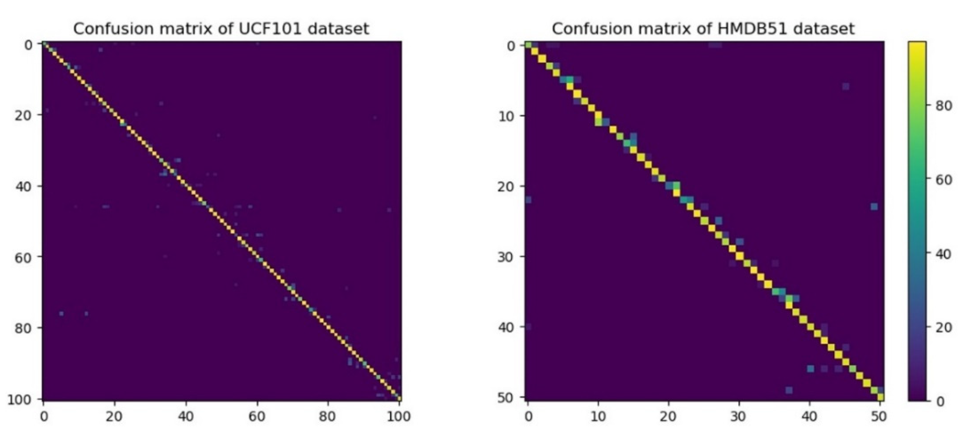
The performances for all action classes in UCF101 and HMDB51 are given in
Figure 10, and these confusion matrixes are well diagonalized. Some categories are easy to recognize, such as “pull-up” and “ride bike” in HMDB51, “BenchPress” and “BandMarching” in UCF101. However, some categories are hard to recognize, such as “laugh” in HMDB51 and “ApplyLipstick” in UCF101, since the videos in “ApplyLipstick” are easily confused with “ApplyEyeMakeup” and “BrushingTeeth”. Nonetheless, our proposed model still performs well with most categories.
Some correct and misclassified examples of the prediction results are shown in
Figure 11a and
Figure 11b, respectively. We used the top two categories scores predicted by our TBRNet. It can be seen that similar actions can disturb the prediction of classifiers. For example, in the particular video, the action “Cartwheel” looks like “HandupStand”, which makes our classifiers confused. We attribute the misclassification of these actions to their high within-class variance and low between-class variance to their targeted false class.


