Application of Generalized Polynomial Chaos for Quantification of Uncertainties of Time Averages and Their Sensitivities in Chaotic Systems

Abstract

In this paper, we consider the effect of stochastic uncertainties on non-linear systems with chaotic behavior. More specifically, we quantify the effect of parametric uncertainties to time-averaged quantities and their sensitivities. Sampling methods for Uncertainty Quantification (UQ), such as the Monte–Carlo (MC), are very costly, while traditional methods for sensitivity analysis, such as the adjoint, fail in chaotic systems. In this work, we employ the non-intrusive generalized Polynomial Chaos (gPC) for UQ, coupled with the Multiple-Shooting Shadowing (MSS) algorithm for sensitivity analysis of chaotic systems. It is shown that the gPC, coupled with MSS, is an appropriate method for conducting UQ in chaotic systems and produces results that match well with those from MC and Finite-Differences (FD).

1. Introduction

Over the past few decades, modern computational methods have been very successful in predicting the evolution of systems of great complexity. However, in real–life applications, the system behavior is significantly affected by parametric uncertainties. As an example, geometric uncertainties in the shape of the front wing, diffuser, and the tip of a Formula (1) can affect its performance [1]. A small selection of other examples can be found in References [2,3,4,5].

Various techniques for the quantification of uncertainties have been developed. These include sampling techniques, such as the Monte-Carlo [6], Latin Hypercube sampling [7], and quasi Monte–Carlo [8]. However, despite their accuracy and ease of application, these methods become computationally intractable for large, real world problems, such us high fidelity simulations of turbulent flows. Other approaches, based on the spectral representation of uncertain quantities, have also been developed. These techniques are referred to as Polynomial Chaos Expansion (PCE) methods. They were first developed in Reference [9] for Gaussian uncertainties, and, later in Reference [10], they were generalized for all Probability Density Functions (PDFs) in the Askey scheme. The ability of generalized PCE (gPC) in quantifying uncertainties has been amply demonstrated in many applications, for example, in Computational Fluid Dynamic (CFD) systems [11,12,13]. Recent developments in Uncertainty Quantification (UQ) include using the PCE in data-driven approaches [14]. Spectral approaches are computationally efficient for a small number of uncertain parameters, m, but their cost increases exponentially with m (curse of dimensionality).

There are two major approaches to applying gPC, the intrusive (iPC) [5,15] and the non-intrusive (niPC) [16]. In the intrusive approach, the state vector is written in spectral form using the gPC, and a new set of state equations, the iPC equations, are extracted using Galerkin projection. On the other hand, the non-intrusive approach is based on the spectral representation of a Quantity of Interest (QoI), such as the lift of an airfoil, and the spectral coefficients are calculated by repeated evaluations of the QoI at specific quadrature locations.

For general unsteady systems, the iPC approach is not feasible for conducting UQ because the accuracy of the spectral representation of the state variables starts to deteriorate after the system starts to evolve from the initial condition. For this reason, we used the niPC approach and focused on uncertainties of time-averaged quantities and their sensitivities with respect to input parameters. Time-averaged quantities are of interest to many engineering applications, for example, in aeronautics (lift and drag around an airfoil), energy generation (fuel consumption and pollutant formation), process industries (average heat transfer, mixing rate), etc.

Although time-averages of state variables can be easily computed by collecting statistics over long time integration, the evaluation of their sensitivities to input parameters is much more involved. The adjoint sensitivity analysis approach [17] is based on a linearization of the evolution equation with respect to one or more system parameters. This approach, however, breaks down in chaotic systems, where the state variables display extreme sensitivity to minute variations in input conditions [18]. In such cases, the adjoint variables diverge; this is popularly known as the ‘butterfly effect’, and it is due to the presence of one or positive Lyapunov exponents.

The Least-Squares Shadowing (LSS) approach was developed in Reference [19] and resolves this problem. It is based on the shadowing lemma for ergodic and uniformly hyperbolic dynamical systems [20]. Although computationally expensive, the method can give values for the sensitivities of time-averaged quantities that match well with finite differences. In this work, the preconditioned Multiple-Shooting (MSS) [21,22], a computationally more efficient version of the LSS, is used to evaluate sensitivities of time-averages.

In this paper, it is shown that the non-intrusive approach to the gPC is suitable for UQ of time-averages of chaotic systems and their sensitivities, with respect to system parameters. Information on the latter, i.e., UQ of sensitivities, is important in robust design applications, where the expectation of a QoI is minimized under uncertainty. The present work follows on from previous work of the authors in this area [23].

2. Sensitivity Analysis of Chaotic Systems Using MSS

In this work, we consider a non-linear dynamical system governed by the equation

$$\frac{d\mathbf{u}}{dt}=\mathbf{f}(\mathbf{u},\mathbf{s}),$$

(1)

where $\mathbf{u}$ denotes the state vector, and $\mathbf{s}$ a set of design parameters. This is a set of ordinary differential equations (ODEs) that arise after spatial discretisation of partial differential equations (PDEs). The QoI is the time average of some function $G(\mathbf{u},\mathbf{s})$ of the state variables and design parameters, as in

$${\overline{G}}_{\infty }\left(\mathbf{s}\right)=\underset{T\to \infty }{lim}\frac{1}{T}{\int }_0^{T}G(\mathbf{u},\mathbf{s})dt.$$

(2)

An example QoI from the field of aerodynamics is the time-average of the lift or the drag coefficient of an airfoil.

The conventional adjoint sensitivity analysis to determine $\frac{d{\overline{G}}_{\infty }\left(\mathbf{s}\right)}{d\mathbf{s}}$ requires the formation of the augmented Lagrangian

$$\Lambda =\frac{1}{T}{\int }_0^{T}G(\mathbf{u},\mathbf{s})+{\lambda }^T\left(\frac{d\mathbf{u}}{dt}-\mathbf{f}(\mathbf{u},\mathbf{s})\right)dt+{\mu }^T\left(\mathbf{u}\left(0\right)-{\mathbf{u}}_0\right).$$

(3)

After differentiation with respect to $\mathbf{s}$ and integration by parts, we arrive at the adjoint system

$$\frac{d\lambda }{dt}=-{\left(\frac{\partial \mathbf{f}}{\partial \mathbf{u}}\right)}^T\lambda +\frac{\partial G(\mathbf{u},\mathbf{s})}{\partial \mathbf{s}},$$

(4)

which is integrated backwards in time with terminal condition $\lambda \left(T\right)=0$. As mentioned in the Introduction, if the system in Equation (1) is chaotic and has at least one positive Lyapunov exponent, then marching Equation (4) backwards will result in an exponentially growing adjoint state vector $\lambda$.

To resolve the problem of diverging trajectories for $\mathbf{s}$ and $\mathbf{s}+\delta \mathbf{s}$, we formulate a minimization problem that keeps the two trajectories close in phase space. To achieve this, we relax the requirement of fixed initial condition for the two nearby values of $\mathbf{s}$. However, for ergodic systems, this change does not affect the time-average values and their sensitivities. Below, we state the minimization problem for a single parameter s, but an adjoint version for multiple parameters can be also formulated.

$$\begin{array}{cc}\hfill \underset{\mathbf{v}\left(t_i^{+}\right)}{\min }\sum _{i=0}^K{\parallel \mathbf{v}\left(t_i^{+}\right)\parallel }_2^2& ,\hfill \end{array}$$

(5a)

$$\begin{array}{cc}\hfill \mathrm{subject}\mathrm{to}\mathbf{v}\left(t_i^{+}\right)=\mathbf{v}\left(t_i^{-}\right)& ,\hfill \end{array}$$

(5b)

$$\begin{array}{cc}\hfill \frac{d\mathbf{v}}{dt}-\frac{\partial \mathbf{f}}{\partial \mathbf{u}}\mathbf{v}-\frac{\partial \mathbf{f}}{\partial s}-\eta \mathbf{f}=0& ,\hfill \end{array}$$

(5c)

$$\begin{array}{cc}\hfill \langle \mathbf{f}\left(\mathbf{u}\right(t),s),\mathbf{v}\left(t\right)\rangle =0& ,\hfill \end{array}$$

(5d)

$$\begin{array}{c}\hfill \mathrm{where}{t}_i<t<t_{i+1}(i=0,...,K-1),\end{array}$$

(5e)

where

$$\begin{array}{cc}\hfill & \mathbf{v}\left(t\right)=\underset{\delta s\to 0}{lim}\frac{\mathbf{u}(\tau (t);s+ds)-\mathbf{u}(t;s)}{\delta s}\hfill \\ \hfill & \eta \left(t\right)=\frac{d}{ds}\left(\frac{d\tau \left(t\right)}{dt}-1\right).\hfill \end{array}$$

(6)

The objective to be minimized, given in Equation (5a), is the $L_2$ norm of the distance between the two trajectories in phase space. This norm is computed using the distance at $K+1$ discrete time points $t_0,\cdots ,t_K$. Equation (5b) enforces the continuity of $\mathbf{v}$ across consecutive segments, Equation (5c) is the linearized version of Equation (1) around s, and Equation (5d) enforces the direction $\mathbf{v}$ to be normal to $\mathbf{f}$. Finally, $\eta$ is a time-dilation term between the reference and the shadowing trajectory. We briefly describe the solution of the minimization problem in Equation (5), and more details can be found in Reference [21,22]. We reformulate Equation (5) as

$$\begin{array}{cc}\hfill \underset{{\mathbf{v}}_i}{\mathrm{Minimize}}& \frac{1}{2}\sum _{i=0}^K{\parallel {\mathbf{v}}_i\parallel }_2^2,\hfill \end{array}$$

(7a)

$$\begin{array}{cc}\hfill \mathrm{subject}\mathrm{to}& A\underline{\mathbf{v}}=\underline{\mathbf{b}},\hfill \end{array}$$

(7b)

where matrix A is

$$A=\left[\begin{array}{cc}-{\Phi }_1& I\\ & -{\Phi }_2& I\\ & & \ddots & \ddots \\ & & & -{\Phi }_K& I\end{array}\right]\underline{\mathbf{v}}=\left[\begin{array}{c}{\mathbf{v}}_0\\ {\mathbf{v}}_1\\ ⋮\\ {\mathbf{v}}_K\end{array}\right]\underline{\mathbf{b}}=\left[\begin{array}{c}{\mathbf{b}}_1\\ {\mathbf{b}}_2\\ ⋮\\ {\mathbf{b}}_K\end{array}\right],$$

(8)

and ${\Phi }_{i+1}=P_{t_{i+1}}{\varphi }^{t_i,t_{i+1}}$, ${\mathbf{b}}_{i+1}=P_{t_{i+1}}{\int }_{t_i}^{t_{i+1}}\left({\varphi }^{\tau ,t}\right)\frac{\partial \mathbf{f}}{\partial s}d\tau$. Equation (8) is obtained by writing the state vector $\mathbf{v}\left(t\right)$ in $t_i\le t<t_{i+1}$ as

$$\mathbf{v}\left(t\right)=P_t\left({\varphi }^{t,\tau }\mathbf{v}\left(t_i\right)+{\int }_{t_i}^t{\varphi }^{t,\tau }\frac{\partial \mathbf{f}}{\partial s}d\tau \right),$$

(9)

where $\varphi$ denotes the state transition matrix satisfying

$$\frac{d{\varphi }^{t,\tau }}{d\tau }=\left(\frac{\partial f}{\partial u}{|}_{\tau }\right){\varphi }^{t,\tau },$$

(10)

and $P_t$ is the projection operator which eliminates $\eta$ from Equation (5)

$$P_t=I-\frac{\mathbf{f}\left(t\right)\mathbf{f}{\left(t\right)}^T}{\mathbf{f}{\left(t\right)}^T\mathbf{f}\left(t\right)}.$$

(11)

Problem (7) is a standard minimization problem in linear algebra. It can be put into a Karush Kuhn Tucker (KKT) form:

$$\left[\begin{array}{cc}-I& A^T\\ A& 0\end{array}\right]\left[\begin{array}{c}\underline{\mathbf{v}}\\ \underline{\mathbf{w}}\end{array}\right]=\left[\begin{array}{c}0\\ \underline{\mathbf{b}}\end{array}\right].$$

(12)

Introducing the Schur complement $S=A{A}^T$, the above system takes the form:

$$S\underline{\mathbf{w}}=\left[\begin{array}{cc}{\Phi }_1{\Phi }_1^T+I& -{\Phi }_2^T\\ -{\Phi }_2& {\Phi }_2{\Phi }_2^T+I& -{\Phi }_3^T\\ & \ddots & \ddots & \ddots \\ & & -{\Phi }_K& {\Phi }_K{\Phi }_K^T+I\end{array}\right]\left[\begin{array}{c}{\mathbf{w}}_1\\ {\mathbf{w}}_2\\ ⋮\\ {\mathbf{w}}_K\end{array}\right]=\underline{\mathbf{b}}.$$

(13)

System (13) is solved with a Krylov solver, such as GMRES, by supplying matrix vector products $S\underline{\mathbf{w}}$. The system is usually ill-conditioned, and the Krylov solver requires a preconditioner to accelerate its convergence. In this work, we use the preconditioner developed in Reference [21], which results in

$$\left(\gamma I+\Gamma S\right)\underline{\mathbf{w}}=\Gamma \mathbf{b}.$$

(14)

The introduction of matrix $\Gamma$ and the regularization parameter $\gamma$ reduces the condition number of S by orders of magnitude and accelerates the convergence of the iterative Krylov solver. After solving System (14), the sensitivity of ${\overline{G}}_{\infty }\left(s\right)$ is given by

$$\frac{d{\overline{G}}_{\infty }\left(s\right)}{ds}=\frac{1}{T}\sum _{i=0}^{K-1}{\int }_{t_i}^{t_{i+1}}〈\frac{\partial G}{\partial u}{|}_t,\underline{\mathbf{v}}〉dt+\frac{1}{T}\sum _{i=0}^{K-1}\frac{\langle {\mathbf{f}}_{i+1},\underline{\mathbf{v}}\left(t_{i+1}\right)\rangle }{\parallel {\mathbf{f}}_{i+1}{\parallel }_2^2}(\overline{G}-G_{i+1})+\frac{\partial \overline{J}}{\partial s}.$$

(15)

This approach to sensitivity analysis in chaotic systems has been shown to produce sensitivities that are representative of the physical properties of the underlying system and are in good agreement with finite differences. All gradients in this paper will be evaluated using the aforementioned algorithm.

3. Uncertainty Quantification with the gPC

In this section, we focus on the UQ methodology for chaotic systems described by Equation (1) for the QoI (2). Uncertainty is introduced through $\mathbf{s}$ which is modeled by a vector of m random independent variables $\xi =({\xi }_1,\cdots ,{\xi }_m)$, where each ${\xi }_i$ follows a given probability density function (PDF) $w_i\left({\xi }_i\right)$, defined in the domain ${\mathcal{E}}_i$. Under these conditions, the QoI is also uncertain, becomes a function of $\xi$, i.e., $G_{\infty }=G_{\infty }(\xi )$, and we are interested in evaluating the statistical moments of $G_{\infty }$.

The vector $\xi$ follows a PDF given by the product $W={\prod }_{i=1}^m{w}_i\left({\xi }_i\right)$ defined in the domain $\mathcal{E}={\prod }_{i=1}^m{\mathcal{E}}_i$. The set of stochastic components ${\xi }_i$ defines a set of stochastic orthonormal bases ${\psi }^{\left(i\right)}=\{{\psi }_0^{\left(i\right)},{\psi }_1^{\left(i\right)},\cdots \}$ with a tensor product in the form $\Psi :={\otimes }_{i=1}^m{\Psi }^{\left(i\right)}=\{{\Psi }_0,{\Psi }_1,\cdots \}$ that is orthogonal to the PDF W, i.e.,

$$〈{\Psi }_j,{\Psi }_k〉={\int }_{\mathcal{E}}{\Psi }_j{\Psi }_{k}Wd\xi ={\delta }_{jk}〈{\Psi }_j,{\Psi }_j〉,$$

(16)

where ${\delta }_{jk}$ denotes the Kronecker’s symbol, and repeated superscripts do not imply Einstein summation. Using this approach, an uncertain quantity $F=F(\xi )$ can be represented in spectral form as

$$F(\xi )=\sum _{i=0}^{\infty }{F}^i{\Psi }_i(\xi ),$$

(17)

which is commonly referred to as the PCE. This expansion is usually truncated after a finite number of terms, given by

$$q+1=\frac{(m+c)!}{m!c!},$$

(18)

where c is a user defined quantity, known as chaos order. The computation of the statistics of F requires computing the spectral coefficients $F^i$. These coefficients can be computed through Galerkin projection, as in

$$F^i={\int }_{\mathcal{E}}F{\Psi }_{i}d\xi .$$

(19)

In practice, the Galerkin integral is approximated by a numerical quadrature technique,

$${\int }_{\mathcal{E}}F{\Psi }_{i}d\xi \approx \sum _{j=1}^{\alpha }{\omega }_{j}J\left({\xi }_j\right){\Psi }_i\left({\xi }_j\right),$$

(20)

that requires the evaluation of the QoI at points ${\xi }_j$. The first 4 moments of F are computed through the following expressions:

$$\begin{array}{cc}\hfill & \mathrm{Mean}\mathrm{value}E\left[F\right]=F^0\mathrm{Standard}\mathrm{deviation}{\sigma }^2\left[F\right]=E\left[F^2\right]-E^2\left[F\right]\hfill \\ \hfill & \mathrm{Skewness}S\left[F\right]=\frac{E\left[F^3\right]-3E\left[F\right]{\sigma }^2\left[F\right]-E^3\left[F\right]}{{\sigma }^3\left[F\right]}\hfill \\ \hfill & \mathrm{Kurtosis}K\left[F\right]=\frac{E\left[F^4\right]-4E\left[F\right]E\left[F^3\right]+6E^2\left[F\right]{\sigma }^2\left[F\right]+3E^4\left[F\right]}{{\sigma }^4\left[F\right]}\hfill \end{array}$$

(21)

This framework can be used for conducting UQ either intrusively or non-intrusively. In this work, all Galerkin integrals are computed using Gauss Quadrature due to its numerical accuracy, although it is also common to use sparse grid approaches. For unsteady systems, that may or may not display chaotic behavior, the intrusive approach is not guaranteed to converge to correct statistics [24]. We illustrate this below with the aid of an example.

In the iPC method, the degrees of freedom are written as (refer to Equation (17)),

$$\mathbf{u}(\xi )=\sum _{i=0}^q{\mathbf{u}}^i{\Psi }_i(\xi )$$

(22)

and this expansion is inserted into the system equations as in

$$\frac{d}{dt}(\sum _{i=0}^q{\mathbf{u}}^i{\Psi }_i(\xi ))=\mathbf{f}(\sum _{i=0}^q{\mathbf{u}}^i{\Psi }_i(\xi ),s).$$

(23)

To find the spectral coefficients of the expansion, a new set of equations, called the iPCE equations are derived by applying Galerkin projection to Equation (23),

$$\frac{d}{dt}{\int }_{\mathcal{E}}(\sum _{i=0}^q{\mathbf{u}}^i{\Psi }_i(\xi )){\Psi }_{i}d\xi ={\int }_{\mathcal{E}}\mathbf{f}(\sum _{i=0}^q{\mathbf{u}}^i{\Psi }_i(\xi ),s){\Psi }_{i}d\xi .$$

(24)

We now apply iPCE to the Lorenz attractor, a chaotic system commonly used as a test case,

$$\frac{dx}{dt}=\sigma (y-x),\frac{dy}{dt}=x(\rho -z)-y,\frac{dz}{dt}=xy-\beta z,$$

(25)

where $\mathbf{s}=[\sigma ,\rho ,\beta ]$ denotes the parameters vector (typical values are $\sigma =10$, $\rho =28$ and $\beta =\frac{8}{3}$). The system variables are written in their spectral form

$$[x\left(t\right),y\left(t\right),z\left(t\right)]=[\sum _{i=0}^q{x}^i{\Psi }_i(\xi ),\sum _{i=0}^q{y}^i{\Psi }_i(\xi ),\sum _{i=0}^q{z}^i{\Psi }_i(\xi )].$$

(26)

For demonstration purposes, we take $m=1$ and $c=1$, and Equation (18) gives $q=1$. Uncertainty is introduced through $\beta ={\beta }_0+{\beta }_1\xi$. Substituting into the Lorenz system and applying Galerkin projections, we eventually get the system

$$\begin{array}{cccccc}\hfill & \frac{d{x}^0}{dt}=\sigma (y^0-x^0)\hfill & \hfill \frac{d{x}^1}{dt}& =\hfill & \hfill & \sigma (y^1-x^1)\hfill \\ \hfill & \frac{d{y}^0}{dt}=x^0\rho -x^0{z}^0-x^1{z}^1-y^0\hfill & \hfill \frac{d{y}^1}{dt}& =\hfill & \hfill & x^1\rho -x^0{z}^1-x^1{z}^0-y^1\hfill \\ \hfill & \frac{d{z}^0}{dt}=x^0{y}^0+x^1{y}^1-{\beta }^0{z}^0-{\beta }^1{z}^1\hfill & \hfill \frac{d{z}^1}{dt}& =\hfill & \hfill & x^0{y}^1+x^1{y}^0-{\beta }^0{z}^1-{\beta }^1{z}^0.\hfill \end{array}$$

(27)

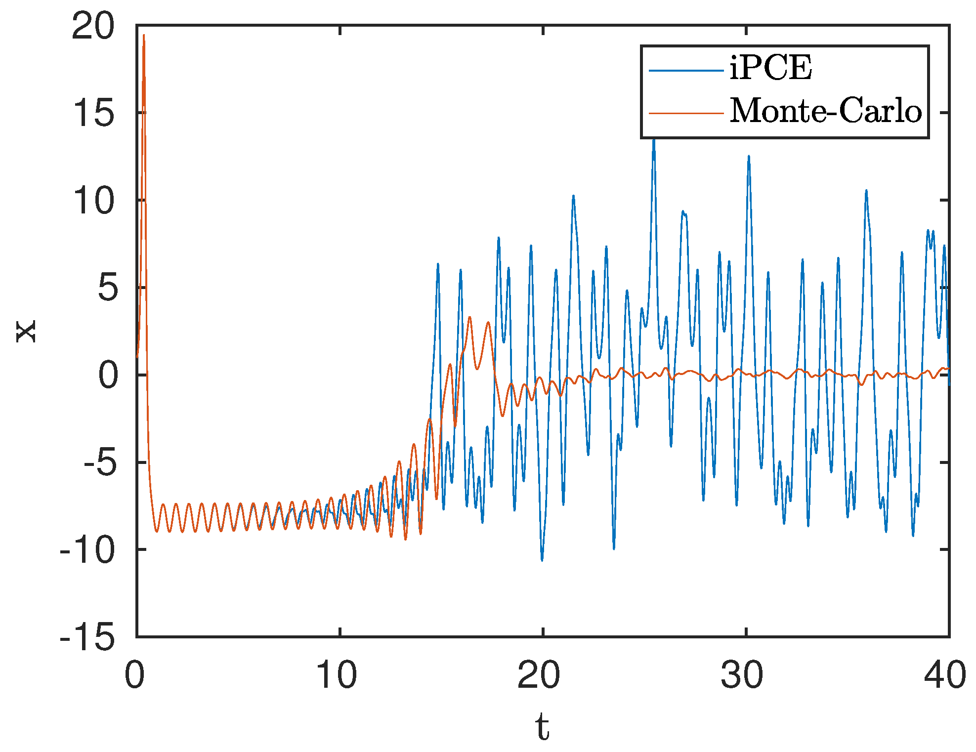
This coupled system is integrated explicitly with a variable time-step Runge Kutta and unit initial conditions. We also performed MC simulations with $N=5000$ samples over a time-frame $T=40$, which ensures the solution has become chaotic. The mean value (expectation) of the $x\left(t\right)$ coordinate of the trajectory obtained from iPCE and Monte–Carlo (MC) are compared in Figure 1.

The MC result is obtained as follows. The Lorenz equations in (25) are integrated using N sample values of $\beta$ that follow the given distribution. At each time instant t, the expectation of $x\left(t\right)$ is computed from the N available samples and plotted as a function of time. Note that the expectation tends to 0 as t increases; this is due to the symmetry of the attractor. The iPC solution, however, starts to deviate substantially from the MC at around $t=15$. Increasing the chaos order c will not alleviate this deviation; it will simply delay it at later time.

4. Non-Intrusive PC in Chaotic Systems

In the niPC, instead of applying the PCE to the state variables, we apply it directly to the QoI, as in

$${\overline{G}}_{\infty }(\xi )=\sum _{i=0}^{\infty }{\overline{G}}_{\infty }^i{\Psi }_i(\xi ),$$

(28)

and the spectral coefficients are evaluated using a quadrature approach,

$${\overline{G}}_{\infty }^i={\int }_{\mathcal{E}}{\overline{G}}_{\infty }(\xi ){\Psi }_{i}d\xi =\sum _{j=1}^{\alpha }{\omega }_j{\overline{G}}_{\infty }\left({\xi }_j\right){\Psi }_i\left({\xi }_j\right).$$

(29)

The niPC requires evaluations of the QoI at the required quadrature points ${\xi }_j$ and does not suffer from the aforementioned problem of intrusive PC. This approach is therefore suitable to chaotic systems. It is easy to apply, and most importantly, time-averaged quantities ${\overline{G}}_{\infty }\left(s\right)$ are (usually) smooth functions of the parameters s and are therefore better suited for a spectral representation. This results in a smooth convergence of the spectral expansion and allows the evaluation of the statistics with low chaos orders c, which is important for keeping the computational cost low. More applications on niPC on chaotic systems will be discussed in later sections.

The same approach can be implemented to compute the statistics of the sensitivity of ${\overline{G}}_{\infty }\left(s\right)$,

$$\frac{d{\overline{G}}_{\infty }}{ds}\approx \sum _{i=0}^q{\frac{d{\overline{G}}_{\infty }}{ds}}^i{\Psi }_i(\xi ),{\frac{d{\overline{G}}_{\infty }}{ds}}^i=\sum _{j=1}^{\alpha }{\omega }_j\frac{d{\overline{G}}_{\infty }}{ds}\left({\xi }_j\right){\Psi }_i\left({\xi }_j\right).$$

(30)

The MSS algorithm, as described in Section 2, is employed in to evaluate $\frac{d{\overline{G}}_{\infty }}{ds}\left({\xi }_j\right)$ at the quadrature points ${\xi }_j$. In the following two sections, we apply niPC for time-averaged quantities and their sensitivities on two test cases and compare the results with MC simulations.

5. Application on the Lorenz-96 Model

We apply the aforementioned methodology in the Lorenz-96 equations [25], which model the evolution of atmospheric quantities, such as vorticity or temperature at a discrete periodic lattice representing a latitude circle on earth. The model is given by the system of N equations

$$\frac{d{X}_i}{dt}=(X_{i+1}-X_{i-2})X_{i-1}-X_i+F,$$

(31)

where $i=1,\cdots ,N$. In this system, $-X_i$ is a damping term, F is an external force, and the quadratic terms resemble the advection term and conserve kinetic energy. For more details on the solution of (31) and the treatment of $X_{-1},X_0$, and $X_N$, the reader is referred to References [25,26]. This model is excellent for testing, since it is exhibits different dynamics depending on F; thus, it is ergodic, and its behavior displays similarities with turbulent fluid flows [26].

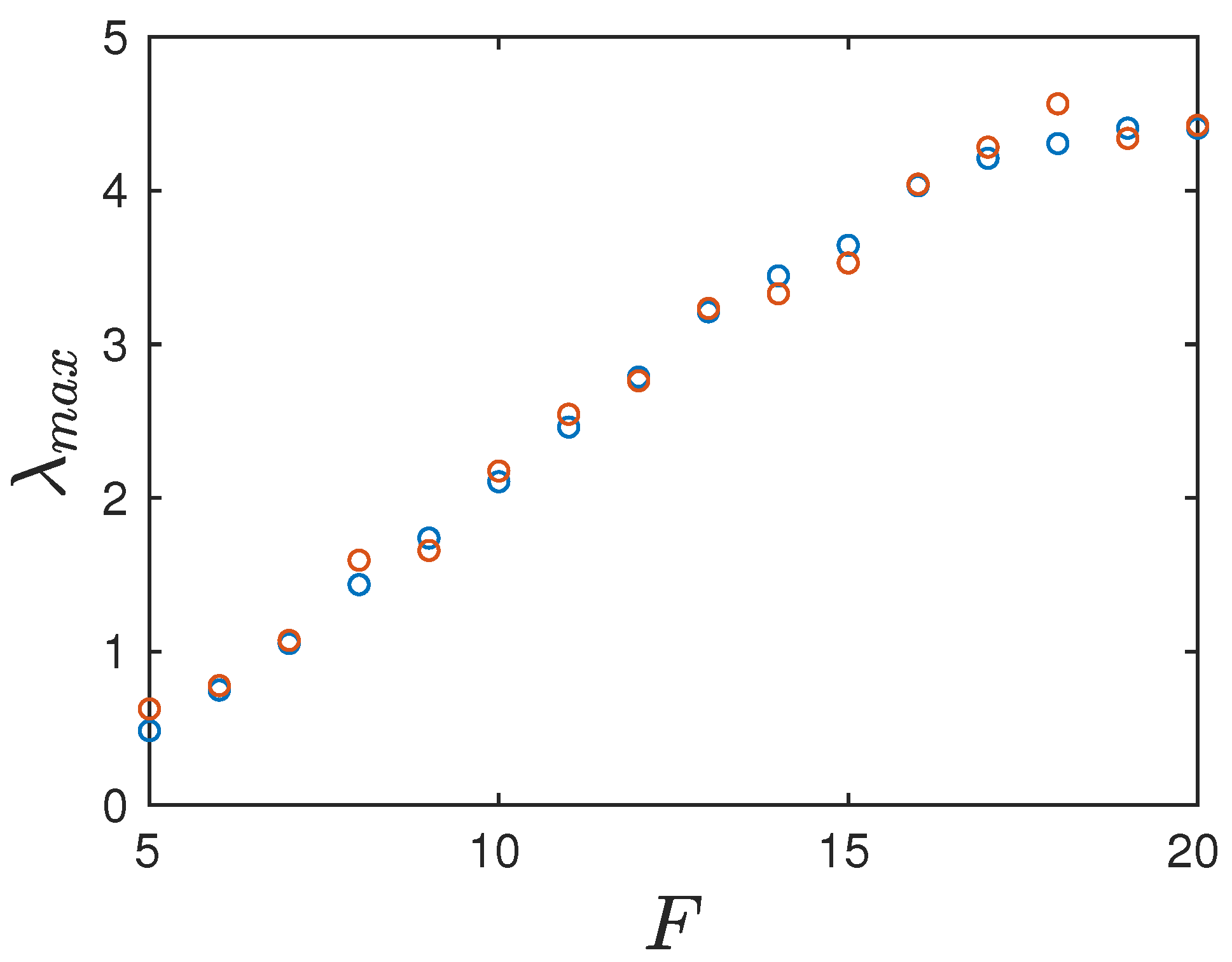
In Figure 2, we plot the maximum Lyapunov exponent of the system as a function of the forcing term F. Notice that the exponents are positive in the range of F considered, indicating that the Lorenz-96 model displays chaotic behavior. The exponents were computed using QR decomposition, as in Reference [27], and match well with the results from Reference [28].

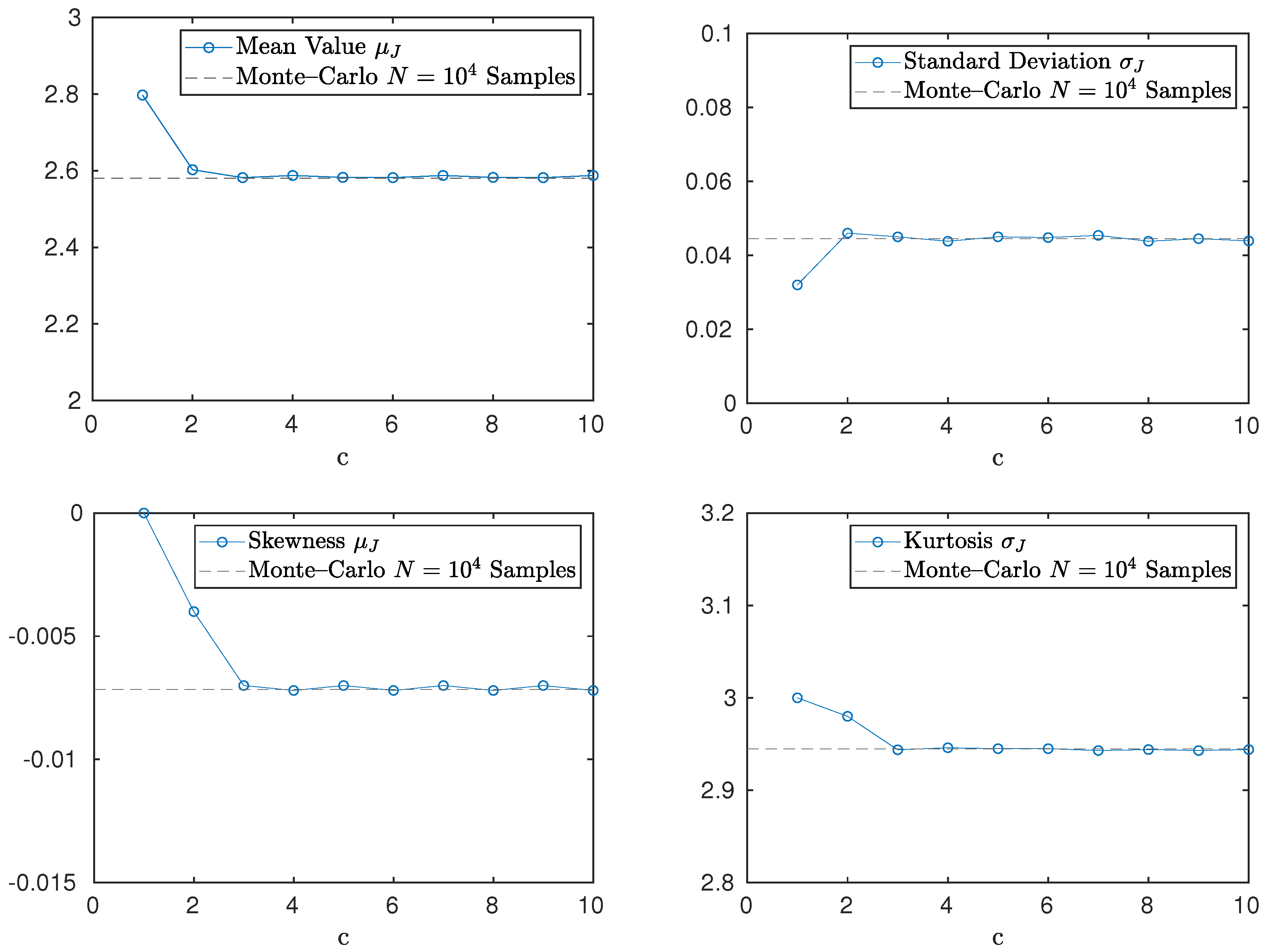
The QoI considered is the time-averaged integral of the average value of $X_i$, defined as

$$J\left(F\right)=\frac{1}{NT}\sum _{i=1}^N{\int }_0^T{X}_{i}dt.$$

(32)

Uncertainty is introduced through $F=10+0.3\xi$, where $\xi \sim \mathcal{N}\left(\mathrm{0,1}\right)$ is Gaussian. To choose an appropriate chaos order c, we perform a spectral convergence analysis for the first four moments of Equation (32), which is shown in Figure 3. Notice that, for $c=4$, all four moments stabilize to the value predicted by a Monte–Carlo simulation with $N=\mathrm{10,000}$ samples.

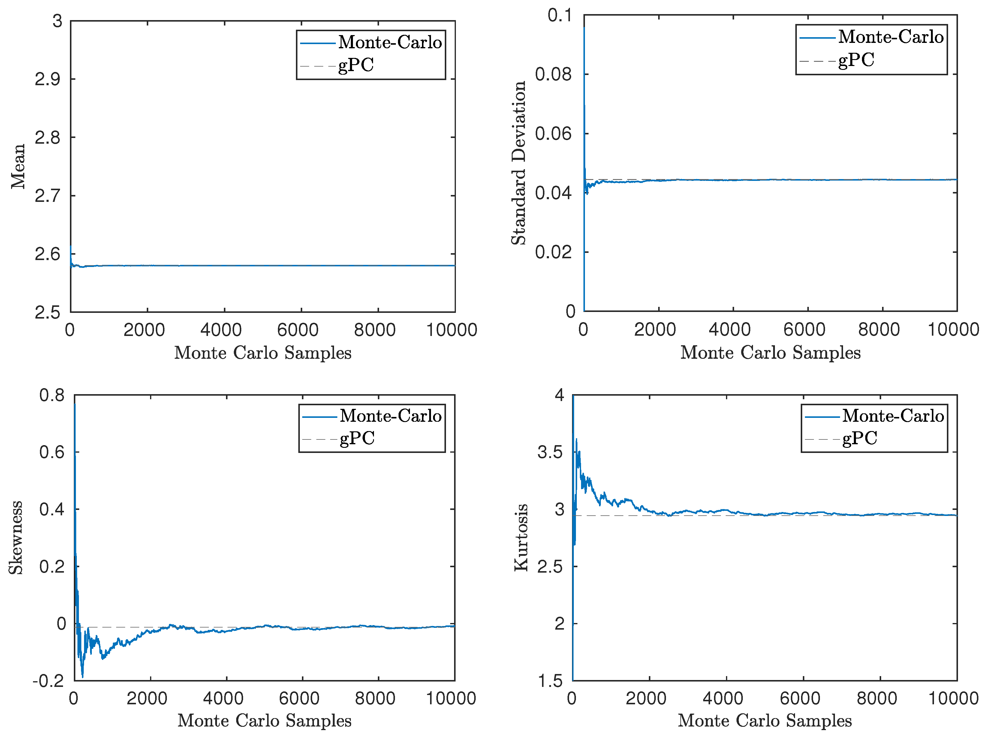
In Figure 4, we compare the first four statistical moments of Equation (32) obtained using the Monte–Carlo and gPC for $c=4$. Notice that the Monte–Carlo is in good agreement with the gPC, indicating that this approach can be a valuable method for UQ in the time averages of chaotic systems. Note that the skewness and kurtosis are close to 0 and 3, respectively, as the values for Gaussian distribution. A possible explanation is that $J\left(F\right)$ is the sum of random variables that follow the same distribution, and from the central limit theorem, it follows that the PDF of $J\left(F\right)$ is Gaussian.

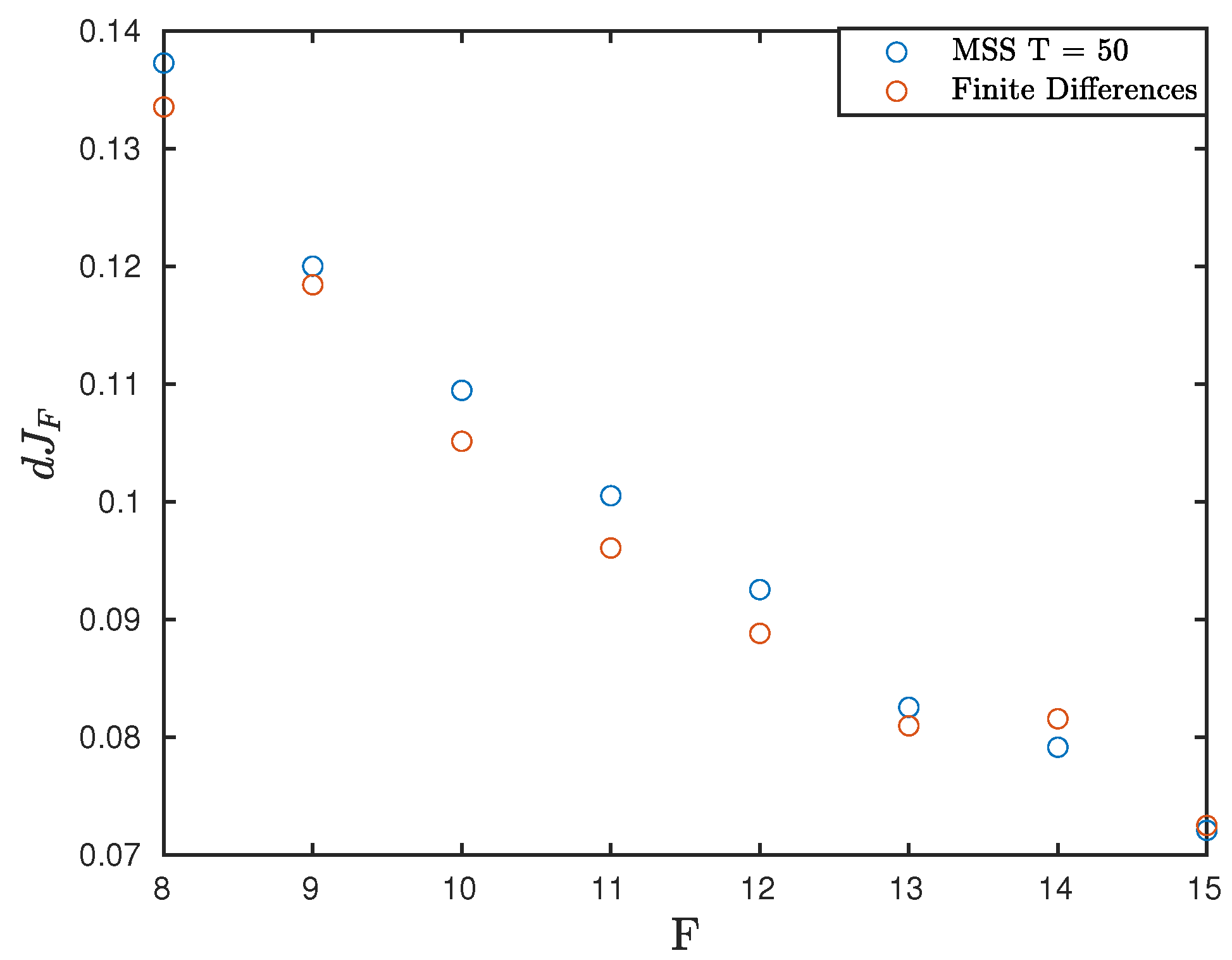
The same principle applies in the UQ of the sensitivity of QoI (32) with respect to F. This sensitivity is obtained using the MSS algorithm described in Section 2. To that end, Equation (31) is differentiated with respect to F

$$\frac{d{V}_i}{dt}=X_{i-1}{V}_{i+1}+(X_{i+1}-X_{i-2})V_{i-1}-X_{i-1}{V}_{i-2}-V_i+1-\eta \left((X_{i+1}-X_{i-2})X_{i-1}-X_i+F\right),$$

(33)

where $V_i=\frac{d{X}_i}{dF}$. Equation (33) is used as a constraint in the MSS algorithm (refer to Equation (5c)). Results can seen in Figure 5, where the sensitivity obtained from MSS is compared with FD.

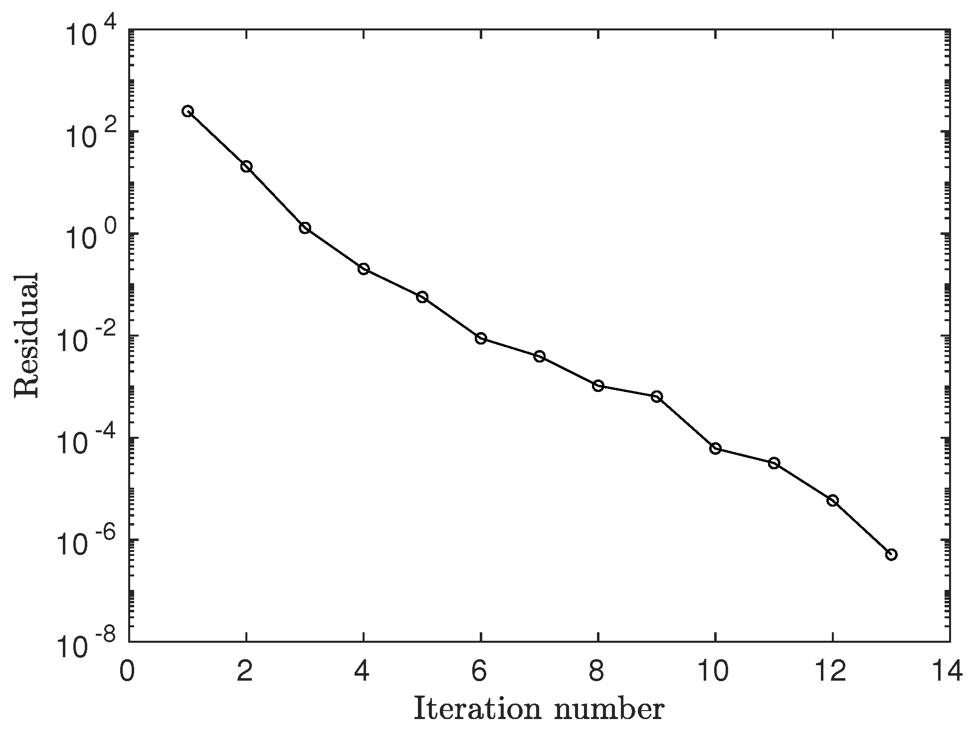
The convergence of the GMRes algorithm applied to system (14) is shown in Figure 6. The residuals are reduced by more than 8 orders of magnitude in 13 iterations, which demonstrates the effectiveness of the preconditioner.

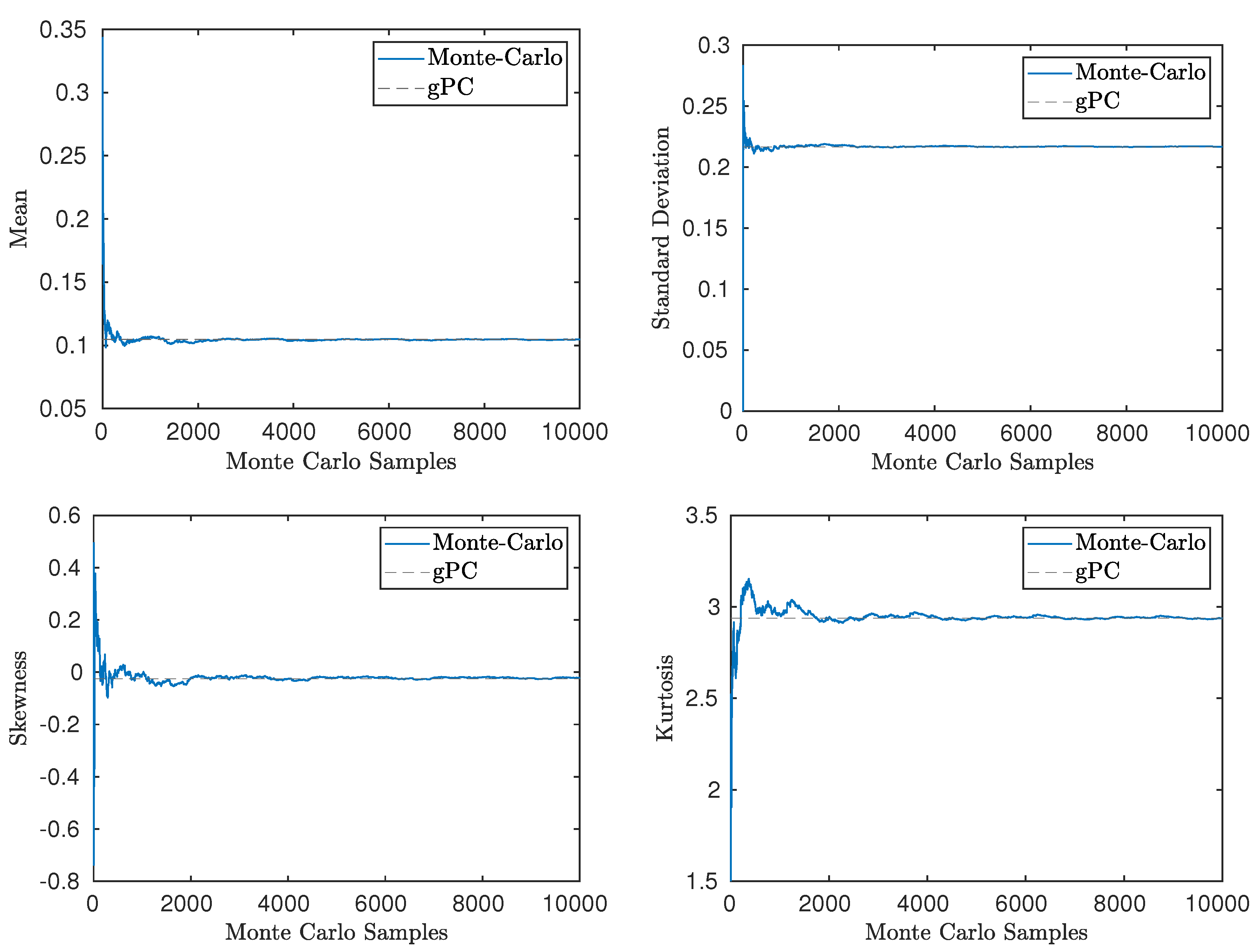
By coupling the gPC with the MSS, the statistics of the sensitivity of the QoI can be computed efficiently. In Figure 7, the first four statistical moments of $\frac{dJ}{dF}$ are computed and compared with the results from Monte–Carlo. The gPC is found to be in good agreement with the results from the Monte–Carlo simulation. Note that again the skewness and kurtosis are predicted to be close to the values of the Gaussian distribution.

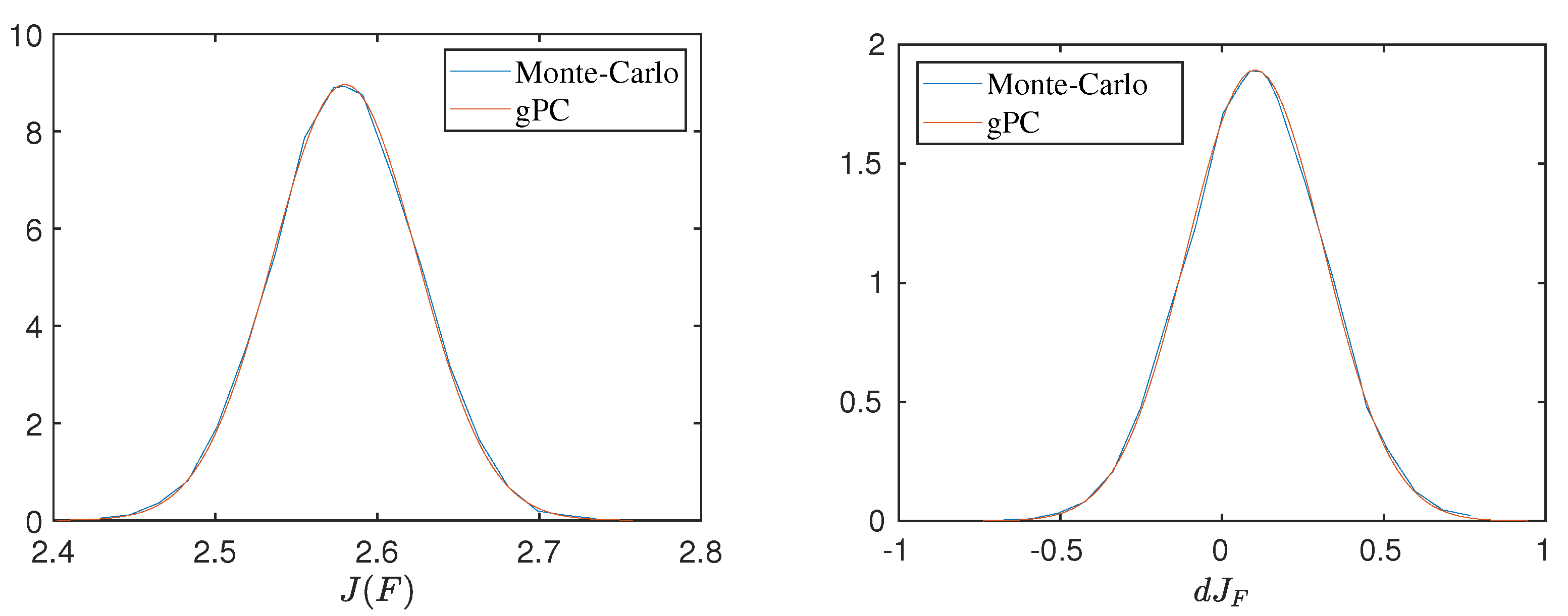
The PDF computed by the gPC coupled with the MSS can be compared with the one produced by the Monte–Carlo where the sensitivities are evaluated using FD. The PDF predicted by the gPC is computed as in Reference [14]. This is seen in Figure 8, where the PDF from the Monte–Carlo has been approximated by connecting the midpoints of the bins of its histogram. Notice that the two PDFs are in good agreement.

6. Application on the van der Pol Oscillator

The UQ methodology is now applied to the van der Pol oscillator, given by

$$\frac{d^{2}y}{d{t}^2}=-y+\beta (1-y^2)\frac{dy}{dt}.$$

(34)

This is a non–conservative oscillator, where the non-linearity is introduced through its damping coefficient. It was initially used to model limit cycle oscillations in electrical circuits, but it has been applied in other fields, as well, such us seismology and neuron modeling. The QoI is the $L_8$ norm of $\omega =\frac{dy}{dt}$, which behaves similarly to the $L_{\infty }$ norm, and provides a metric for the magnitude of the peaks of $\omega$. The objective function is written as

$${\langle J\rangle }^{\frac{1}{8}}={\left(\underset{T\to \infty }{lim}\frac{1}{T}{\int }_0^T{\omega }^{8}dt\right)}^{\frac{1}{8}}.$$

(35)

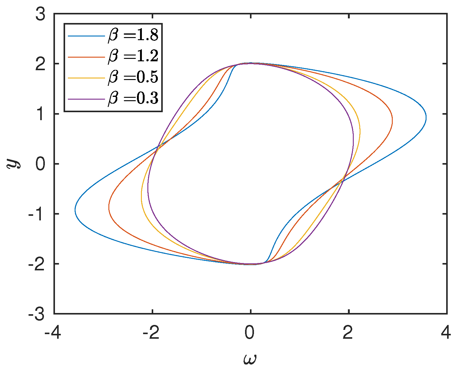
Equation (34) is converted into a set of two, coupled ODEs [29] and integrated from an initial condition at $t=-50$ until $t=0$, which ensures that the state variable $u=[y,\omega ]$ has reached the attractor. Further integration then follows from 0 to T to obtain the reference trajectory. The attractor of the state u is seen in Figure 9.

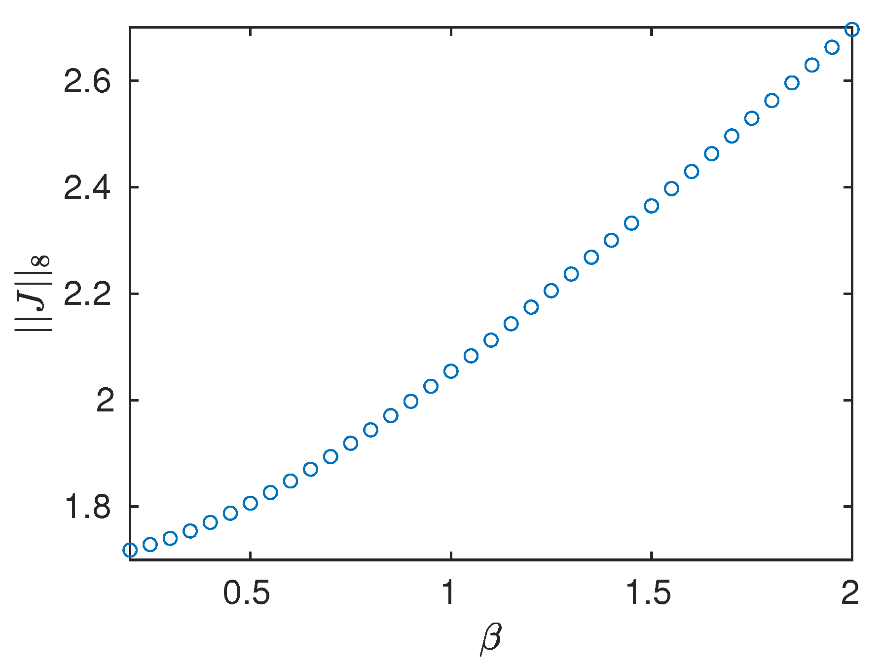
Integrating Equation (34) forward in time is computationally inexpensive; therefore, we can easily compute the variation QoI with $\beta$ for a wide range of values. This is shown in Figure 10; ${\langle J\rangle }^{\frac{1}{8}}$ increases in magnitude as $\beta$ increases.

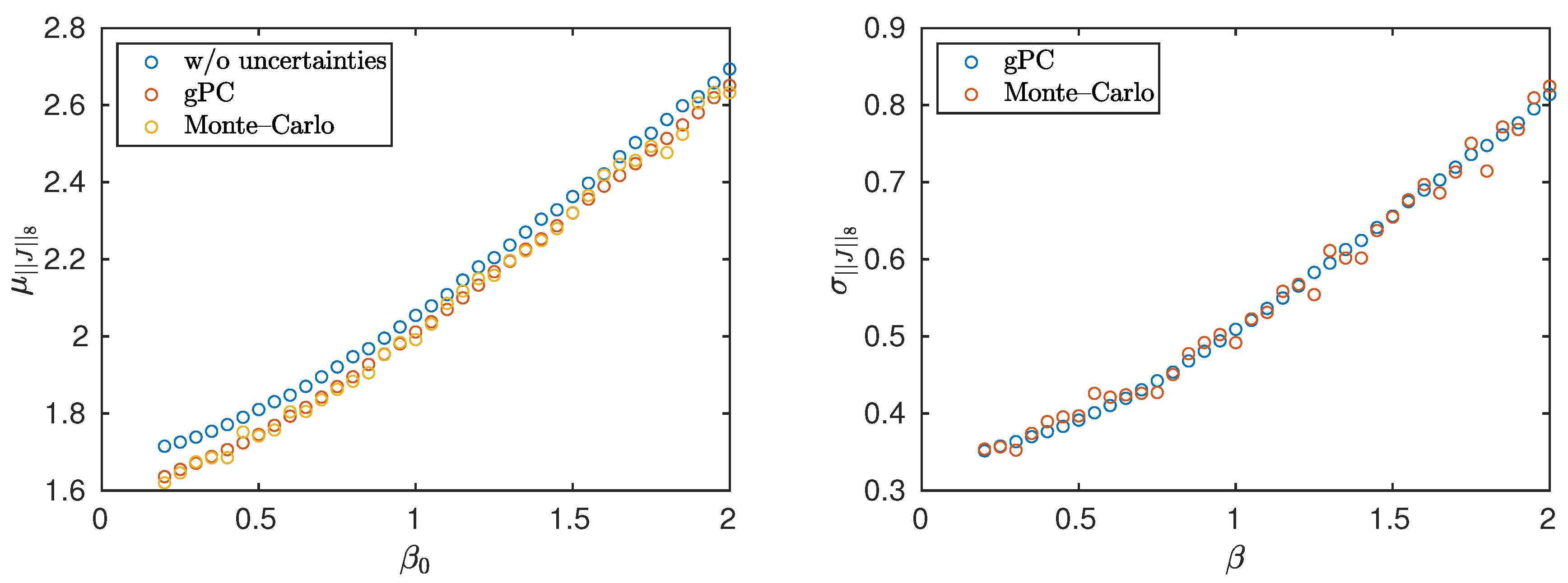
The variation is smooth; therefore, it is expected that the gPC can be used to efficiently compute the statistics of ${\langle J\rangle }^{\frac{1}{8}}$. This is seen in Figure 11, where a comparison is made between the gPC and the MC. Note that the selection of the number of samples for the MC and the chaos order c was made through a spectral convergence study for the gPC and through a sample convergence study for the MC, similarly to the Lorenz-96 case. Uncertainty is introduced through $\beta ={\beta }_0+{\beta }_1\xi$, where ${\beta }_0$ varies in $\left[\mathrm{0.2,2}\right]$ with a step of $\delta b=0.05$, $\xi \sim \mathcal{N}(0,1)$ is Gaussian, and ${\beta }_1=0.5{\beta }_0$. Notice that the two methods are again in good agreement. It is worth mentioning that there is a slight deviation with respect to the value obtained in the absence of uncertainties (blue circles). This deviation, arising from a deterministic approach to chaotic systems, is important and results in overestimation of the QoI if uncertainties are not taken into account.

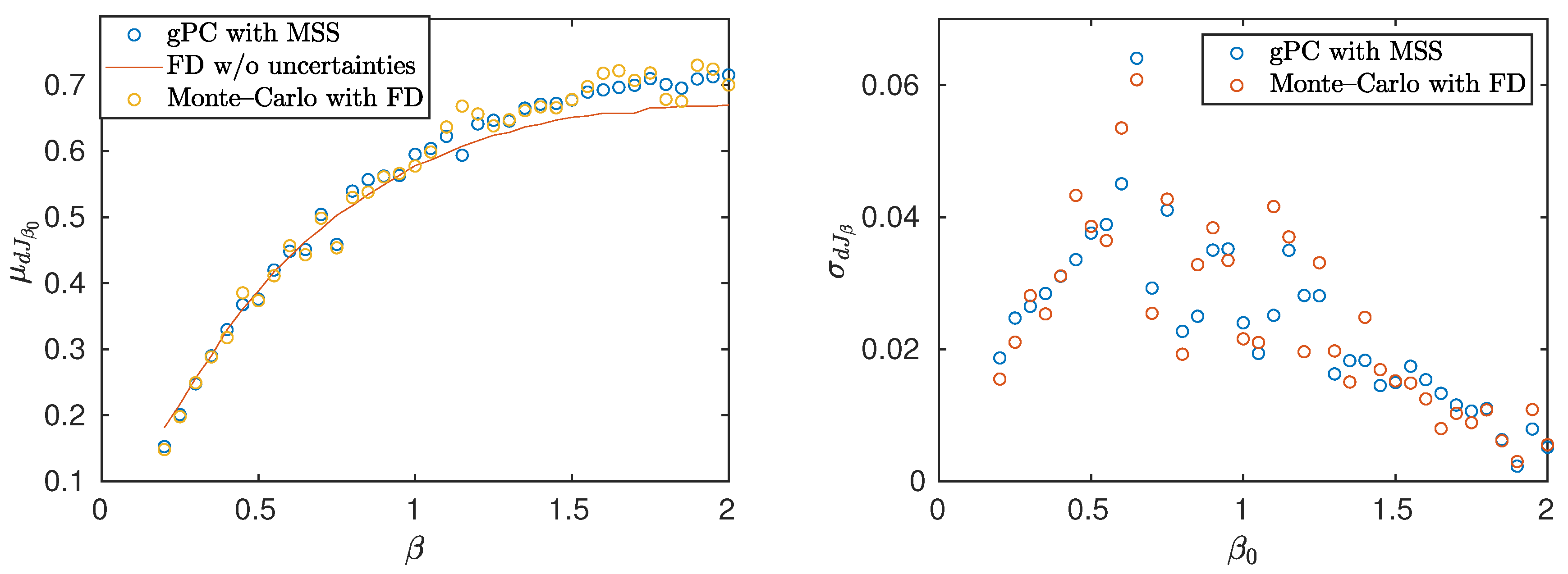
The smooth behavior shown in Figure 10 implies also a smooth variation of the sensitivity $d{\langle J\rangle }^{\frac{1}{8}}/d\beta$ with respect to $\beta$. This is verified in Figure 12 (left), where the mean value is computed with FD for a time-length of $T=1000$. In the same figure, a comparison is made between the gPC coupled with MSS, and the Monte–Carlo for $N=5000$ samples. Uncertainty conditions are the same as in Figure 11.

Notice that the gPC is in good agreement with the MC. A small deviation, similar to that found in Figure 11, is also observed in the sensitivities. Here, the deviation is found for even smaller uncertainties, which indicates an even stronger influence of the non-linearity present in the design space of Equation (35).

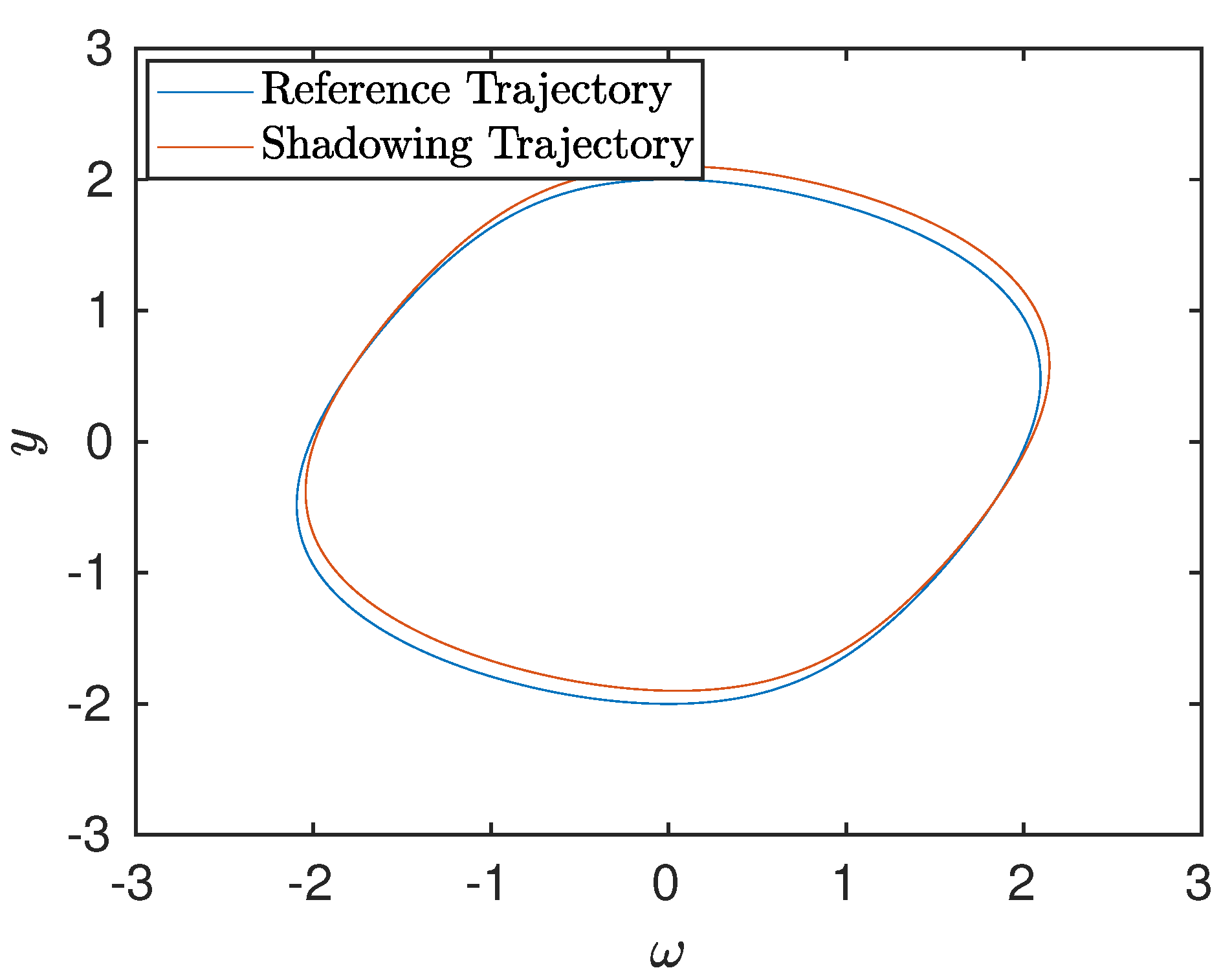
In Figure 13, we plot the reference trajectory and its shadowing counterpart, in phase space. The difference between the two trajectories is exaggerated by two orders of magnitude so that a visual can be produced. Notice that the two trajectories remain close, i.e., shadow, each other in phase space. It is exactly this property that allows us to compute reliable sensitivities in chaotic systems.

7. Discussion

The results from Section 5 and Section 6 indicate that the non-intrusive gPC is a valid method for quantifying uncertainties of time-averages and their sensitivities with respect to system parameters in chaotic systems. The gPC is an established method in propagating and evaluating uncertainties, yet the accuracy of the intrusive version deteriorates when applied to general unsteady (let alone chaotic) systems. This was demonstrated in the Lorenz attractor, where it was shown that the statistics of the trajectory cannot be captured correctly with an iPC approach. Approaches where the orthonormal basis is recalculated and the spectral order of the expansion is increased have appeared in the literature [30,31]; however, these approaches have high computational cost and increased complexity.

Non-intrusive approaches, on the other hand, do not suffer from the aforementioned problem. This is demonstrated on the Lorenz-96 system and the van der Pol oscillator, where the statistics of the time-averages are computed accurately for a low spectral chaos order c, the results being in good agreement with the MC. The convergence of the gPC for low c is due to the fact that the time-averages display smooth variation to system parameters, as well as due to ergodicity are independent of the initial conditions used. The computational cost of this method scales with the number of stochastic parameters. In such high-dimensional cases, correlations may exist between the uncertain parameters. These issues are dealt with in the gPC literature with the use of sparse grids, data–driven techniques, or variational approaches, [1,3,32].

Regarding the sensitivities, to properly evaluate their statistics, the gPC is coupled with the MSS algorithm, which can accurately compute the sensitivities of time-averages, even for a large number of uncertain parameters. The MSS algorithm is formulated in such a way to allow for the non-intrusive nature of the niPC to be preserved and for already developed software conducting the sensitivity analysis of the system to be employed. This coupling introduces a basic algorithmic framework for conducting UQ in chaotic systems and can exist as a basis for developing an approach to robust design in the presence of chaos.