Uncertainty Propagation through a Point Model for Steady-State Two-Phase Pipe Flow

Abstract

Uncertainty propagation is used to quantify the uncertainty in model predictions in the presence of uncertain input variables. In this study, we analyze a steady-state point-model for two-phase gas-liquid flow. We present prediction intervals for holdup and pressure drop that are obtained from knowledge of the measurement error in the variables provided to the model. The analysis also uncovers which variables the predictions are most sensitive to. Sensitivity indices and prediction intervals are calculated by two different methods, Monte Carlo and polynomial chaos. The methods give similar prediction intervals, and they agree that the predictions are most sensitive to the pipe diameter and the liquid viscosity. However, the Monte Carlo simulations require fewer model evaluations and less computational time. The model predictions are also compared to experiments while accounting for uncertainty, and the holdup predictions are accurate, but there is bias in the pressure drop estimates.

1. Introduction

Multiphase flow models are used in a range of applications, such as petroleum transport, nuclear energy and biomechanics. Accuracy in the model output is required to ensure the models to be useful decision support tools. Consequently, there is a rapid development in methods for quantifying the uncertainty in these models.

Lee and Chen [1] compared several types of uncertainty propagation methods, including Monte Carlo methods (MC), polynomial chaos expansions (PC), full-factorial numerical integration (FFNI) and univariate dimension reduction (UDR). They explain the relative strengths of each method, and one conclusion is that PC is most viable in comparison to FFNI and UDR when input distributions are normal but output distributions are not. This is the situation in our analysis. Later, Cremaschi et al. [2] discussed applications of the methods discussed in Lee and Chen [1] to multiphase flows. Furthermore, they asked in the short-term that vendors of multiphase simulators implement tools for propagating uncertainty and yield sensitivities and prediction intervals. It was also requested that the simulators incorporate uncertainty in closure laws and that researchers accompany experimental data with uncertainty estimates. In the long term, Cremaschi et al. [2] recommended producing scale-up data to improve extrapolation in multiphase models. A case study is presented in Holm et al. [3,4], where they demonstrated how uncertainty propagation may be used for flow assurance on the Shtokman gas and condensate field. Their analysis included pressure drop and liquid holdup predictions using a one-dimensional model in the software OLGA. They determined probability distributions for a selection of input variables and closure laws and they propagated these uncertainties through the multiflow model using a Monte Carlo method. The result is the 10th, 50th, and 90th output percentiles for pressure drop and liquid holdup predictions and measures of sensitivity to the input variables. Hoyer et al. [5] used Monte Carlo simulations with OLGA in order to identify influential variables and closure laws in several groups of data with different flow conditions. They are only able to construct satisfactory probability distributions for each closure law when using a group of data where the closure law is significant.

Klavetter et al. [6] modeled liquid holdup and pressure drop in two-phase pipe flow using the TUFFP Unified Model for two-phase flow. They assumed an uncertainty range for each input variable and compared perturbation, Taylor series approximations and Monte Carlo methods for uncertainty propagation. They concluded that Taylor series approximations overestimate the output uncertainty while the other methods perform well. Keinath et al. [7] also demonstrated the importance of selecting an appropriate framework when handling uncertainty in multiphase modeling and highlighted the value of quantitative information about the input uncertainty distributions for decision making.

Just recently, in Liu et al. [8], a Gaussian process and principal component analysis were applied to a complex two-phase flow model in order to explore the uncertainty and reduce the complexity of the model. Picchi and Poesio [9] considered a one-dimensional model for two-phase pipe flow. Known distributions for input variables are propagated through the model using Monte Carlo methods to obtain first-order and total sensitivity indices as well as output distributions. In the thesis of Klinkert [10], a similar method was applied to the point model Shell Flow Correlations and the one-dimensional model PIPESIM by Schlumberger. Polynomial chaos expansions were also applied, and both analyses were implemented in the open-source software UQLab [11].

In this work, we compare uncertainty estimates obtained by Monte Carlo simulations with those of polynomial chaos for the two-phase point model presented in Smith et al. [12]. The analyses include quantifying the uncertainty in the model output and estimating the sensitivity to each input variable. Furthermore, we explicitly compare the computational cost of MC to that of PC. These comparisons are important for practical use but uncommon in the literature.

The flow model predicts average holdup and pressure drop based on mass rates, viscosities, densities, pipe diameter, hydraulic roughness, surface tension and pipe inclination. The uncertainty framework provides prediction intervals and the sensitivity to each input variable. We use 240 experiments of stratified flow or slug flow from the SINTEF Multiphase Flow Laboratory as reference. These experiments were also studied in Smith et al. [12]. The comparison of prediction intervals to measurement intervals provides high-quality information about any bias in the physical model because the uncertainty is handled in a careful manner.

Section 2 contains details on the flow model and the uncertainty quantification framework. The results are presented in Section 3 and discussed in Section 4.

2. Materials and Methods

2.1. Flow Model

We analyzed the model developed in Smith et al. [12], only with a small change to turbulent interpolation. This section briefly outlines their model, which considers two-phase flow in a circular pipe and predicts liquid holdup H and pressure drop $-p^{\prime }=-\partial p/\partial x$ in the longitudinal direction x. The model predictions are based on ten measured input variables listed in

Table 1. Input to the flow model. The index p refers to phase, where g is gas and l is liquid.

Symbol	Description	Unit
${\dot{m}}_p$	Mass rate	kg/s
${\mu }_p$	Viscosity	Pa s
${\rho }_p$	Density	Pa s
D	Pipe diameter	m
$\epsilon$	Hydraulic roughness	m
$\sigma$	Surface tension	N/m
$\theta$	Pipe inclination	rad

. In contrast to the presented approach, system identification with a backward elimination method [13,14], forward selection [15] or stepwise regression [16] can be used for the same purpose. This would raise the model quality, but also increase the experiment cost and computational time significantly, and is not applied in this paper.

The flow is categorized as either stratified, bubbly or slug flow. All cases are covered by a unit-cell model, as introduced in Dukler and Hubbard [17]. The holdup is the weighted average

$$H=s{H}_{\mathrm{s}}+(1-s)H_{\mathrm{l}},$$

(1)

where s is slug fraction, $H_{\mathrm{s}}$ is the slug zone holdup and $H_{\mathrm{l}}$ is the bubble zone holdup. Slug flow is illustrated in Figure 1. The model allows for gas bubbles in the slug. Note that $s\le 0$ is stratified flow and $s\ge 1$ is bubbly flow, and s is then limited to 0 and 1, respectively, in the weighting.

The estimation procedure consists of two main steps, deciding the flow regime and computing the holdup conditional on that regime. In general, we need the conditional holdups in order to decide on the regime.

2.1.1. Slug Zone

The slug zone holdup is computed first. We apply Gregory et al. [18] for low liquid viscosities and Kora et al. [19] for higher ones. It is convenient to introduce average superficial velocities, defined as

$$U_p=\frac{4{\dot{m}}_p}{\pi D^2{\rho }_p},$$

(2)

where the index p refers to phase, with g for gas and l for liquid. The slug zone holdup is

$$H_{\mathrm{s}}=\{\begin{array}{cc}\frac{1}{{1+0.05\left\{U\mathrm{m}\right\}}^{1.39}},\hfill & \hspace{1em}{\mu }_{\mathrm{l}}<0.02\hfill \\ 1,\hfill & \hspace{1em}{\mu }_{\mathrm{l}}\ge 0.02,k\le 0.15\hfill \\ 1.012·e^{-0.085k},\hfill & \hspace{1em}{\mu }_{\mathrm{l}}\ge 0.02,0.15<k<1.5\hfill \\ 0.9473·e^{-0.041k},\hfill & \hspace{1em}{\mu }_{\mathrm{l}}\ge 0.02,k\ge 0.15\hfill \end{array}$$

(3)

where $k=U_{\mathrm{m}}^{1.2}{D}^{-0.9}{g}^{-0.7}{\mu }_{\mathrm{l}}^{0.2}{\rho }_{\mathrm{l}}^{0.5}{({\rho }_{\mathrm{l}}-{\rho }_{\mathrm{g}})}^{-0.7}$ and $U_{\mathrm{m}}=U_{\mathrm{g}}+U_{\mathrm{l}}$ is the mix velocity with the numerical value denoted as {Um}. Using the slug zone holdup, we can easily check for bubbly flow. The holdup for bubbly flow is

$$H=\frac{U_{\mathrm{l}}}{U_{\mathrm{m}}}\mathrm{if}{U}_{\mathrm{l}}>U_{\mathrm{m}}{H}_{\mathrm{s}}.$$

(4)

The requirement corresponds to a slug fraction greater than 1. In order to find the average holdup in slug flow, we need the bubble nose velocity, which is also empirical. Smith et al. [12] used a modified version of the function proposed in Bendiksen [20]. The bubble nose velocity is assumed linear in the mix velocity with an intercept determined by the experiments conveyed in Jeyachandra et al. [21]. The slope $C_0$ is interpolated from a laminar value and a turbulent value, as proposed in Nuland [22], with some additional restrictions. Details are given in Section 2.1.5. The laminar and turbulent values are

$$\begin{array}{}\hfill \mathrm{(5a)}& C_0^{\mathrm{l}}=2\hfill \hfill \mathrm{(5b)}& C_0^{\mathrm{t}}=1+2.5871\sqrt{f_{\mathrm{s}}^{\mathrm{t}}}+1.4874f_{\mathrm{s}}^{\mathrm{t}},\hfill \end{array}$$

where $f_{\mathrm{s}}^{\mathrm{t}}$ is the slug friction factor defined later. The turbulent value is as reported in Hinze [23]. Using this approach, the bubble nose velocity is

$$\begin{array}{c}\hfill u_{\mathrm{b}}=U_0(F+0.351tan\theta )+U_{\mathrm{m}}·max\left(C_0+0.15{sin}^2\theta ,1.05+0.15{sin}^2\theta ,1.2-\frac{U_{0}F}{U_{\mathrm{m}}}\right),\end{array}$$

(6)

where $U_0=cos\theta \sqrt{Dg({\rho }_{\mathrm{l}}-{\rho }_{\mathrm{g}})/{\rho }_{\mathrm{l}}}$ and $F=0.53exp(-13.7D^{-0.89}{\left(g{\rho }_{\mathrm{l}}\right)}^{-0.33}{({\rho }_{\mathrm{l}}-{\rho }_{\mathrm{g}})}^{-0.23}{\mu }_{\mathrm{l}}^{0.46}{\sigma }^{0.1})$.

2.1.2. Bubble Zone

Let $H_{\mathrm{g}}=1-H_{\mathrm{l}}$ be the gas fraction in the bubble zone. The liquid holdup in the bubble zone is the solution to the momentum balance for both phases, that is $H_{\mathrm{l}}$ such that

$$\begin{array}{c}\hfill {\rho }_{\mathrm{g}}{f}_{\mathrm{g}}{S}_{\mathrm{g}}{u}_{\mathrm{g}}^2{H}_{\mathrm{g}}^3-{\rho }_{\mathrm{l}}{f}_{\mathrm{l}}{S}_{\mathrm{l}}{u}_{\mathrm{l}}^2{H}_{\mathrm{l}}^3+{\rho }_{\mathrm{g}}{f}_{\mathrm{i}}{S}_{\mathrm{i}}(u_{\mathrm{l}}{H}_{\mathrm{l}}-u_{\mathrm{g}}{H}_{\mathrm{g}})|u_{\mathrm{l}}{H}_{\mathrm{l}}-u_{\mathrm{g}}{H}_{\mathrm{g}}|+({\rho }_{\mathrm{l}}-{\rho }_{\mathrm{g}})\frac{\pi }{4}{D}^2{H}_{\mathrm{g}}^3{H}_{\mathrm{l}}^{3}gsin\theta =0,\end{array}$$

(7)

where the perimeters $S_p$ and $S_{\mathrm{i}}$ are defined in Figure 1, and the friction factors $f_p$ and $f_{\mathrm{i}}$ are defined below. The superficial velocities $u_p$ must be chosen according to the flow regime. The superficial velocities equal the average superficial velocities in Equation (2) for stratified flow, while they are functions of the bubble zone holdup for slug flow, namely

$$\begin{array}{}\hfill \mathrm{(8a)}& \mathrm{Stratified}\mathrm{flow}\hfill & :& u_p=U_p\hfill \mathrm{(8b)}& \hfill \mathrm{Slug}\mathrm{flow}& :& \left\{\begin{array}{c}\begin{array}{c}\hfill u_{\mathrm{g}}=U_{\mathrm{g}}+\Delta \\ \hfill u_{\mathrm{l}}=U_{\mathrm{l}}-\Delta .\end{array}\hfill \end{array}\right.\hfill \end{array}$$

where $\Delta =(H_{\mathrm{s}}-H_{\mathrm{l}})u_{\mathrm{b}}+(1-H_{\mathrm{s}})U_{\mathrm{l}}-H_{\mathrm{s}}{U}_{\mathrm{g}}$. Furthermore, the interface friction factor is a modified version of the expression proposed in Andreussi and Persen [24] and is given by

$$\begin{array}{c}\hfill f_{\mathrm{i}}=f_{\mathrm{i}0}\left(1+10h{\left(\frac{2u_{\mathrm{g}}}{H_{\mathrm{g}}D}\sqrt{\frac{S_{\mathrm{i}}{\rho }_{\mathrm{g}}}{\pi H_{\mathrm{g}}g({\rho }_{\mathrm{l}}-{\rho }_{\mathrm{g}})cos\theta }}-0.36\right)}^{0.67}\right),\end{array}$$

(9)

where h is the line fraction approximated by

$$\begin{array}{c}\hfill h=1-cos\left(\frac{1}{3}+{\left(\frac{3\pi }{2}\right)}^{\frac{1}{3}}+\left(\pi -\frac{2}{3}\right)H_{\mathrm{l}}+H_{\mathrm{l}}^{\frac{1}{3}}+H_{\mathrm{g}}^{\frac{1}{3}}\right)\end{array}$$

(10)

and we impose a minimum of $f_{\mathrm{i}0}=f_{\mathrm{g}}(\epsilon =0)$. The friction factors $f_{\mathrm{i}0}$, $f_{\mathrm{g}}$, $f_{\mathrm{l}}$ and $f_{\mathrm{s}}$ are interpolated from laminar and turbulent values, as described in Section 2.1.5. We use the Hagen-Poiseuille and Haaland formulas found in White [25] given as

$$\begin{array}{}\hfill \mathrm{(11a)}& f_p^{\mathrm{l}}=16\mathrm{R}{p}^{-1}\hfill \hfill \mathrm{(11b)}& f_p^{\mathrm{t}}=0.07716·{log}_{10}^{-2}\left(6.9\mathrm{R}\mathrm{e}{p}^{-1}+0.234{\left(\frac{\epsilon }{D}\right)}^{1.11}\right),\hfill \end{array}$$

where

$$\mathrm{R}\mathrm{e}{p}^{-1}=\{\begin{array}{cc}\hfill {\displaystyle \frac{{\mu }_{\mathrm{g}}(S_{\mathrm{g}}+S_{\mathrm{i}})}{\pi D^2{\rho }_{\mathrm{g}}\left|u_{\mathrm{g}}\right|}},& p=\mathrm{g}\\ {\displaystyle \frac{{\mu }_{\mathrm{l}}{S}_{\mathrm{l}}}{\pi D^2{\rho }_{\mathrm{l}}\left|u_{\mathrm{l}}\right|}},& p=\mathrm{l}\\ {\displaystyle \frac{{\mu }_{\mathrm{l}}}{D{\rho }_{\mathrm{m}}^{\mathrm{s}}{U}_{\mathrm{m}}}},& p=\mathrm{s}\end{array}$$

(12)

and ${\rho }_{\mathrm{m}}^{{}_p}=(1-H_p){\rho }_{\mathrm{g}}+H_p{\rho }_{\mathrm{l}}$ is the mix density where p is l or s for bubble zone or slug zone, respectively. The comparative study in Brkić and Praks [26] suggests a more accurate and computationally efficient approximation than Equation (10b) for the Colebrook turbulent friction factor. However, model tuning is not the main objective for this work. Instead, we use the Haaland approximation to allow for comparison to Smith et al. [12]. The friction factor is a small contributor to the computational cost of the point model. Thus, it is not essential to find the most efficient approximation.

2.1.3. Slug Fraction

The fraction of the unit-cell covered by the slug is called the slug fraction, and it may be computed as

$$\begin{array}{c}\hfill s=1+\frac{(1-H_{\mathrm{s}})U_{\mathrm{l}}-H_{\mathrm{s}}{U}_{\mathrm{g}}}{(H_{\mathrm{s}}-H_{\mathrm{l}})u_{\mathrm{b}}}.\end{array}$$

(13)

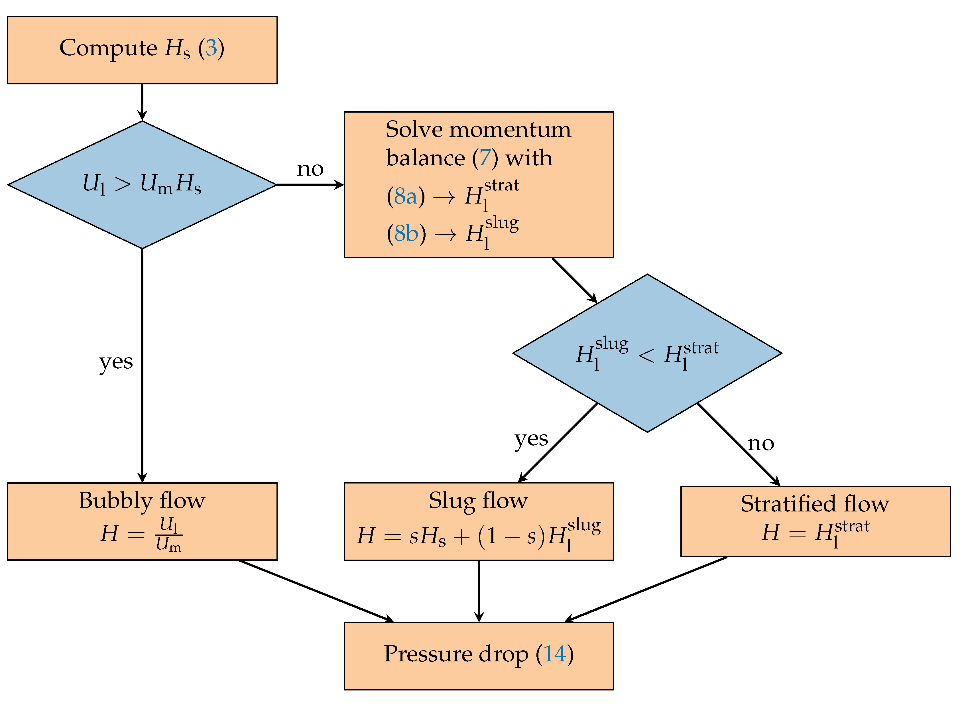
Figure 2 shows a flowchart of the steady-state point model solution procedure. The first step is to compute the slug zone holdup from (3). Next, we determine the correct flow regime and average liquid holdup. Finally, the pressure drop is computed.

2.1.4. Pressure Gradient

The pressure gradient is the weighted average

$$\begin{array}{c}\hfill p^{\prime }=s{p}_{\mathrm{s}}^{\prime }+(1-s)p_{\mathrm{l}}^{\prime },\end{array}$$

(14)

where the slug zone and bubble zone pressure gradients are

$$\begin{array}{}\hfill \mathrm{(15a)}& p_{\mathrm{s}}^{\prime }=-\frac{2}{D}{\rho }_{\mathrm{m}}^{\mathrm{s}}{f}_{\mathrm{s}}{U}_{\mathrm{m}}^2-{\rho }_{\mathrm{m}}^{\mathrm{s}}gsin\theta \hfill \hfill \mathrm{(15b)}& p_{\mathrm{l}}^{\prime }=-\frac{2}{\pi D^2}\left(\frac{{\rho }_{\mathrm{g}}{f}_{\mathrm{g}}{S}_{\mathrm{g}}{u}_{\mathrm{g}}^2}{H_{\mathrm{g}}^2}+\frac{{\rho }_{\mathrm{l}}{f}_{\mathrm{l}}{S}_{\mathrm{l}}{u}_{\mathrm{l}}^2}{H_{\mathrm{l}}^2}\right)-{\rho }_{\mathrm{m}}^{\mathrm{l}}gsin\theta ,\hfill \end{array}$$

where $H_{\mathrm{g}}$ and $H_{\mathrm{l}}$ is the solution to Equation (6).

2.1.5. Interpolation by Reynolds Number

Several dimensionless numbers g in the model are computed as $g_{\mathrm{l}}$ for laminar cases and as $g_{\mathrm{t}}$ for turbulent cases. By interpolation, we ensure continuity in g(Rep), also in the transition from laminar to turbulent. Let the laminar region be Rep < a, the transitional region be a < Rep < b and the turbulent region be b < Rep. A natural interpolation is

$$\begin{array}{}\hfill \mathrm{(16a)}& g\left(\mathrm{R}{\mathrm{e}}_p\right)\hfill & =& w{g}_{\mathrm{l}}+(1-w)g_{\mathrm{t}}\hfill \mathrm{(16b)}& \hfill w& =& \frac{b-\mathrm{R}{\mathrm{e}}_p}{b-a}.\hfill \end{array}$$

We chose $a=1700$ and $b=4000$ for the friction factors in Equation (11) except for $f_{\mathrm{s}}$. For $f_{\mathrm{s}}$ and the slopes in Equation (5), we use $b=3000$ and a such that $f_{\mathrm{l}}(\mathrm{R}\mathrm{e}=a)=f_{\mathrm{t}}(\mathrm{R}\mathrm{e}=a)$.

However, using weights w will not produce a smooth function g. In fact, the derivative of g with respect to Re is discontinuous at a and b. This far, we have outlined the model given by Smith et al. [12], but we suggest replacing the weights by ${\omega }^{\prime }={\sin }^2(\pi \omega /2)$. These weights provide continuity in the derivative of g. The change is demonstrated in Figure 3 The histograms in the left panel show the distribution of holdup estimates obtained by perturbation of a certain set of inputs with a Reynolds number close to 3000. Blue gives the holdup estimates using the original model with weights w, while orange gives the estimates obtained using the new weights ${\omega }^{\prime }$. The right panel shows C₀(Re) in the transition from laminar to turbulent Reynolds numbers. We prefer the modified model because the distribution with small changes in input is more straightened out. However, the distribution of pressure drop is nearly unchanged.

2.2. Uncertainty Quantification

Section 2.1 describes how we can predict holdup or pressure drop from measured inputs. In this section, we explain how to compute the effect of measurement error in input variables on the predictions. First, we will discuss the measurement error in each input and output. The uncertainties are attained from

Table 2. Uncertainty in the model variables given as one standard deviation.

(a) Input
Variable	Unit	Uncertainty
${\dot{m}}_{\mathrm{g}}$	kg/s	${\dot{m}}_{\mathrm{g}}·0.4\%$
${\dot{m}}_{\mathrm{l}}$	kg/s	${\dot{m}}_{\mathrm{l}}·0.05\%$
${\mu }_{\mathrm{g}}$	Pa s	${\mu }_{\mathrm{g}}·2\%$
${\mu }_{\mathrm{l}}$	Pa s	${\mu }_{\mathrm{l}}·3\%$
${\rho }_{\mathrm{g}}$	kg/m3	0.2 kg/m3
${\rho }_{\mathrm{l}}$	kg/m3	1 kg/m3
D	m	$D·1\%$
$\epsilon$	m	$1·{10}^{-6}m$
$\sigma$	N/m	$\sigma ·30\%$
$\theta$	$\mathrm{rad}$	$2·{10}^{-4}\mathrm{rad}$
(b) Output
Variable	Unit	Uncertainty
H	−	$0.03$
$-\partial p/\partial x$	Pa/m	$max(3\mathrm{P}\mathrm{a}/\mathrm{m},-\partial p/\partial x·0.5\%)$

in Smith et al. [12] and follow-up discussion with the laboratory staff. Additional details regarding the uncertainty estimates can be found in Khaledi et al. [27]. The uncertainties should be understood as defined by the Guide to the Expression of Uncertainty in Measurement [28], and the uncertainties are quantified as one standard deviation. Next, we have summarized the discussion on measurement error in each input variable. We refer to Section 2.3 in Smith et al. [12] for details on the uncertainty in output measurements.

2.2.1. Measurement error

Mass rate. The devices used to measure the mass rates have uncertainties relative to the measured value. The uncertainties are reported as 0.05% of the measured value for liquid and 0.4% of the measured value for gas.

Viscosity. The gas viscosity is found from reference data, and the value for various gases are in the range 1 · 10 ⁻⁵ Pa s to 2 · 10 ⁻⁵ Pa s, and the viscosity has only a slight dependence on pressure and temperature. The uncertainty in the reference data is quoted as 2%, and it is reasonable to use this value for the uncertainty in gas viscosity. Liquid viscosity is difficult to measure under relevant conditions and is significantly affected by temperature. If the viscosity of a hydrocarbon fluid is measured, a typical uncertainty will be 3% of the reading. The viscosity of a single-compound fluid such as water can be obtained from reference data. The uncertainty in water reference data in the relevant range is 0.5%.

Density. For well-known gas compositions, the gas density can be calculated accurately from reference data. Alternatively, the density can be measured by weighing. In both cases, the uncertainty will typically be 0.2 kg/m³. This value also includes the effect of various degrees of saturation of vapors from the liquid present in the loop. Liquid density can be measured using Coriolis meters and a reasonable uncertainty in such measurements is 1 kg/m³.

Pipe diameter. If the pipe diameter is obtained from the nominal diameter, the production tolerance must be used to infer the uncertainty. Typically, such an analysis will yield an uncertainty in diameter of 1%. If the diameter is measured by filling experiments, an uncertainty in diameter of 0.2% can be obtained. Note that the pipe diameter enters into many calculated quantities, and usually to a high degree. This includes the superficial velocities and hydraulic roughness. In the evaluation of the uncertainty in these quantities, the contribution from the uncertainty in pipe diameter is not included. The contribution from error in pipe diameter is unique because it will be the same for all experiments carried out in one particular test section.

Hydraulic roughness. The hydraulic roughness is inferred from single phase liquid flow experiments, and the uncertainty in roughness in the current case is 1 $\mu$$\mathrm{m}$.

Surface tension. Surface tension is a parameter that can only be measured off-line. The actual value of the surface tension in situ is hardly known due to contamination and dynamic effects. The uncertainty in surface tension is set to 30%.

Pipe inclination. The uncertainty in pipe inclination is estimated based on how the pipes are mounted. By inspection of the setup, we believe that the pipe can deviate 6 mm in the vertical direction over a section of 30 m. This corresponds to an uncertainty in the pipe inclination of 2 · 10 ⁻⁴ rad.

2.2.2. Uncertainty Propagation

Uncertainty propagation is a term for how the measurement error in each input is propagated through the model; for instance, whether the measurement error in the mass rates results in uncertainty in the estimated holdup. We can write the model as

$$\begin{array}{c}\hfill Y=y({\dot{m}}_{\mathrm{g}},{\dot{m}}_{\mathrm{l}},{\rho }_{\mathrm{g}},{\rho }_{\mathrm{l}},{\mu }_{\mathrm{g}},{\mu }_{\mathrm{l}},D,\epsilon ,\sigma ,\theta )=y\left(\mathbf{Z}\right),\end{array}$$

(17)

where Y is either holdup or pressure drop. Our model is represented as a function y, which takes the vector $\mathbf{Z}$ of random variables as input. The uncertainties of $\mathbf{Z}$ are propagated through the model y to produce a new random variable Y.

We can simulate the effect of measurement error by changing the inputs slightly and observe the change in the output. If we do this many times, we will get a distribution for the output. The change in input represents the measurement error. We sample the measurement errors based on the uncertainties presented in the previous section and Table 2a. We assume independent measurement errors from normal distributions with standard deviations given in the table. All the variables except pipe inclination are truncated at zero.

2.2.3. Input Sampling

The measurement error is sufficiently simulated without true randomness. Instead, we use a classical pseudo-random sequence denoted ${\left\{{\mathbf{z}}^{\left(j\right)}\right\}}_{{}^{j=1}}^n$, where n is the sample size. The error in the estimated statistics decays by $1/n$, while the rate is only $1/\sqrt{n}$ for truly random sampling. Furthermore, the pseudo-random sequence cover the input space almost uniformly, while a random sequence may have clusters and holes.

Pseudo-random normal samples of input are generated by applying a copula to the sequence, which is a transformation function for uniform sequences. A dependency between the measurement errors in the inputs could easily be simulated by the use of a different copula.

2.2.4. Statistics

The uncertainty analysis can be summarized by some key figures. We have a good overview of the propagated uncertainty if we know the mean ${\mathrm{E}}_{}\left[Y\right]$, variance ${\mathrm{Var}}_{}\left[Y\right]$ and the quantiles $y_{0.025}$, $y_{0.05}$, $y_{0.95}$ and $y_{0.975}$. Furthermore, we can list the contribution to ${\mathrm{Var}}_{}\left[Y\right]$ from each input. If the input $Z_i$ contributes much to ${\mathrm{Var}}_{}\left[Y\right]$, we have much to gain from reducing the measurement error in $Z_i$. The reduction in ${\mathrm{Var}}_{}\left[Y\right]$, if we could eliminate the measurement error in $Z_i$, is equal to ${\mathrm{Var}}_{Z_i}\left[{\mathrm{E}}_{Z_{\sim i}}\left[Y|Z_i\right]\right]$, where $Z_{\sim i}$ are all inputs except $Z_i$. The relative reduction in output uncertainty is

$$\begin{array}{cc}\hfill S_i& =\frac{{\mathrm{Var}}_{Z_i}\left[{\mathrm{E}}_{Z_{\sim i}}\left[Y|Z_i\right]\right]}{{\mathrm{Var}}_{}\left[Y\right]},\hfill \end{array}$$

(18)

which is known as the first-order sensitivity index proposed in Sobol [29]. The same article defines the total sensitivity index $S_{Ti}$ which also includes the interaction effect with other variables. The total index is the remaining output variance when we fix all inputs but $Z_i$. That is

$$\begin{array}{c}\hfill S_{Ti}=1-\frac{{\mathrm{Var}}_{Z_{\sim i}}\left[{\mathrm{E}}_{Z_i}\left[Y|Z_{\sim i}\right]\right]}{{\mathrm{Var}}_{}\left[Y\right]}.\end{array}$$

(19)

Section 2.3 and Section 2.4 each provide a simulation method. When we talk about sensitivity indices for multiple cases, $A{S}_i$ is the average index weighted by ${\mathrm{Var}}_{}\left[Y\right]$ for each case. That is

$$\begin{array}{c}\hfill A{S}_i=\frac{{\sum }_c{S}_i^c{\mathrm{Var}}_{}\left[Y_c\right]}{{\sum }_c{\mathrm{Var}}_{}\left[Y_c\right]},\end{array}$$

(20)

where $S_i^c$ is the first-order sensitivity index of input $Z_i$ for case c, and ${\mathrm{Var}}_{}\left[Y_c\right]$ is the output variance for case c.

2.3. Monte Carlo Methods

Monte Carlo methods treat the model as a black box. We get estimates for sensitivities by computing changes in the output for systematic changes to the input. This is done by dividing the samples into two parts. Let the first half of the sample be the matrix A and the second half B. Denote $A_B^{\left(i\right)}$ a matrix equal to A but with column i from B. The preferred estimators for the mean output and output variance are the sample average and the unbiased sample variance. We will use estimators for the sensitivity indices based on the best practices discussed in Saltelli et al. [30]. Since the work in Sobol [29], improvements have been proposed in Saltelli [31] and Sobol et al. [32]. Further improvements for the first-order indices are suggested in Saltelli et al. [30]. The total indices are estimated as proposed in Jansen [33]. The estimators are

$$\begin{array}{}\hfill \mathrm{(21a)}& \hfill \overline{Y}& =& \frac{1}{n}{\displaystyle \sum _{j=1}^n}y\left({\mathbf{z}}^{\left(j\right)}\right),\hfill \hfill \mathrm{(21b)}& \hfill {\overline{\sigma }}_Y^2& =& \frac{1}{n-1}{\displaystyle \sum _{j=1}^n}{\left(y\left({\mathbf{z}}^{\left(j\right)}\right)-\overline{Y}\right)}^2,\hfill \hfill \mathrm{(21c)}& \hfill {\overline{S}}_i& =& \frac{2}{{\overline{\sigma }}_Y^{2}n}{\displaystyle \sum _{j=1}^{n/2}}y{\left(B\right)}_j\left(y{\left(A_B^{\left(i\right)}\right)}_j-y{\left(A\right)}_j\right),\hfill \hfill \mathrm{(21d)}& \hfill {\overline{S}}_{Ti}& =& \frac{1}{{\overline{\sigma }}_Y^{2}n}{\displaystyle \sum _{j=1}^{n/2}}{\left(y{\left(A_B^{\left(i\right)}\right)}_j-y{\left(A\right)}_j\right)}^2,\hfill \hfill \mathrm{(21e)}& \hfill {\overline{y}}_{\alpha /2}& =& F_n^{-1}(\alpha /2),\hfill \hfill \mathrm{(21f)}& \hfill {\overline{y}}_{1-\alpha /2}& =& F_n^{-1}(1-\alpha /2),\hfill \end{array}$$

where $F_n$ is the empirical distribution of $y\left({\mathbf{z}}^{\left(j\right)}\right)$ and $1-\alpha$ is the confidence level. The number of model evaluations with ten inputs is $5n$ for $A_B^{\left(i\right)}$ and $n/2$ each for A and B. Thus, a total number of $6n$ evaluations is required.

2.4. Polynomial Chaos

When the model y is not on a simple explicit form, directly computing the distribution of $y\left(\mathbf{Z}\right)$ is not feasible. However, we can first approximate the model by a simplified version, namely a polynomial expansion. This is known as the general polynomial chaos (gPC) expansion. An introduction of gPC is found in the book of Xiu [34]. Let the polynomial expansion be

$$\begin{array}{c}\hfill Y_p=\sum _{j=1}^p{a}_j{\mathsf{\Phi }}_j\left(\mathbf{Z}\right),\end{array}$$

(22)

where $a_j$ are coefficients found by regression and ${\mathsf{\Phi }}_j\left(\mathbf{Z}\right)$ are orthonormal polynomials constructed from three terms recursion. Orthonormality is not required but simplifies estimators. We terminate the recursion when it reaches the desired polynomial order. A high polynomial order corresponds to a close approximation, but note that the number of polynomials $p=(10+\mathrm{order})!/(10!\mathrm{order}!)$ grows fast with the order. Next, we draw an input sample of size n as described in Section 2.2.3. Let $ϵ$ be the differences in output between the model and the expansion, that is

$$\begin{array}{c}\hfill \left(\begin{array}{c}y\left({\mathbf{z}}^{\left(1\right)}\right)\\ ⋮\\ y\left({\mathbf{z}}^{\left(n\right)}\right)\end{array}\right)=\left(\begin{array}{ccc}{\mathsf{\Phi }}_1\left({\mathbf{z}}^{\left(1\right)}\right)& \cdots & {\mathsf{\Phi }}_p\left({\mathbf{z}}^{\left(1\right)}\right)\\ ⋮& \ddots & ⋮\\ {\mathsf{\Phi }}_1\left({\mathbf{z}}^{\left(n\right)}\right)& \cdots & {\mathsf{\Phi }}_p\left({\mathbf{z}}^{\left(n\right)}\right)\end{array}\right)\left(\begin{array}{c}{a}_1\\ ⋮\\ a_p\end{array}\right)+\left(\begin{array}{c}{ϵ}_1\\ ⋮\\ {ϵ}_n\end{array}\right).\end{array}$$

(23)

Ordinary least squares provides estimates ${\widehat{a}}_1,\dots ,{\widehat{a}}_p$. These inserted in Equation (22) gives an explicit representation of the flow model. Furthermore, estimates for the statistics in Section 2.2.4 are

$$\begin{array}{}\hfill \mathrm{(24a)}& \hfill \tilde{Y}& =& {\widehat{a}}_1,\hfill \hfill \mathrm{(24b)}& \hfill {\tilde{\sigma }}_Y^2& =& \sum _{j=2}^p{\tilde{a}}_j^2,\hfill \hfill \mathrm{(24c)}& \hfill {\tilde{S}}_i& =& {\displaystyle \frac{1}{{\tilde{\sigma }}_Y^2}\sum _{j\in {\mathcal{A}}_i}^{}{\tilde{a}}_j^2,}\hfill \hfill \mathrm{(24d)}& \hfill {\tilde{S}}_i& =& {\displaystyle 1-\frac{1}{{\tilde{\sigma }}_Y^2}\sum _{j\notin {\mathcal{A}}_i}^{}{\tilde{a}}_j^2,}\hfill \hfill \mathrm{(24e)}& \hfill {\tilde{y}}_{\alpha /2}& =& F_p^{-1}(\alpha /2),\hfill \hfill \mathrm{(24f)}& \hfill {\tilde{y}}_{1-\alpha /2}& =& F_p^{-1}(1-\alpha /2),\hfill \end{array}$$

where ${\mathcal{A}}_i=\left\{j\right|{\mathsf{\Phi }}_j\left(\mathbf{z}\right)={\mathsf{\Phi }}_j\left(z_i\right)\}$ is the set of polynomials depending solely on $z_i$, and $F_p$ is the empirical distribution of $Y_p$ for ten thousand Monte Carlo samples and $1-\alpha$ is the confidence level.

2.5. Simulations

The Monte Carlo simulations are initialized at 6000 samples and expanded by 30% for each iteration until estimates of Equation (21) converge. For both MC and PC, we define convergence as a change from previous iteration less than 0.01 for sensitivity indices and a relative change less than 0.01 for the mean, the variance and the quantiles.

For polynomial chaos, we first use order two and increase the order until estimates of Equation (24) converge. For each order, we increase the sample size repeatedly by $p+1$ until the fit on a test set does not longer improve. The test set consists of 6006 combinations of input, and we deem the fit satisfactory when the mean absolute deviation in the fitted output for consecutive iterations changes less than 20%. This indicates that we have enough evaluations of the model for an accurate polynomial approximation.

The pseudo-random sampling is most efficient if we first construct a large sample matrix and evaluate the point model for an incrementally larger subset when required. For PC, we construct a sample of size ten times the number of polynomials in the three terms recursion of order five. A sample size of 300,000 seems to suffice for the MC method.

3. Results

The input variables to the pipe flow model are listed in Table 1. From these variables, the point model predicts the liquid holdup (volume fraction) in the pipe and the pressure drop per meter. The input variables are taken from 240 gas-liquid experiments in a horizontal pipe from the SINTEF Multiphase Flow Laboratory. We compare the measured holdup and pressure drop with the results from the fluid model. The presented approach is implemented in Python 3.6, and the uncertainty analysis is based on the Python module Chaospy presented in Feinberg and Langtangen [35]. The uncertainty in each experiment is computed with Monte Carlo (MC) simulations and polynomial chaos (PC) expansions. The details on the uncertainty methods are given in Section 2.2.

3.1. Holdup

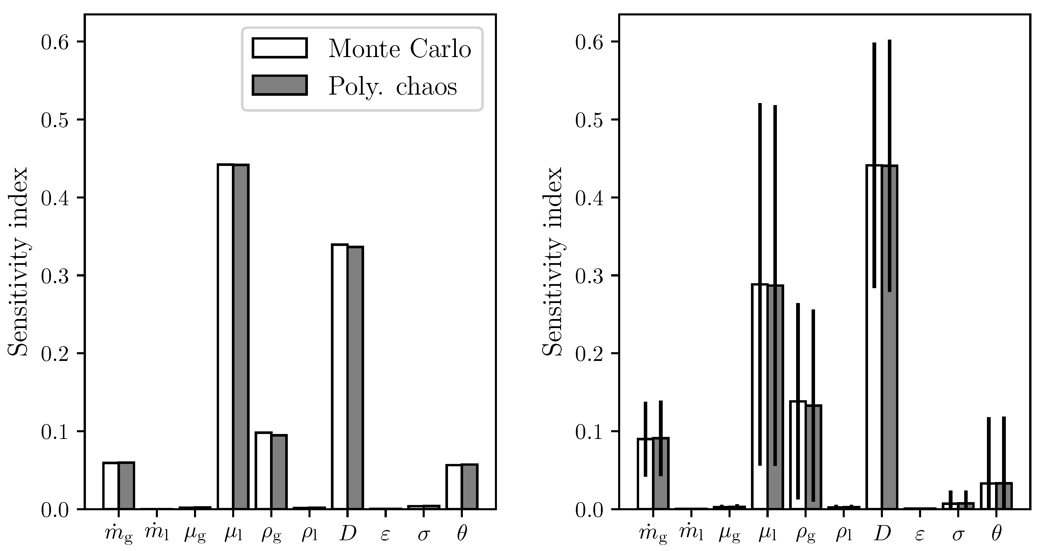
Figure 4 shows the estimated average sensitivity for the holdup predictions. The sensitivities quantify how sensitive the holdup predictions are to each input variable. In other words, it is the contribution of the uncertainty in each input to the uncertainty in holdup predictions. The estimated total sensitivity index and the estimated first-order index never differ more than 0.02. Thus, we use first-order indices in plots and refer to them simply as sensitivities. In the left panel, we see the averages weighted by the variance in each experiment. The right panel gives the plain averages with standard errors. The combined effect of liquid viscosity, pipe diameter and gas density account for ninety percent of the uncertainty in the holdup predictions. We have removed 7 out of the 240 cases from the results because the polynomial chaos expansions for pressure drop do not converge with polynomial order. The criteria for convergence is a change in estimates for the sensitivities, the output mean and the output variance from one order to the next less than 0.01. For the output mean and variance, we use the relative change. The criteria must be reached the latest at order 5.

Table 3. Seven cases where the polynomial chaos expansions for pressure drop do not converge with polynomial order. The first column denotes the variable with the maximal change in the last iteration (absolute change for the sensitivities and relative change for the mean and the variance). The values of that variable for polynomial orders 3–5 are given in the next columns, and the last column gives the regime assigned by the flow model.

Variable	Polynomial Order			Unit	Flow Regime
	3	4	5
$S_D$	0.9961	0.9518	0.9882	−	Bubbly/slug
$S_{T,{\mu }_{\mathrm{l}}}$	0.4814	0.5044	0.5215	−	Slug/stratified
${\mathrm{Var}}_{}\left[\partial p/\partial x\right]$	24.214	24.906	25.196	$P{a}^2/m^2$	Slug/stratified
${\mathrm{Var}}_{}\left[\partial p/\partial x\right]$	28.301	29.042	31.399	$P{a}^2/m^2$	Slug/stratified
${\mathrm{Var}}_{}\left[\partial p/\partial x\right]$	217.10	291.76	269.55	$P{a}^2/m^2$	Slug/stratified
${\mathrm{Var}}_{}\left[\partial p/\partial x\right]$	514.15	528.26	521.32	$P{a}^2/m^2$	Slug/stratified
${\mathrm{Var}}_{}\left[\partial p/\partial x\right]$	5833.6	6555.0	6980.1	$P{a}^2/m^2$	Bubbly/slug

contains information about the pressure drop statistics for the seven cases that do not converge. The holdup statistics actually change less than the threshold of 0.01, but we still exclude these results because we treat the pressure drop and the holdup as a joint variable in the simulations. For each case, we show the variable with the largest change from order 4 to 5 and the values of that variable for order 3, 4 and 5. All seven cases are on the border between two regimes, meaning that the model changes regime based on the sampled measurement error. The regimes assigned by the flow model are listed in the last column of the table.

Figure 5 provides a more refined view of the holdup sensitivities. Each panel gives the histogram of sensitivity to one input based on the 233 cases. We plot separate histograms for slug flow (blue) and stratified flow (red). Furthermore, we compare MC (solid lines) to PC (dotted). There are only small deviations between the two methods. Half of the input variables have sensitivities consistently under 2%. The gas mass rate and density are moderately sensitive, while the diameter and liquid viscosity are in some cases highly sensitive, but not for all cases.

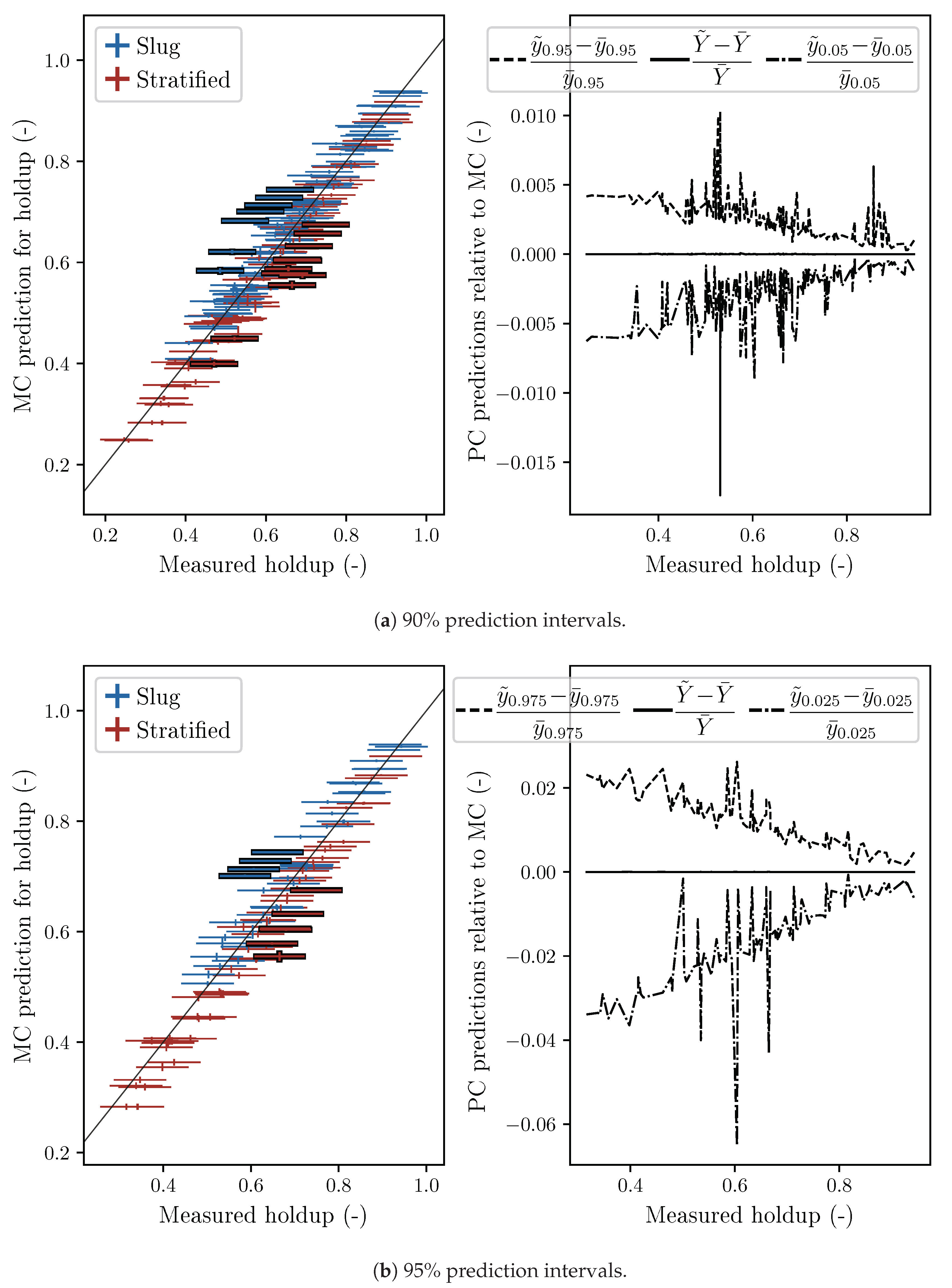
We compare predicted holdup to measured holdup in Figure 6. Only cases with converging prediction intervals from both MC and PC are included. In the left panel, each experiment is drawn as a cross. The horizontal part represents measurement error, and the vertical part (much smaller) represents prediction uncertainty. To be more precise, the crosses are the measured holdup with two standard deviations either way and the predicted mean and interval from MC simulations. The standard deviation in holdup measurements is set to $0.03$. Furthermore, the diagonal line is where measurements and predictions are equal, and cases where the uncertainty box does not cover this line are highlighted. All cases with over-predicted holdup are observed slug flow. Conversely, under-predicted cases are stratified. The 90% intervals do not cover the observations in 20 (10.3%) out of 194 cases, while the 95% intervals are off in 12 (11.4%) out of 105 cases.

The right panels of Figure 6 show the relative difference in the PC predictions and MC predictions. The mean holdup (solid line) is very similar, the upper quantile (dashed) is slightly larger, and the lower quantile (dash-dotted) is slightly smaller with PC. Thus, the PC predictions are overall similar to those of MC, but the intervals are wider.

3.2. Pressure drop

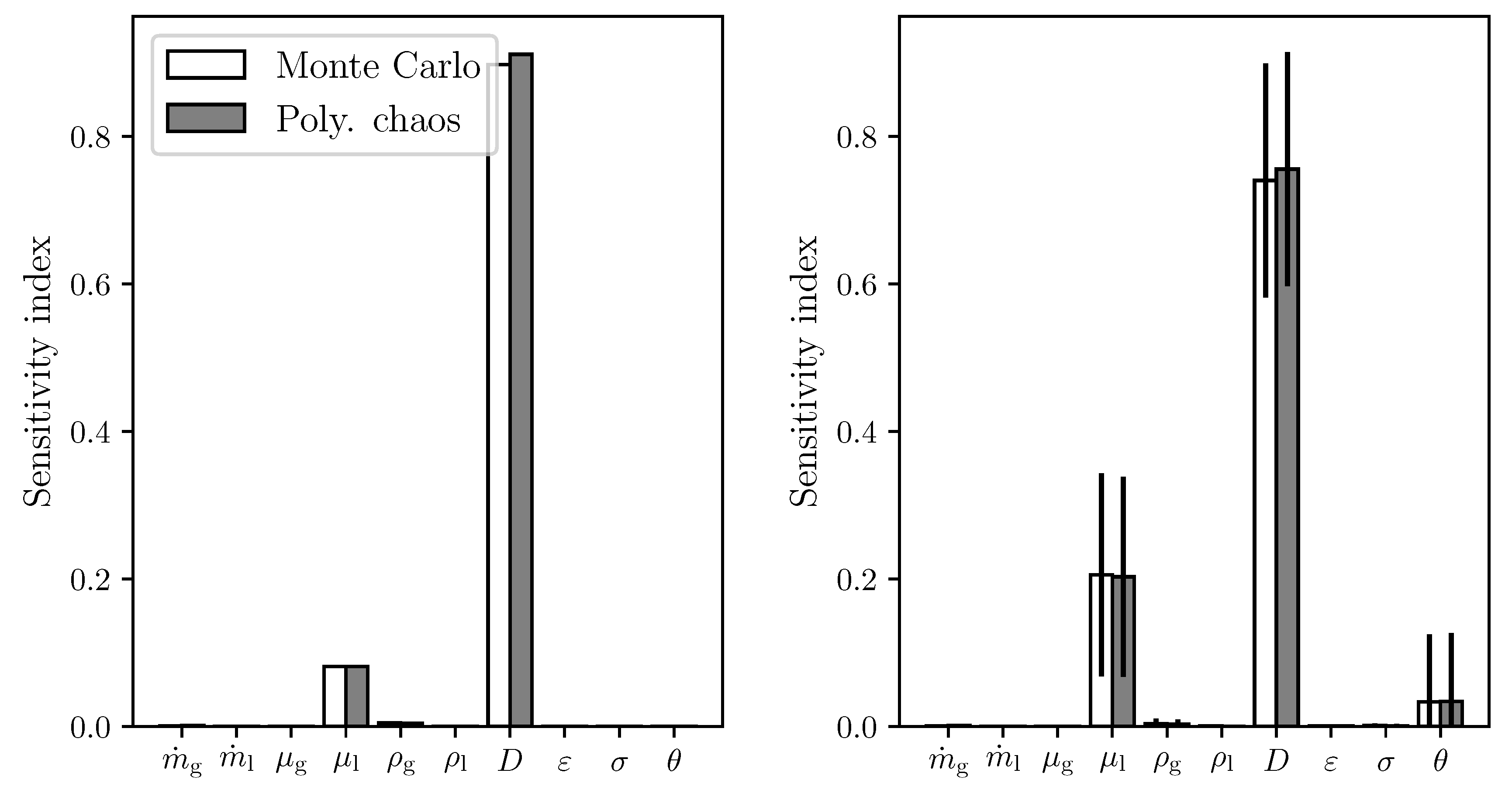
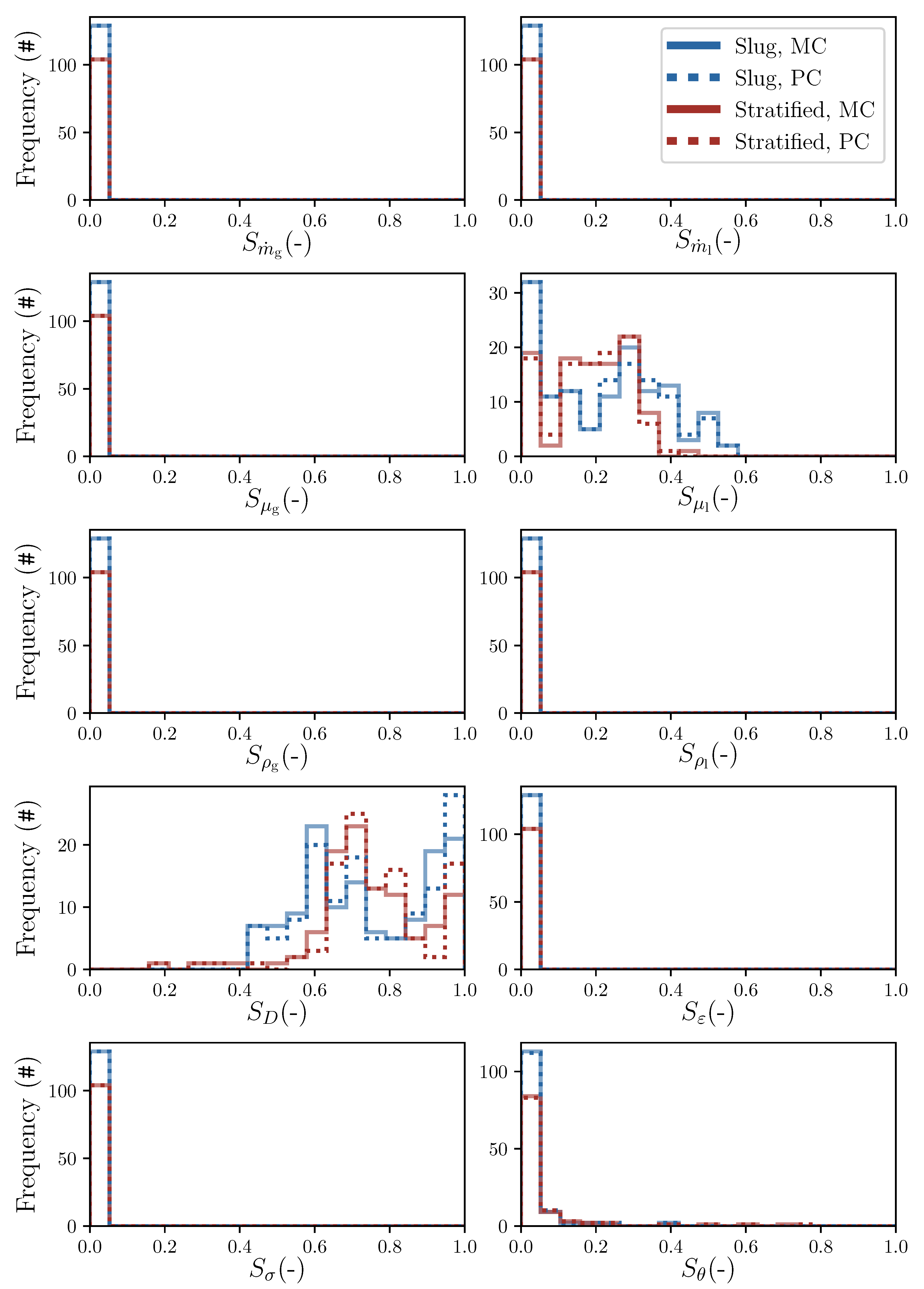
As for holdup, we summarize the pressure drop results in terms of sensitivity and prediction. The averaged sensitivities are given in Figure 7. The weighted average is similar to the plain average. The uncertainty in the diameter measurement is responsible for 90 percent of the uncertainty in pressure drop predictions. The liquid viscosity also contributes, and in some low-variance cases, the pipe inclination. Figure 8 shows the sensitivities by regime. The distributions of sensitivities are similar for stratified flow and slug flow.

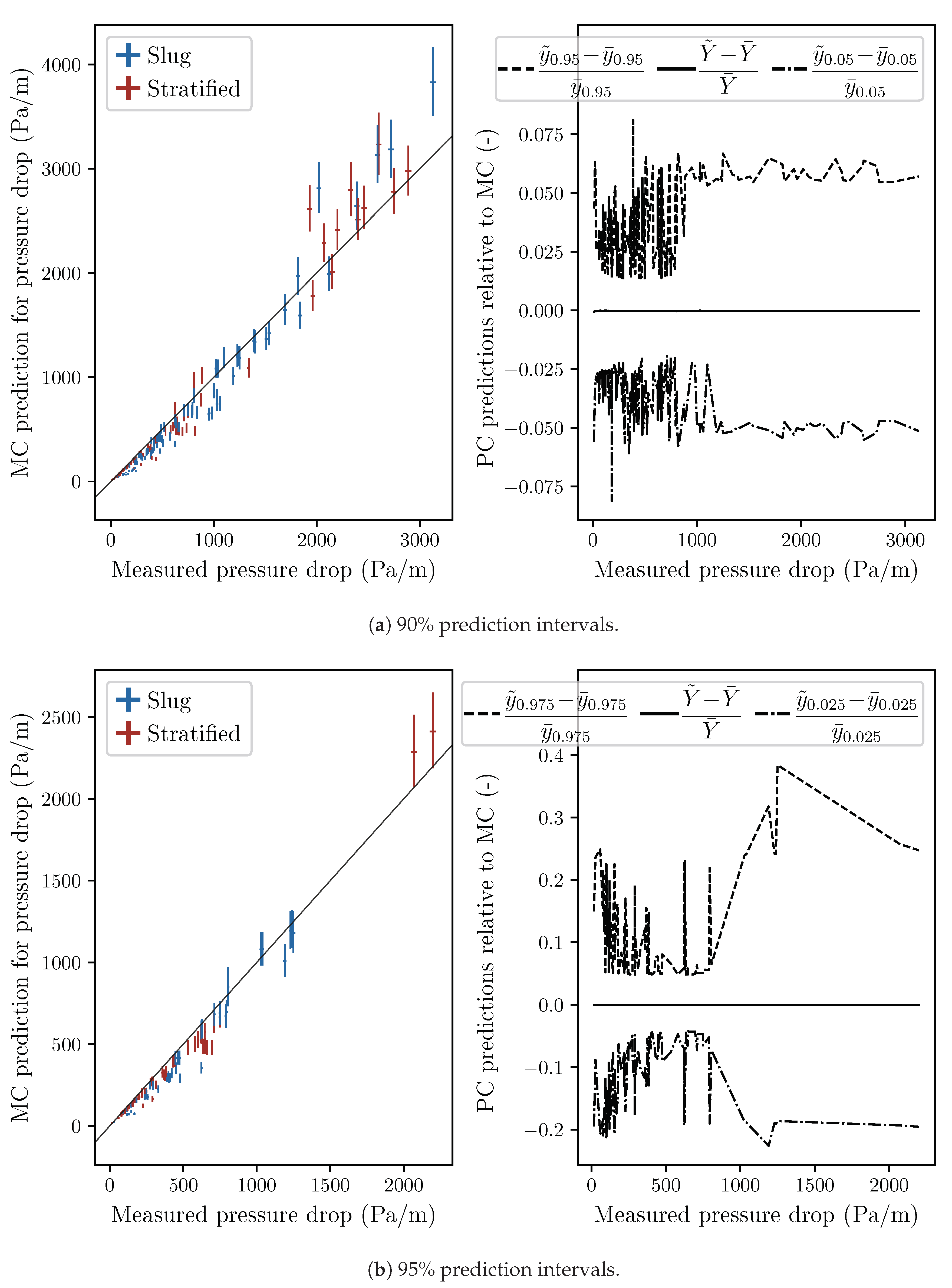
Pressure drop predictions are compared to measurements in Figure 9. Only converged cases are included. The prediction uncertainty is much larger than the measurement uncertainty and increases with the pressure drop. The model under-predicts the pressure drop for small values and over-predicts for large values. The pressure drop predictions are much less accurate than the holdup predictions. The 90% intervals are off in 126 (64.9%) out of 194 cases, while the 95% intervals are off in 62 (59.0%) out of 105 cases.

3.3. Computational Cost

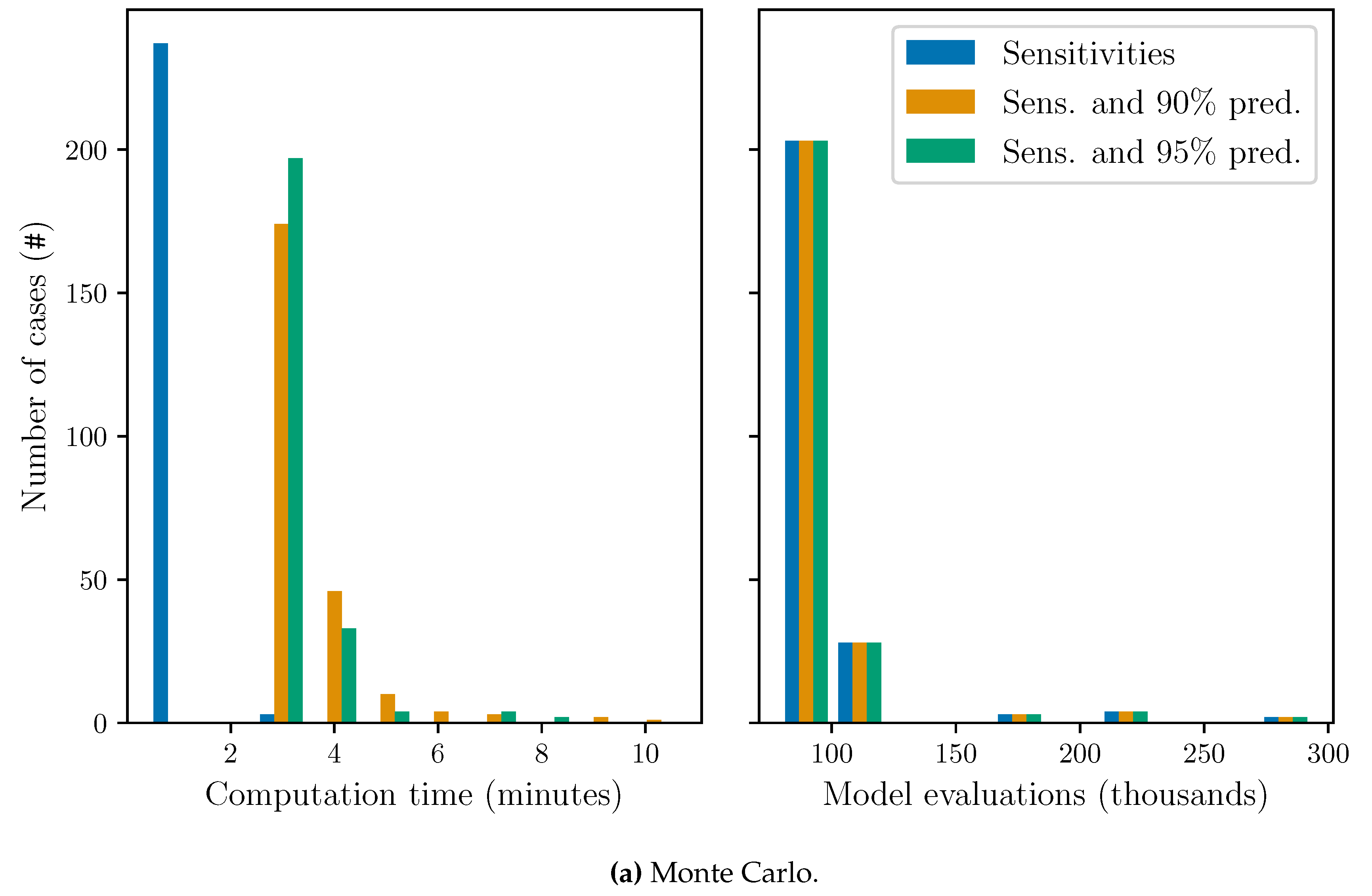
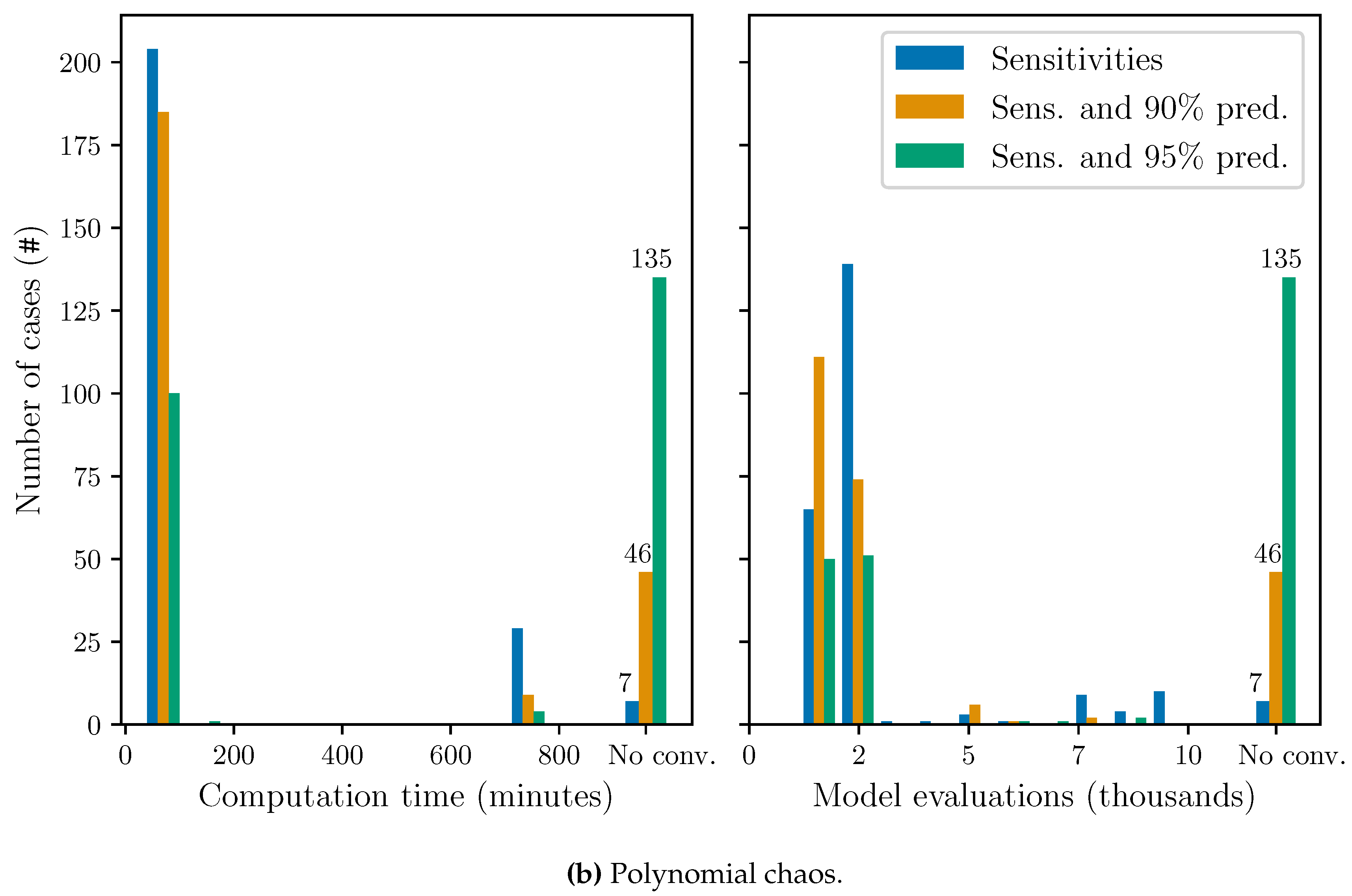
The computational cost of the Monte Carlo simulations is mainly from evaluating the model many times. The polynomial chaos expansion requires fewer model evaluations but also involves large regressions to obtain expansion coefficients. In Figure 10, the computation time (left) and number of model evaluations (right) required for convergence are compared between MC and PC. The colors represent the criteria used for convergence. Blue is only convergence in sensitivities while orange and green is the cost if we also want convergence in prediction intervals on confidence level 90% and 95%, respectively. All cases converge for MC while some do not for PC. The number of cases without convergence is given as an entry on the right hand side. Notice the different scales on the axes for MC and PC.

The computation time is obtained from timing python scripts on the Norwegian HPC infrastructure. We run one MC script and one PC script for each of the 240 cases for each of the three convergence criteria. We terminate each uncertainty analysis at convergence or after 15 h. Thus, the maximum total computation time is $2·240·3·15\mathrm{h}=900$ days. However, because we can run hundreds of scripts in parallel and many cases finish soon, the results are available after one day. We have also implemented the option of parallel evaluations of the model within each script, but chose serial evaluation for this comparison.

4. Discussion

The sensitivity estimates are similar using Monte Carlo or polynomial chaos. The averages $A{S}_i$ gives the clearest picture as they measure how much uncertainty each input brings to the output estimates across all cases. From the first panels of Figure 4 and Figure 7, we see that the pipe diameter and liquid viscosity are important for both pressure drop and holdup, while the gas mass rate, gas density and pipe inclination only matters for the holdup estimates. We can utilize the sensitivity indices for efficiently reducing the uncertainty in the output estimates. The focus should be on reducing the measurement error of the most sensitive variables; in this case, the pipe diameter and the liquid viscosity. Reducing uncertainty in measurements of these variables will efficiently improve predictions. Keep in mind that sensitivity indices are not general but depend on the flow conditions. See Smith et al. [12] for a description of the experiments. The results can not directly be extrapolated to different experiments. A new analysis is required, but the methods described in Section 2 may be applied.

Also note that because first-order and total indices are similar, there are no decisive uncertainty interactions. Furthermore, we cannot conclude that the flow regime is important for sensitivity estimates.

The sensitivities are similar across each regime. However, the moments of the polynomial chaos expansions do not converge with order for some cases on the boundary between regimes. Two cases are on the boundary bubbly/slug and neither converge with PC. Among 24 cases on the boundary slug/stratified, five cases do not converge with PC. Thus, the current implementation of PC expansions is unreliable on the regime boundaries. The expansions do not capture the behavior of the flow model well on the boundaries because the model is not smooth there. Adding higher-order terms to the expansion would make the expansion better resemble non-smooth behavior, but this is not immediately possible due to computational expense. It is possible to construct high-order approximations with low complexity by applying variable selection, but this approach is less applicable.

We have also explored the technical details in the uncertainty computations, specifically the performance of Monte Carlo simulations compared to that of polynomial chaos methods. For the fluid model in question, we clearly prefer MC because this method provides uncertainty estimates for all cases, and it does so in the least amount of time. In contrast, PC fails in many cases and has a larger computation cost. The strength of PC lies in the low number of required model evaluations. Compared to MC, polynomial chaos is likely to perform better if the fluid model required more time for each evaluation.

We have compared measured holdup with predicted holdup accounting for uncertainty in both. The equivalent comparison was applied to the pressure drop. The holdup prediction matches the measured values well. We can observe that over-predicted cases are slug flow and under-predicted cases are stratified. The predictions of pressure drops are less accurate, with under-prediction for small values and over-prediction for large pressure drops. There is a clear bias in the estimates, which suggests there are physics that are not captured by the model. The authors of Smith et al. [36] pointed to the over-prediction of the slug velocity variable $C_0$. The claim is supported by follow-up experiments, which they discuss in their Section 3.3.

In summary, estimates for sensitivities and output predictions using MC are similar to those of PC, and the pipe diameter and the liquid viscosity have the largest sensitivity indices. The Monte Carlo method is preferred because it is more robust and requires less time. This conclusion applies to the flow model used and the implementation of each uncertainty method. The uncertainty analysis also provides evidence that holdup predictions are accurate, while pressure drop predictions are biased.

Future Research

We have seen that half of the input variables contribute less than 2% to the output uncertainty in all cases. For polynomial chaos, it is possible to construct the polynomial approximation by attempting to prioritize the important variables. One idea is to iteratively introduce higher order polynomials in significant variables. This way, we can reach a sufficiently high polynomial order without introducing too many regressors.

Applying the methods of Hoyer et al. [5] to create probability distributions for closure laws will make the analysis of the uncertainty in the flow model more complete. Currently, the closure laws are treated as known. We think it is possible to tune the closure law distributions by comparing the output predictions with measurements. An applicable tuning method is the minimum continuous ranked probability score (CRPS) estimation, as demonstrated in Gneiting et al. [37].

References

1. Lee, S.H.; Chen, W. A comparative study of uncertainty propagation methods for black-box-type problems. Struct. Multidiscipl. Optim. 2009, 37, 239. [Google Scholar] [CrossRef]
2. Cremaschi, S.; Kouba, G.E.; Subramani, H.J. Characterization of confidence in multiphase flow predictions. Energ. Fuel. 2012, 26, 4034–4045. [Google Scholar] [CrossRef]
3. Holm, H.; Saha, P.; Suleymanov, V.; Vanvik, T.; Hoyer, N. Shtokman flow assurance challenges—A systematic approach to analyze uncertainties–Part 1. In Proceedings of the 15th International Conference on Multiphase Production Technology, Cannes, France, 15–17 June 2011. [Google Scholar]
4. Holm, H.; Saha, P.; Suleymanov, V.; Vanvik, T.; Hoyer, N. Shtokman flow assurance challenges—A systematic approach to analyze uncertainties–Part 2. In Proceedings of the 15th International Conference on Multiphase Production Technology, Cannes, France, 15–17 June 2011. [Google Scholar]
5. Hoyer, N.; Kirkedelen, M.; Biberg, D.; Johnson, G.; Valle, A.; Johansson, P.; Nossen, J. A structured approach for the evaluation of uncertainties in flow assurance systems. In Proceedings of the 16th International Conference on Multiphase Production Technology, Cannes, France, 12–14 June 2013. [Google Scholar]
6. Klavetter, K.; Posluszny, D.; Warr, J.; Cremaschi, S.; Sarica, C.; Subramani, H. Uncertainty analysis of multiphase flow models: A comparison of three propagation approaches. In Proceedings of the 8th North American Conference on Multiphase Technology, Banff, AB, Canada, 20–22 June 2012. [Google Scholar]
7. Keinath, B. Decision analysis in multiphase flow: Uncertainty, risk and application. In Proceedings of the 18th International Conference on Multiphase Production Technology, Cannes, France, 7–9 June 2017. [Google Scholar]
8. Liu, Y.; Dinh, N.T.; Smith, R.C.; Sun, X. Uncertainty quantification of two-phase flow and boiling heat transfer simulations through a data-driven modular Bayesian approach. Int. J. Heat. Mass. Tran. 2019, 138, 1096–1116. [Google Scholar] [CrossRef]
9. Picchi, D.; Poesio, P. Uncertainty quantification and global sensitivity analysis of mechanistic one-dimensional models and flow pattern transition boundaries predictions for two-phase pipe flows. Int. J. Multiphas. Flow 2017, 90, 64–78. [Google Scholar] [CrossRef]
10. Klinkert, J. The characterization of Uncertainty for Steady State Multiphase Flow Models in Pipelines. Master’s Thesis, Delft University of Technology, Delft, The Netherlands, 19 January 2018. [Google Scholar]
11. Lataniotis, C.; Marelli, S.; Sudret, B. Uqlab User Manual—The Input Module. 2015. Available online: https://www.researchgate.net/profile/Bruno_Sudret/publication/281232688_UQLab_user_manual_-_the_INPUT_module/links/55dc1df708ae9d6594937608.pdf (accessed on 26 February 2020).
12. Smith, I.E.; Nossen, J.; Unander, T.E. Improved holdup and pressure drop predictions for multiphase flow with gas and high viscosity oil. In Proceedings of the 16th International Conference on Multiphase Production Technology, Cannes, France, 12–14 June 2013. [Google Scholar]
13. Lichota, P.; Szulczyk, J.; Tischler, M.B.; Berger, T. Frequency Responses Identification from Multi-Axis Maneuver with Simultaneous Multisine Inputs. J. Guid. Contr. Dynam. 2019, 42, 2550–2556. [Google Scholar] [CrossRef]
14. Lichota, P.; Noreña, D.A. A priori model inclusion in the multisine maneuver design. In Proceedings of the 17th International Carpathian Control Conference (ICCC), Tatranska Lomnica, Slovakia, 29 May–1 June 2016; pp. 440–445. [Google Scholar]
15. Chen, S.; Wang, X.; Harris, C.J. NARX-based nonlinear system identification using orthogonal least squares basis hunting. IEEE Trans. Contr. Syst. Tech. 2007, 16, 78–84. [Google Scholar] [CrossRef] [Green Version]
16. Efremov, A. System Identification Based on Stepwise Regression for Dynamic Market Representation. In Proceedings of the International Conference on Data Mining and Knowledge Engineering, Rome, Italy, 29 April 2010; Volume 4, pp. 28–30. [Google Scholar]
17. Dukler, A.E.; Hubbard, M.G. A model for gas-liquid slug flow in horizontal and near horizontal tubes. Ind. Eng. Chem. Fund. 1975, 14, 337–347. [Google Scholar] [CrossRef]
18. Gregory, G.; Nicholson, M.; Aziz, K. Correlation of the liquid volume fraction in the slug for horizontal gas-liquid slug flow. Int. J. Multiphas. Flow 1978, 4, 33–39. [Google Scholar] [CrossRef]
19. Kora, C.; Sarica, C.; Zhang, H.q.; Al-Sarkhi, A.; Al-Safran, E. Effects of high oil viscosity on slug liquid holdup in horizontal pipes. In Proceedings of the Canadian Unconventional Resources Conference, Calgary, AB, Canada, 15–17 November 2011. [Google Scholar]
20. Bendiksen, K.H. An experimental investigation of the motion of long bubbles in inclined tubes. Int. J. Multiphas. Flow 1984, 10, 467–483. [Google Scholar] [CrossRef] [Green Version]
21. Jeyachandra, B.; Gokcal, B.; Al-Sarkhi, A.; Sarica, C.; Sharma, A. Drift-velocity closure relationships for slug two-phase high-viscosity oil flow in pipes. SPE J. 2012, 17, 593–601. [Google Scholar] [CrossRef]
22. Nuland, S. Bubble front velocity in horizontal slug flow with viscous Newtonian, shear thinning and Bingham fluids. In Proceedings of the 3rd International Conference on Multiphase Flow (ICMF’98), Lyon, France, 8–12 June 1998. [Google Scholar]
23. Hinze, J.O. Turbulence; McGraw-Hill: New York, NY, USA, 1975; Volume 2. [Google Scholar]
24. Andreussi, P.; Persen, L. Stratified gas-liquid flow in downwardly inclined pipes. Int. J. Multiphas. Flow 1987, 13, 565–575. [Google Scholar] [CrossRef]
25. White, F.M. Fluid Mechanics; McGraw-Hill: New York, NY, USA, 2011. [Google Scholar]
26. Brkić, D.; Praks, P. Accurate and efficient explicit approximations of the Colebrook flow friction equation based on the Wright ω-function. Mathematics 2019, 7, 34. [Google Scholar] [CrossRef] [Green Version]
27. Khaledi, H.A.; Smith, I.E.; Unander, T.E.; Nossen, J. Investigation of two-phase flow pattern, liquid holdup and pressure drop in viscous oil–gas flow. Int. J. Multiphas. Flow 2014, 67, 37–51. [Google Scholar] [CrossRef]
28. ISO, I.; OIML, B. Guide to the Expression of Uncertainty in Measurement. 1995. Available online: https://www.bipm.org/utils/common/documents/jcgm/JCGM_100_2008_E.pdf (accessed on 26 February 2020).
29. Sobol, I.M. Sensitivity estimates for nonlinear mathematical models. Math. Model. Comput. Exp. 1993, 1, 407–414. [Google Scholar]
30. Saltelli, A.; Annoni, P.; Azzini, I.; Campolongo, F.; Ratto, M.; Tarantola, S. Variance based sensitivity analysis of model output. Design and estimator for the total sensitivity index. Comput. Phys. Comm. 2010, 181, 259–270. [Google Scholar] [CrossRef]
31. Saltelli, A. Making best use of model evaluations to compute sensitivity indices. Comput. Phys. Comm. 2002, 145, 280–297. [Google Scholar] [CrossRef]
32. Sobol, I.M.; Tarantola, S.; Gatelli, D.; Kucherenko, S.; Mauntz, W. Estimating the approximation error when fixing unessential factors in global sensitivity analysis. Reliab. Eng. Syst. Saf. 2007, 92, 957–960. [Google Scholar] [CrossRef]
33. Jansen, M.J. Analysis of variance designs for model output. Comput. Phys. Comm. 1999, 117, 35–43. [Google Scholar] [CrossRef]
34. Xiu, D. Numerical Methods for Stochastic Computations: A Spectral Method Approach; Princeton university press: Princeton, NJ, USA, 2010. [Google Scholar]
35. Feinberg, J.; Langtangen, H.P. Chaospy: An open source tool for designing methods of uncertainty quantification. J. Comput. Sci. 2015, 11, 46–57. [Google Scholar] [CrossRef] [Green Version]
36. Smith, I.E.; Nossen, J.; Kjølaas, J.; Lund, B. Development of a Steady-State Point Model for Prediction of Gas/Oil and Water/Oil Pipe Flow. J. Dispers. Sci. Technol. 2015, 36, 1394–1406. [Google Scholar] [CrossRef]
37. Gneiting, T.; Raftery, A.E.; Westveld III, A.H.; Goldman, T. Calibrated probabilistic forecasting using ensemble model output statistics and minimum CRPS estimation. Mon. Weather Rev. 2005, 133, 1098–1118. [Google Scholar] [CrossRef]
Sample Availability: Code and data are available online: https://dataverse.no/dataset.xhtml?persistentId=doi:10.18710/OWKABR.
Figure 1. Slug flow. Gas bubbles are separated by liquid slugs. At the near end of the pipe, we have illustrated the gas–wall perimeter S g (black dashed line), liquid–wall perimeter S l (black line) and the interface perimeter S i (white line).
Algorithms 13 00053 g001
Figure 2. Flowchart of the point model. First holdup is computed, then pressure drop.
Algorithms 13 00053 g002
Figure 3. Comparison of two methods of interpolation by Reynolds number. (Left) Histograms of holdup for small perturbation of input around Re ≈ 3000 for the original model (blue) and the modified model (orange). (Right) The bubble nose variable C0(Re) in the transition from laminar to turbulent for the original model (blue line) and the modified model (orange dashed line).
Algorithms 13 00053 g003
Figure 4. Holdup sensitivity estimates averaged over 233 experiments. (Left) Weighted by the variance in each experiment. (Right) Plain averages with standard error bars.
Algorithms 13 00053 g004
Figure 5. Frequency histograms of the holdup sensitivity estimates across 233 experiments. The sensitivity distribution for one input variable is given in each panel. The experiments are categorized as slug (blue) or stratified (red) and we compare estimates from Monte Carlo (solid lines) and PC (dotted).
Algorithms 13 00053 g005
Figure 6. (Left) Predicted versus measured holdup for 194 experiments. The diagonal line is where the coordinates are equal, and cases with a discrepancy between prediction and observation are highlighted. The first axis gives measured value with two standard errors either way. The second axis is predicted mean, lower quantile and upper quantile. Slug experiments are blue and stratified ones are red. (Right) The relative difference in PC predictions compared to MC predictions with respect to measured holdup. Upper quantiles (dashed), means (solid) and lower quantiles (dash-dotted).
Algorithms 13 00053 g006
Figure 7. Pressure drop sensitivity estimates averaged over 233 experiments. (Left) Weighted by the variance in each experiment. (Right) Plain averages with standard error bars.
Algorithms 13 00053 g007
Figure 8. Frequency histograms of the pressure drop sensitivity estimates across 233 experiments. The sensitivity distribution for one input variable is given in each panel. The experiments are categorized as slug (blue) or stratified (red), and we compare estimates from Monte Carlo (solid lines) and PC (dotted).
Algorithms 13 00053 g008
Figure 9. (Left) Predicted versus measured pressure drop for 194 experiments. The diagonal line is where the coordinates are equal. The first axis gives measured value with two standard errors either way. The second axis is predicted mean, lower quantile and upper quantile. Slug experiments are blue, and stratified ones are red. (Right) The relative difference in PC predictions compared to MC predictions with respect to measured pressure drop. Upper quantiles (dashed), means (solid) and lower quantiles (dash-dotted).
Algorithms 13 00053 g009
Figure 10. Frequency histogram of computational cost across 240 experiments. Each color is one type of simulation criterion, namely only convergence in sensitivities (blue) or also 90% prediction intervals (orange) or 95% (green). The number of cases that did not converge is given as an entry on the right. (Left) Computation time. (Right) Number of model evaluations.
Algorithms 13 00053 g010aAlgorithms 13 00053 g010b