Feasibility Pump Algorithm for Sparse Representation under Gaussian Noise

Abstract

In this paper, the Feasibility Pump is adapted for the problem of sparse representations of signals affected by Gaussian noise. This adaptation is tested and then compared to Orthogonal Matching Pursuit (OMP) and the Fast Iterative Shrinkage-Thresholding Algorithm (FISTA). The feasibility pump recovers the true support much better than the other two algorithms and, as the SNR decreases and the support size increases, it has a smaller recovery and representation error when compared with its competitors. It is observed that, in order for the algorithm to be efficient, a regularization parameter and a weight term for the error are needed.

1. Problem Formulation

The sparse representation of a signal $y\in {\mathbb{R}}^m$ is the solution $x\in {\mathbb{R}}^n$ with the smallest number of nonzero elements to the under-determined system $y=Dx$, where $D\in {\mathbb{R}}^{m\times n}$, $m<n$, is a given matrix named dictionary. Since in most cases noise is involved, the data misfit measure is minimized. Also, rather than attempting to find the sparsest solution, it is easier to bound the number of nonzero elements by a given threshold K and so the sparse representation can be found by solving the optimization problem

$$\begin{array}{cccc}\hfill & \underset{x\in {\mathbb{R}}^n}{\mathrm{minimize}}\hfill & \hfill & {\parallel y-Dx\parallel }_2\hfill \\ \hfill & \mathrm{subject}\mathrm{to}\hfill & \hfill & {\parallel x\parallel }_0\le K.\hfill \end{array}$$

(1)

Since the 2-norm is involved, the assumption is that the noise is Gaussian. This is still an NP-hard problem.

A common way to treat (1) is to replace the $l_0$ norm with the $l_1$ norm, thus relaxing the problem to a convex one. Transferring also the constraint into the objective, the result is a lasso style problem:

$$\begin{array}{cccc}\hfill & \underset{x\in {\mathbb{R}}^n}{\mathrm{minimize}}\hfill & \hfill & {\parallel y-Dx\parallel }_2^2+\lambda {\parallel x\parallel }_1.\hfill \end{array}$$

(2)

A less used approach takes into account the fact that the number of non-zero coefficients in (1) is bounded using the $l_0$ norm, hence Mixed Integer Programming (MIP) algorithms can be considered to solve the problem as it is posed, using either an integer variable for the number of coefficients or the binary decision whether a coefficient is used for the representation or not.

The Feasibility Pump (FP), proposed in References [1,2], is an MIP algorithm that alternates between solving the problem with relaxed integer constraints and the one satisfying the integer requirements. This is done until a point is reached that satisfies all the constraints, even though it might be not optimal, or for a prescribed number of iterations. The Feasibility Pump begins at an initial solution and then proceeds through several iterations to minimize the difference between the solutions of the alternating problems. Several modifications and improvements [3,4,5,6,7,8,9,10] have been proposed for this algorithm. See the bibliography in Reference [11] for a more extensive image. The case in which the $l_1$ norm is used for the representation error was analyzed and a modification of the Feasibility Pump algorithm for this problem was presented in Reference [12].

We propose to combine the MIP approach with the lasso problem (2). The binary variable $b\in {\{0,1\}}^n$ is introduced to perform the role of an indicator that shows which atom of the dictionary D is used for the representation of y. We then combine (1) with (2) to obtain the problem

$$\begin{array}{cc}\underset{x\in {\mathbb{R}}^n,b\in {\{0,1\}}^n}{\mathrm{minimize}}\hfill & {\parallel y-Dx\parallel }_2^2+\lambda {\parallel x\parallel }_1\hfill \\ \mathrm{subject}\mathrm{to}\hfill & 1_n^{T}b\le K\hfill \\ \hfill & -Mb\le x\le Mb,\hfill \end{array}$$

(3)

where $1_n$ is a vector of length n whose elements are all equal to 1. The $l_1$ regularization enforces the sparsity condition on the representation x, as the $l_1$ norm favors sparsity, and helps the convergence of the Feasibility Pump algorithm, which will be used as an (approximate) MIP solver. As in Reference [13], a pioneer of MIP techniques for sparse representations, the big-M trick is employed in (3), where M is a preset parameter chosen as $M=1.1\parallel D^T{y\parallel }_{\infty }/{\parallel D\parallel }_2^2$. This is used to bound the size of the representation coefficients. Note that if $b=0$, then $x=0$; if $b=1$, then x is practically free, since the constraint $\left|x\right|\le M$ is of no consequence due to the large value of M.

Finally, to implement problem (3), an auxiliary variable $w\in {\mathbb{R}}^n$ is introduced for the regularization term, resulting in

$$\begin{array}{cc}\underset{x\in {\mathbb{R}}^n,w\in {\mathbb{R}}^n,b\in {\{0,1\}}^n}{\mathrm{minimize}}\hfill & x^T{D}^{T}Dx-2y^{T}Dx+\lambda 1_n^{T}w\hfill \\ \mathrm{subject}\mathrm{to}\hfill & 1_n^{T}b\le K\hfill \\ \hfill & -w\le x\le w\hfill \\ \hfill & w\le Mb.\hfill \end{array}$$

(4)

In this paper, the focus is on the implementation of the Feasibility Pump of problem (4). Our solution is based on the Objective FP, originated in Reference [3]. Section 2 presents our Feasibility Pump algorithm and the implementation details. Section 3 is dedicated to experimental results showing the behavior of our algorithm and comparisons with the Orthogonal Matching Pursuit (OMP) and Fast Iterative Shrinkage-Thresholding (FISTA) algorithms. We show that our regularized Feasibility Pump algorithm is consistently better when compared to the other algorithms. Section 4 presents the conclusions and future ideas for research.

2. Algorithm

Algorithm 1 solves the reformulation (4) of problem (1). It is similar in structure to that in Reference [12], although the underlying optimization problem and some important details are different. We will point out the differences when they are presented.

The Feasibility Pump algorithm starts with the computation of the solution for the relaxed version of the initial problem (4), where b takes values in the ${[0,1]}^n$ interval, instead of being a binary variable. The problem becomes convex; more precisely, it belongs to quadratic programming; the MATLAB function quadprog is used to solve it, based on an interior-point algorithm; other solvers or packages could be used as well.

The real solution b is rounded to the vector $\tilde{b}\in {\{0,1\}}^n$. The largest K elements of b are rounded upwards to 1, while the others are rounded downwards to 0. Indirectly, a sparse solution is obtained with exactly K elements.    

Algorithm 1: Modified Feasibility Pump.

In each iteration of the Feasibility Pump, the vector b and the tentative solution x are updated by solving

$$\begin{array}{cc}\underset{x\in {\mathbb{R}}^n,w\in {\mathbb{R}}^n,b\in {[0,1]}^n}{\mathrm{minimize}}\hfill & (1-\alpha )\Delta (b,\tilde{b})+\alpha \left[\frac{K}{er{r}_{init}^2}(x^T{D}^{T}Dx-2y^{T}Dx)+\lambda 1_n^{T}w\right]\hfill \\ \mathrm{subject}\mathrm{to}\hfill & 1_n^{T}b\le K\hfill \\ \hfill & -w\le x\le w\hfill \\ \hfill & w\le Mb,\hfill \end{array}$$

(5)

where $\Delta (b,\tilde{b})={\parallel b-\tilde{b}\parallel }_1$ and $er{r}_{init}$ is the representation error at the initial Feasibility Pump step (4). This quadratic programming problem is also solved with quadprog in MATLAB. The iteration step has an objective that combines the representation error ${\parallel y-Dx\parallel }_2$ with a term that enforces the new solution b to be near from the current integer vector $\tilde{b}$, with the aim of making the solution b nearer from a binary vector. This kind of modification, named Objective FP, is proposed in Reference [3] and is essential in our case for finding good values of the objective; feasibility is easy to obtain, since rounding always gives a K-sparse solution, and so the original FP [1] would always converge in one iteration, possibly to a poor solution.

After each iteration, the parameter $\alpha$ is reduced and the integer condition will weigh more than the error objective. The reduction of $\alpha$ is done by multiplication with a value $\gamma \in (0,1)$:

$$\alpha \leftarrow \gamma \alpha .$$

(6)

A large $\gamma$ will give the smallest error, but the execution time is longer, while a smaller $\gamma$ offers faster results, but with a larger error.

During our tests, it was observed that the addition of the factor $\frac{K}{er{r}_{init}^2}$ in (5) is necessary to increase the influence of the error in the optimization process because the error is much smaller than the $\Delta (b,\tilde{b})$ and ${\parallel x\parallel }_1$ terms and it needs an additional weight parameter. The division with the square of the error removes the difference of the orders in magnitude between the $\Delta (b,\tilde{b})$ term, regularization term and the error term during the first iteration steps. With each iteration the importance of the error terms decays. Without the weight, the importance of the error term decays too fast and has little effect in the optimization process; the weight is used so that the error term plays an important role for more iterations of the algorithm. The factor K is added such that the error term is as important as the $\Delta (b,\tilde{b})$ term for more time, as $\alpha$ decreases the importance of the error term. It also helps the choice of $\lambda$. As $0\le \Delta (b,\tilde{b})\le 2K$, with $2K$ being nearly impossible to attain, the multiplication with K puts both the error and the feasibility term on similar weights; without the K value, the square error would only normalize the error term, while the magnitude of the $\Delta (b,\tilde{b})$ term would act as a weight that forces the algorithm to focus more on getting a sparse solution, than on reducing the representation error. We note that directly using the algorithm from Reference [12], without the factor $\frac{K}{er{r}_{init}^2}$, leads to poor results. Balancing the terms of the objective, like we did in (5), is also done in Reference [9], but with different means.

The regularization term ${\parallel x\parallel }_1$ has a double role. It helps enforce the desired sparsity and also helps the algorithm to converge when the dictionary is ill conditioned. The lack of the regularization term increases the running time of the algorithm, sometimes not even reaching convergence. The $\lambda$ tuning parameter is very important as it influences heavily the performance of the model, as shown in Reference [14]. Note that at the end of Algorithm 1, when the support is settled, the regularization term is removed and the (optimal) least squares solution corresponding to that sparse support is computed; such a feature was not present in Reference [12].

The perturbation strategy used when cycles occur in the Feasibility Pump iterative process is similar to the one used in Reference [12]; it belongs to the category of strong perturbations, as all elements of $\tilde{b}$ are perturbed. Inspired by Reference [6], we consider that a cycle appears when one of the following conditions is met (we use index t for the current iteration and $t-1$ for the previous one): (i) $\tilde{b}$ is the same as in the previous iteration and $|{\alpha }_t-{\alpha }_{t-1}|<{10}^{-3}$ (note that even if $\tilde{b}$ is the same, different values of $\alpha$ lead to different solutions in (5)), (ii) $\parallel b_t-b_{t-1}\parallel <{10}^{-4}$, (iii) $\parallel b_t-b_{t-1}\parallel \ge 0.9\parallel b_{t-1}-b_{t-2}\parallel$; the last two conditions take into account both the absolute value of $\parallel b_t-b_{t-1}\parallel$ and its relative change with respect to the previous iteration.

The algorithm described above is named Sparse Quadratic Feasibility Pump (SQFP). Unlike the Branch and Bound algorithms from Reference [13], SQFP may not attain the optimal solution, but it has a running time that is comparable with those of popular algorithms for sparse representation. In contrast, the MIP algorithms from Reference [13] may be extremely slow for some problems.

3. Results

In order to obtain numerical results, the testing scheme from Reference [12] is used, with the significant distinction that noise is now Gaussian.

In a first test, for which we report extensive results, we use randomly generated dictionaries with condition numbers of 100, 1000, 10,000 and 100,000. For each condition number, 160 dictionaries of size $80\times 200$ are generated. The test signals are obtained with $y=D{x}_{\mathrm{true}}+u$, where the solutions $x_{\mathrm{true}}$ have $K\in \{5,7,9,11\}$ nonzero coefficients generated randomly following a Gaussian distribution, in random positions; the noise u is Gaussian and its variance is chosen such that the signal to noise ratios have values $10,20,30$, ∞.

For the computation of the representation error, the relative error

$$\begin{array}{ccc}\hfill & \hfill & \hfill e=\frac{{\parallel Dx-y\parallel }_2}{{\parallel y\parallel }_2}\end{array}$$

(7)

is used (where now x is the computed solution), in accordance with the formulation of the initial problem (1).

We have implemented SQFP as shown in Algorithm 1. The initial weight $\alpha$ is set to 1 and is multiplied by an update factor $\gamma =0.9$ at each iteration; these values seem to provide a good compromise between convergence speed and representation error. The number of iterations $Iter$ is set to 1000. We run SQFP with 50 equally spaced values of the regularization parameter $\lambda$ from 0 to 1. The value for which the mean representation error is the smallest is considered the best choice for $\lambda$.

Several types of algorithms have been proposed [15] to find the solution of (1) or its relaxed version (2). The OMP (Orthogonal Matchmaking Pursuit) [16] and the FISTA (Fast Iterative Shrinkage-Thresholding Algorithm) [17] algorithms where chosen for comparison as they are some of the most commonly used.

Both FISTA and SQFP use the regularization parameter $\lambda$. FISTA is tested with 500 equally spaced values between 0 to 0.05.

The algorithms are implemented in MATLAB and tested on a computer with a 6-core 3.4 GHz processor and 32 GB of RAM.

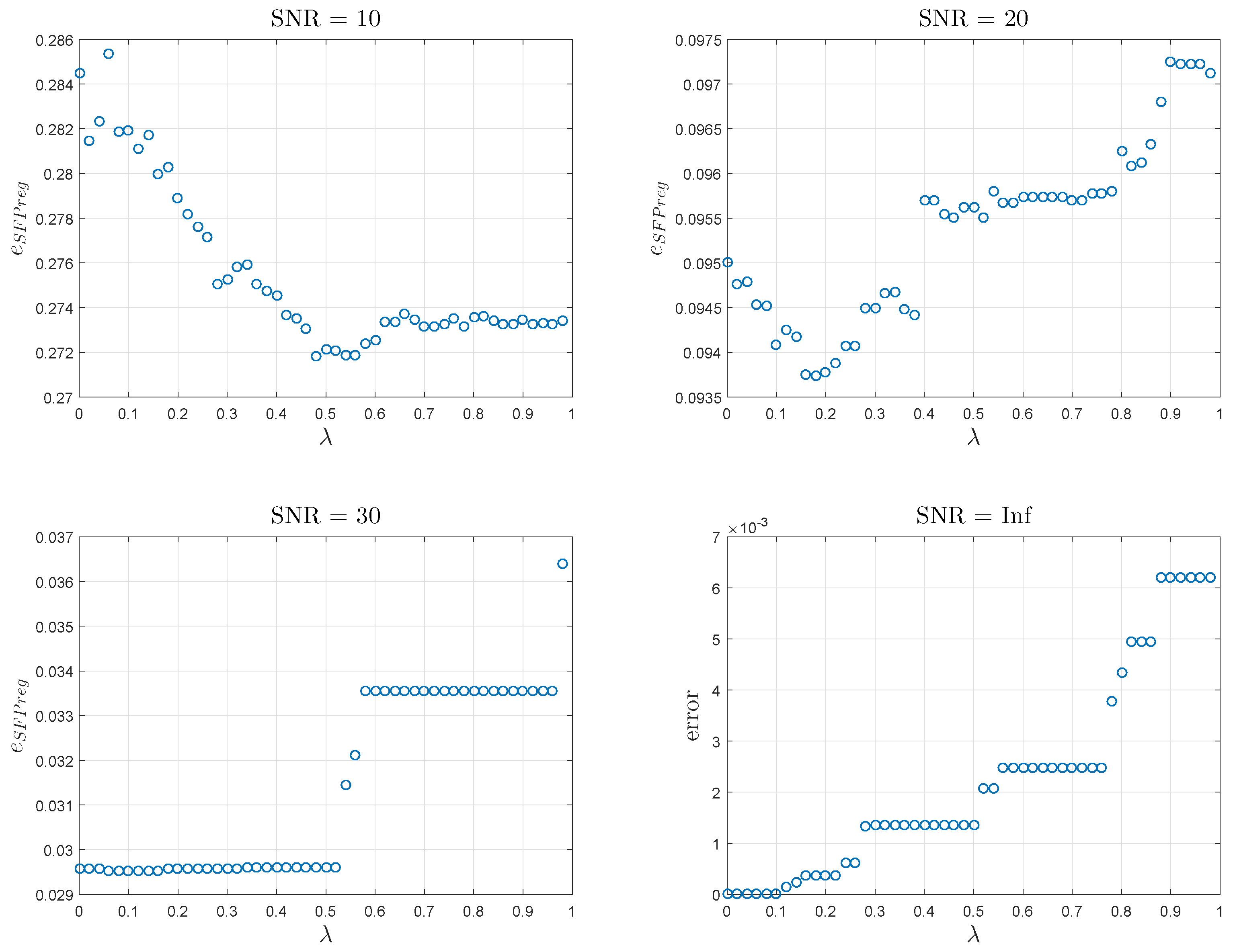
The variation of the error produced by SQFP depending on $\lambda$ is represented in Figure 1 for $K=11$ and condition number 1000. It can be seen that for the lower SNR values, the error has a relatively well defined minimum around $\lambda =0.5$ for $SNR=10$ and $\lambda =0.18$ for $SNR=20$. From the minimum point the error increases as $\lambda$ increases. For the larger SNR values, the error is very small in the beginning, with small variations as $\lambda$ increases from zero; after a certain value the error increases a lot. In these cases regularization offers very small benefits.

Figure 1. Mean representation error depending on $\lambda$ for $K=11$, for matrix conditioning of 1000.

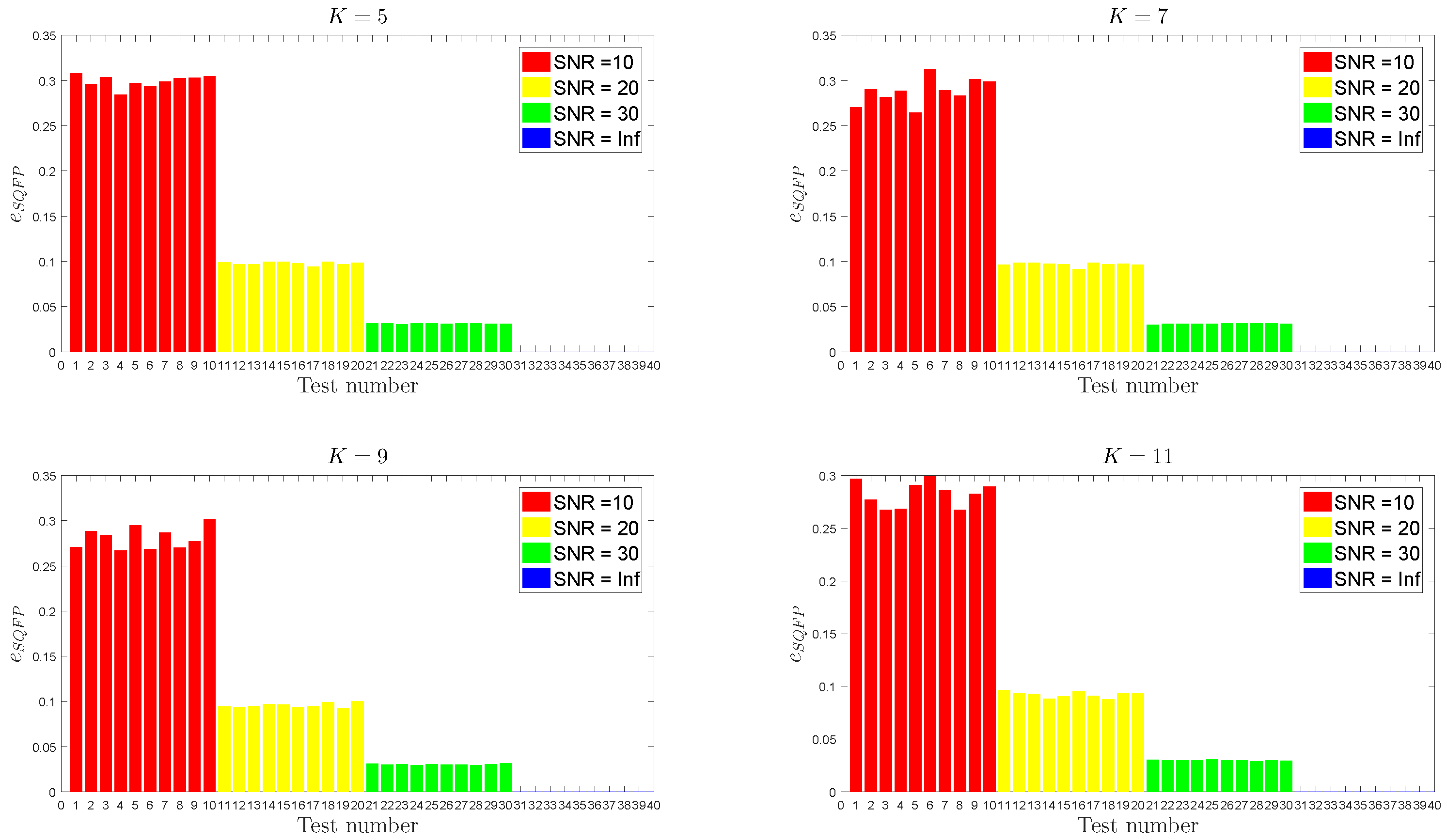
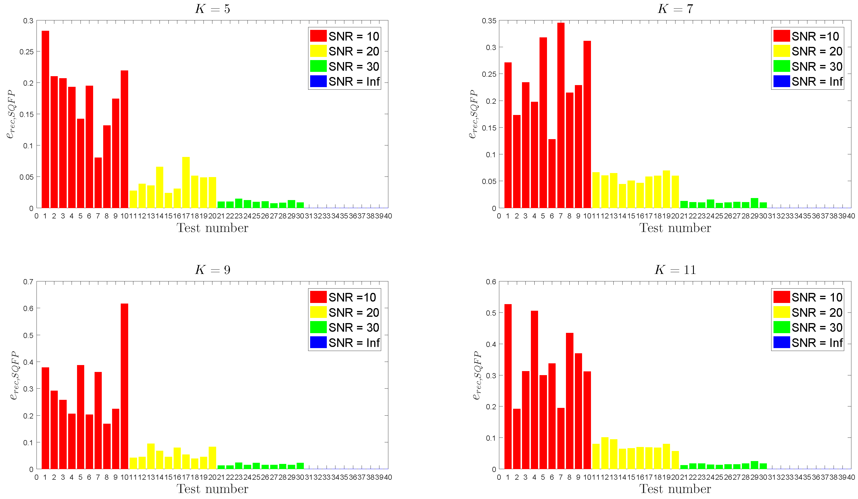
An example of relative errors (7) is given in Figure 2, where SQFP shows the ability to consistently produce solutions whose errors are at about the SNR level. In the same conditions, the recovery error $\parallel x-x_{\mathrm{true}}\parallel /\parallel x_{\mathrm{true}}\parallel$ has the values shown in Figure 3; although with more variability, the errors decrease nicely with the SNR for all values of K.

Figure 2. Relative errors for Sparse Quadratic Feasibility Pump (SQFP) for matrix conditioning of 10,000.

Figure 3. Recovery errors for SQFP for matrix conditioning of 10,000.

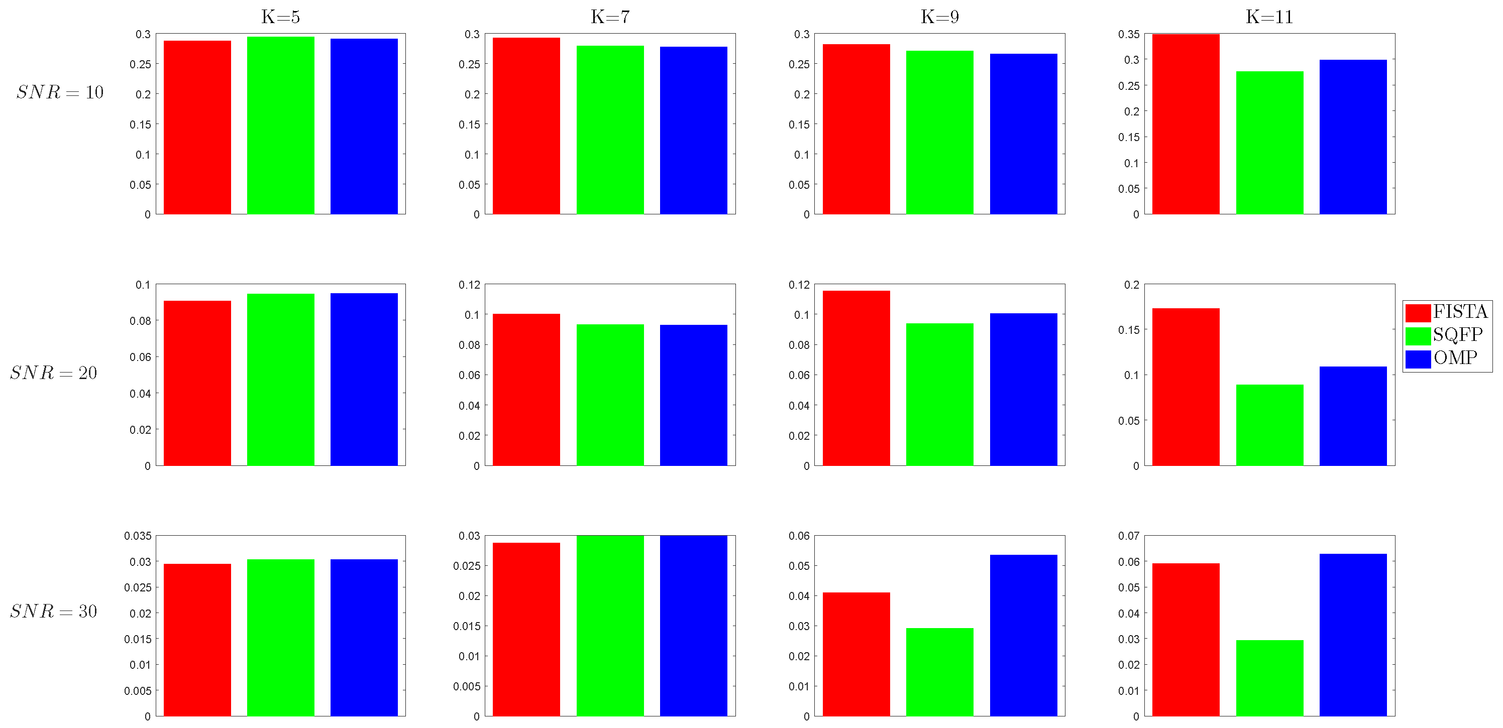
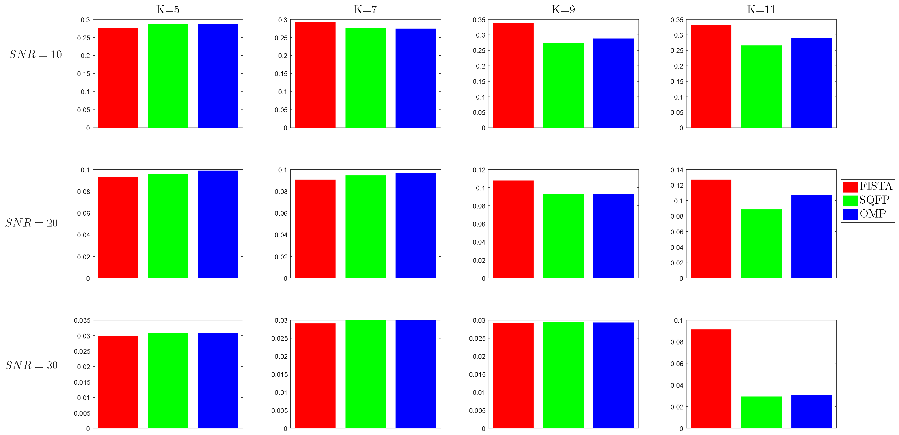
The mean errors obtained by running the tests are displayed in Figure 4, Figure 5, Figure 6 and Figure 7. The first (red) bar in each cell corresponds to the relative error of FISTA, the second (green) is for SQFP and the last (blue) is for OMP.

Figure 4. Mean errors for all algorithms, dictionary size $80\times 200$, condition number 100.

Figure 5. Mean errors for all algorithms, dictionary size $80\times 200$, condition number 1000.

Figure 6. Mean errors for all algorithms, dictionary size $80\times 200$, condition number 10,000.

Figure 7. Mean errors for all algorithms, dictionary size $80\times 200$, condition number 100,000.

It can be seen that as the sparsity level K increases, the SQFP algorithm has a much smaller representation error than FISTA and, only for some condition numbers, than OMP. For $K=5$ and $K=7$, the difference between the algorithms is very small. For larger K, SQFP is clearly better.

To evaluate the complexity of the algorithms, we note that the mean number of iterations is 43.33 for SQFP and 726.56 for FISTA. The FISTA iterations are much less complex and time consuming. The average running time for SQFP is 1.09 s, for FISTA is 0.43 s and for OMP is 0.0025 s.

To evaluate the quality of support recovery, we note that, out of the 640 tests, false negatives appear in 254 (39%) cases for OMP, in 225 (35%) cases for SQFP and in 281 (44%) cases for FISTA. While SQFP needs the longest running time, it recovers the support more precisely than the two other methods. FISTA shows a false positive in 609 (95%) cases. False negatives indicate when an atom is missing from the support of the true solution. False positives appear when the support of the computed solution contains atoms outside the true support.

The second experiment is made with the same parameters as before, but now the dictionary size is $80\times 400$, the condition number is 1000 and $K\in \{9,11,13,15\}$. The overcompleteness factor is larger than in the first experiment, hence the properties of the dictionary are less favorable to sparse recovery. Also, higher sparsity levels are considered, hence the problem becomes more difficult. The mean errors are shown in Figure 8. Now the results of SQFP are even clearly better than those of OMP and FISTA, confirming its ability to work well in more difficult conditions.

Figure 8. Mean errors for all algorithms, dictionary size $80\times 400$, condition number 1000.

4. Conclusions

In this paper we have presented a version of the Feasibility Pump algorithm adapted for the sparse representation problem with $l_2$ norm of the error. Our tests show that the Feasibility Pump gives a better solution when compared with FISTA and OMP, especially at higher sparsity levels. The addition of the weight term for the error proves to be a very important factor for the performance of the algorithm, as it forces the representation error to be smaller. The regularization and the big-M trick limit the magnitude of the values of the coefficients and thus allow the use of this algorithm for ill-conditioned problems. Future lines of research will focus on improving the randomization step, using different regularization terms, treating other norms of the error, implementing recent modifications of FP, like those from [5,9], and adapting the algorithm for other sparse problems reformulations and dictionary learning.