Abstract
Optical coherence tomography (OCT) is an optical high-resolution imaging technique for ophthalmic diagnosis. In this paper, we take advantages of multi-scale input, multi-scale side output and dual attention mechanism and present an enhanced nested U-Net architecture (MDAN-UNet), a new powerful fully convolutional network for automatic end-to-end segmentation of OCT images. We have evaluated two versions of MDAN-UNet (MDAN-UNet-16 and MDAN-UNet-32) on two publicly available benchmark datasets which are the Duke Diabetic Macular Edema (DME) dataset and the RETOUCH dataset, in comparison with other state-of-the-art segmentation methods. Our experiment demonstrates that MDAN-UNet-32 achieved the best performance, followed by MDAN-UNet-16 with smaller parameter, for multi-layer segmentation and multi-fluid segmentation respectively.
1. Introduction
Optical coherence tomography (OCT) is a high-resolution three-dimensional imaging technique, which has significant advantages such as high speed, real time, and non-invasiveness [1]. OCT is widely used clinically and becomes the gold standard in diagnostic imaging for the leading macular diseases such as Diabetic Macular Edema (DME) and choroidal neovascularization(CNV) [2]. DME, caused by fluid leakage from damaged macular blood vessels, is the most common cause of vision loss in American adults [3]. Ophthalmologists use retinal thickness maps to assess the severity of DME. However, manual segmentation of the cyst area is a time-consuming task and prone to human error [4]. Thus, it is necessary to promote the automatic segmentation method of OCT image, which runs fast and prevents subjective factors.
Since the 2000s, classic machine learning methods have been widely used for tasks related to the retina segmentation [5]. Chiu et al. [6] applied a kernel regression-based method to classify the retinal layer and subsequently used Graph Construction as well as dynamic programming to refine the process. Karri et al. [7] utilized structured random forests to learn specific edges of the retinal layer to enhance Graph Construction. Additionally, he improved the spatial consistency between OCT frames by adding appropriate constraints to the Dynamic Programming paradigm for segmentation. Montuoro et al. [8] proposed an auto-context loop for joint segmentation of retinal layer and fluid.
For any segmentation target, deep learning has got comparable or better results to previous methods of classic machine learning [5]. The full convolutional neural network (FCN) [9] has achieved remarkable results in the field of image segmentation. Ronneberger et al. were inspired by the FCN network and proposed the U-Net [10], which combines deep semantic information and spatial information through encoder blocks, decoder blocks and skip connection. U-Net architectures, having achieved the best results in many medical image segmentation tasks, are widely used in OCT segmentation, such as optic nerve head tissues segmentation [11], drusen segmentation [12], intraretinal cystoid fluid (IRC) segmentation [13], fluid regions segmentation [14], and retinal layers segmentation [15]. Lu et al. [16], achieving the best results in the RETOUCH competition, applied Graph-Cut to perform layer segmentation on OCT images as pre-processing and utilize U-Net to segment 3 types of fluid. Venhuizen et al. [13] used a cascaded U-Net network to segment the OCT fluid region and achieved very good accuracy. Inspired by U-Net, Roy et al. [17] proposed ReLayNet which achieved accurate results in a joint segmentation of seven retina layers and fluid region in pathological OCT scans.
A limitation of U-Net is that the consecutive pooling layers reduce spatial information of the feature to learn higher abstract feature representations [18]. Nevertheless, dense prediction tasks need rich spatial information. CE-Net [18], using the first few layers of the pre-trained resnet-34 [19] model based on the ImageNet data set [20] as the network encoder part and applying the decoder part they proposed, have achieved good results in OCT layer segmentation, cell boundary segmentation and lung segmentation. Zhou et al. [21] improved the U-Net and proposed a nested U-Net network (U-Net++) structure to take advantage of deep supervision [22] and re-designed skip pathways which aim at reducing the difference in semantic information between the encoder and decoder blocks. Additionally, a lot of mechanisms have been utilized to segmentation tasks. The multi-scale input, aiming at achieving multiple level sizes of receptive field, has been demonstrated to improve the performance of segmentation network [23,24]. Side output mechanism, first proposed by [25], helps to resolve gradient vanishing problem and capture multi-level representations. Attention mechanism, widely applied in many tasks [26,27,28,29], is able to capture long-range dependencies. In addition, Fu et al. [30] proposed Position Attention Module (PAM) and Channel Attention Module (CAM) to capture global information in spatial and channel dimension respectively.
In this paper, we integrated multi-scale input, multi-scale side output and attention mechanism into our method and present MDAN-UNet, an enhanced nested U-Net architecture for segmentation of OCT images. The main contributions can be listed as:
- We present an enhanced nested U-Net architecture named MDAN-UNet, taking advantages of re-designed skip pathways [21], multi-scale input, multi-scale side output and attention mechanism;
- We propose two versions of our method, which are MDAN-UNet-16 and MDAN-UNet-32 where 16 and 32 denote the number of convolutional kernels in the first encoder block. We validate the proposed methods on two OCT segmentation tasks (layer segmentation and fluid segmentation), and our methods outperform state-of-the-art networks, including Unet++ [21].
2. The Proposed Approach
In order to automatically segment fluid region or layer, we designed a UNet++ [21] alike network. The architecture of our network is shown in Figure 1. As shown in Figure 1, we propose MDAN-UNet, an end-to-end multi-scale and dual attention-enhanced nested U-Net shape architecture. MDAN-UNet consists of three main components, namely multi-scale input, Nested U-Net [21] shape convolutional network as the main body structure and multi-scale side output and multi-scale label.
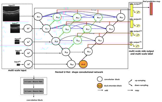
Figure 1.
An overview of the proposed MDAN-UNet architecture. The blue and green parts denote re-designed skip pathways [21] and red line indicates deep supervision.
2.1. Multi-Scale Input
As opposed to [23,24], which constructed multi-scale input by employing average pooling layer, we constructed multi-scale input by taking the first value (in the upper left corner) for every 2 × 2, 4 × 4, 8 × 8 and 16 ×16 non-overlapping area, respectively. We take the way to construct in Figure 1 as an example. Different from max pooling layer with stride equal to 2 by getting max values for every 2 × 2 non-overlapping area, we take the first value(in the upper left corner) for every 2 × 2 non-overlapping area. The way we construct is shown in Figure 2.
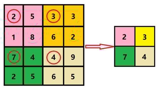
Figure 2.
Illustration of how to construct . We take the first value indicated by the red circle (in the upper left corner) for every 2 × 2 non-overlapping area.
After experiencing a convolution block, the feature maps of current input are simply added to the encoder layers. Let denote the output of node . denotes the input in the i down-sampling layer along the encoder, and denotes the output of node . The formulation of and can be calculated as:
where is the convolution block shown in Figure 1, consisting of two identical operations, for each operation including convolution layer with kernel size 3 × 3, batch normalization, ReLU layer in sequence. Moreover, denotes the down-sampling operation which is a max pooling layer with stride equal to 2. The main advantage of our multi-scale input is: it can achieve multiple level sizes of receptive field so that it can enhance the ability of multi-scale detection; more specifically, it can effectively strengthen the ability of multi-scale lesion segmentation.
2.2. Nested U-Net shape convolutional network
We applied the nested U-Net [21] convolutional network as the main body structure to learn rich representations in the OCT images. Similarly to original nested U-Net, our method comprises an encoder and decoder connected by a series of nested dense convolutions block. As shown in Figure 1, node , identical to [21], denotes the convolution layer of dense block, where i is the down-sampling layer along the encoder and j is the convolution layer of the dense block along the skip pathway.
As opposed to U-Net++ [21] utilizing 2D bilinear up-sampling operation, we apply a 2D transposed convolution operation [31] for up-sampling layer. In addition, we apply dual attention block for the output of node to capture information in global view. Taking model’s parameters into consideration, we construct dual attention block by applying Position Attention Module (PAM) and Channel Attention Module (CAM) [30] at the deepest stage of encoding. Let X be the feature map, our dual attention block can be formulated as:
where denotes a dropout layer [32,33] with rate equal to 0.1 followed by a convolution operation, denotes convolution layer, batch normalization layer and ReLU layer in sequence, and and denote the Position Attention Module and Channel Attention Module respectively whose detail can be found in [30]. Additionally, is the concatenation layer. The architecture of dual attention block is shown in Figure 3.
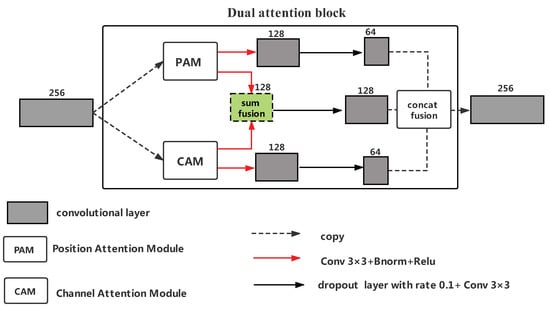
Figure 3.
An overview of the proposed dual attention block in MDAN-UNet-16. The dual attention block in MDAN-UNet-32 has double number of feature maps’ channels for every convolutional layer.
2.3. Multi-Scale Side Output and Multi-Scale Label
We apply multi-scale side output and multi-scale label to help the early layer do back propagation and to relieve gradient vanishing problem. We construct side output by being averaged by multiple convolution layer of dense block along current down-sampling layer. Additionally, we employ to help early training, but only apply as the final prediction map. Let denote the side output computed by the down-sampling layer with index i along the encoder, and it is computed as:
where is a convolution operation with 1*1 kernel.
Owing to multi-scale side output, we construct multi-scale label in the same way as constructing multi-scale input. Precisely, we take the first value(in the upper left corner) for every 2 × 2, 4 × 4 and 8 × 8 non-overlapping area respectively in the original label to get different size of labels for , and respectively. As shown in Figure 1, the total loss in the training stage is:
where is the loss for and the way to calculate is shown in Section 3 below.
3. Loss Function
Our proposed network is trained by minimizing a joint loss function defined as below:
where denotes the weighted multi-class cross entropy and denotes the dice loss.
- Weighted multi-class cross entropy, commonly used in semantic segmentation [9,10,17] to deal with the unbalance classes. Given a pixel i in the image , its formulation can be defined as follow:where denotes the weight associated with pixel i, and C is the number of classes. is the estimated probability of pixel i belonging to class c, and is one for the ground truth of pixel i belonging to class c and zero for others.Because most of the images are backgrounds, the classes are unbalance. What’s more, pixels near the boundary region are difficult to identify. So we apply larger weight for pixels belonging to foreground as well as pixels near the boundary region. Let a pixel i in the image , the formulation of is defined as follow:where is an indicator function, with one for is true and zero for others, and is value of pixel i in the ground map. L represents the values for foreground classes. ∇ denotes the gradient operator.
- Dice loss, proposed by [34], is commonly used to minimize the overlap error between the predicted probability and the true label. It can deal with class imbalance problems. To make sure all pixel values in the predicted probability are positive and in range 0 to 1 when calculating dice loss, we apply soft-max to the predicted probability. The soft-max is defined as:where is the pixel value in feature channel c at the pixel position i. Given a pixel i in the image , the formulation of dice loss is defined as:where is the estimated probability of pixel i in feature channel c. is one for the ground truth of pixel i belonging to class c and zero for others.
4. Experiments
We applied our method on two OCT segmentation tasks: layer segmentation and fluid segmentation. In order to present convincing results in our experiments, we executed all methods three times and averaged the testing values as the results while the train set and test set remained unchanged.
4.1. Experiments settings
The implementation of our network is based on an open-source deep learning toolbox: Pytorch [35]. The experiments were run in Ubuntu 16.04 system with GeForce RTX 2080, which has 8Gigabyte memory. In our experiments, the parameters in Equation (4) are set as . The Adam optimizer [36] is used with initial learning rate of 0.001 for OCT layer segmentation and 0.0005 for OCT fluid segmentation. We adopt a learning rate decay schedule where the current learning rate is multiplied by 0.8 after every 15 epochs. The maximum epoch is 100. For every epoch, we randomly select current batches to train with a probability of 0.8 for OCT layer segmentation and 0.5 for OCT fluid segmentation. In addition, selected batches are randomly cropped so as to increase the robustness of the network. In order to apply fair comparison, the experiments settings are kept constant for all comparison methods.
4.2. Layer Segmentation
4.2.1. Dataset
To show that our method is applicable to OCT multi-layer segmentation, we apply our method to segment 7 retina layers on Duke publicly available data set [6]. Duke publicly available data set [6] comprises 10 DME volumes, each contains 61 SD-OCT B-scan images with a size of 496 × 768. Only 11 images in each volume were labeled by two experts. Eight boundaries were demarcated to divide each B-scan image into nine parts. They include Region above the retina (RaR), Inner limiting membrane (ILM), Nerve fiber ending to Inner plexiform layer(NFL-IPL), Inner Nuclear layer (INL), Outer plexiform layer (OPL), Outer Nuclear layer to Inner segment myeloid (ONL-ISM), Inner segment ellipsoid (ISE), Outer segment to Retinal pigment epithelium (OS-RPE) and Region below the retina (RbR).
4.2.2. Preprocessing
The way we processed the dataset is nearly identical to [7]. Firstly, we picked 110 OCT images with labelled and all the “nan” in contour was interpolated by the intermediate location value. Then, the two contour locations provided by two experts were averaged for 55 images from the first five volumes as train data annotation. We evaluated methods respectively on both annotations from two experts for the rest 55 images. Due to the lack of expert edge locations, we only chose the dataset with columns from 120 to 650. To train in the U-Net shape network, rows from input images were zero-padded to size of 496 × 544 and rows from labels were padded with −1 to size of 496 × 544. When calculating the loss or evaluation metrics, the value of −1 is ignored. Due to the small number of training samples are available, we applied three processes of data argumentation to enhance the robustness as well as invariance properties of the network and preventing from overfitting, namely random horizontal flip, resizing after random cropping and elastic deformation [37].
4.2.3. Comparative Methods and Metric
We compared our proposed method with some state-of-the-art OCT layer segmentation algorithms: learning layer specific edges method (LSE) [7], U-Net [10], ReLayNet [17], CE-Net [18] and U-Net++ with deep supervision [21]. Note that we did not run LSE [7] in out experiment and apply the original result in [7] due to the fact that the way we processed the data set is nearly identical to [7]. To evaluate the performance, we adopted three standard metrics as calculated in [6,7]. They are dice score (denote it as DSC), estimated contour error for each layer (denote it as CE) and estimated thickness error for each layer (denote it as TE).
- Dice score, which has been commonly used to evaluate the overlap of OCT segmentation:where P and Y are predicted output and ground truth respectively.
- Estimated contour error calculates mean absolute difference between the predicted layer contour and the ground truth layer contour along the column. The estimated contour error for contour c can be formulated aswhere and denote the predicted row location of contour c in column i and the ground truth one respectively, and N is the number of pixels for one row.
- Estimated thickness error for each layer calculates absolute difference in layer thickness. The estimated thickness error for layer l can be formulated as:where and denote the number of pixels belonging to layer l in column i and the ground truth one respectively. N is the number of pixels for one row.
4.2.4. Results
a. Qualitative evaluation
We present a qualitative evaluation of two versions of MDAN-UNet in contrast with the comparative methods. We observe that three comparative methods perform well at layer segmentation but poorly at background segmentation (as indicated by the red arrows in Figure 4). U-Net shows the worst performance, followed by U-Net++ and CE-Net, for misdivision of background region into layer region. Due to the fact that there is no attention mechanism on comparative methods, comparative methods have a lot of false detections in the background region except ReLayNet. ReLayNet, using larger convolutional kernel whose size is 7 × 3, has a larger receptive field and therefore achieves a relatively good performance in terms of segmentation of background region compared with U-Net, U-Net++ and CE-Net. The prediction of MDAN-UNet-32, MDAN-UNet-16 and ReLayNet are of high quality and outperform other methods.
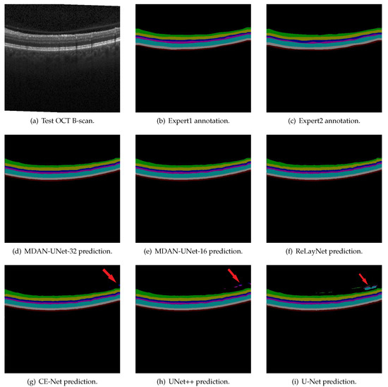
Figure 4.
Layer segmentation comparison of a Test OCT B-scan. (a) A Test OCT B-scan, (b,c) the segmentation results completes by two different experts, (d) MDAN-UNet-32 prediction, (e) MDAN-UNet-16 prediction, (f–i) comparative methods’ predictions
b. Quantitative evaluation
We present quantitative evaluation of two versions of MDAN-UNet in contrast with the comparative methods in terms of the number of parameters and convolutional kernels (Table 1), mean dice score (Table 2), mean thickness error for each layer (Table 3) and mean contour error (Table 4).

Table 1.
Comparison of the number of networks’ parameters and convolutional kernels. in column headers refer to encoder/decoder and the values in those columns denote the number of convolutional kernels.
Table 2.
Mean dice score(DSC): performance comparison of layer segmentation.The best one shown in type and ‘*’ marks the second best.
Table 3.
Thickness error(TE) for each layer: performance comparison of layer segmentation. The best one shown in type and ‘*’ marks the second best.
Table 4.
Mean contour error(CE): performance comparison of layer segmentation. The best one shown in type and ‘*’ marks the second best.
We report the number of parameters and convolutional kernels of models given in Table 1. We observe that the number of parameters of MDAN-UNet-16, which is 3.77M, is much less than others. Additionally, ReLayNet [17], with 7.74 M parameters, has the second smallest parameters among them. MDAN-UNet-32 has about 6M more parameters than UNet++ [21] and about 1.6M more parameters than U-Net [10]. Moreover, CE-Net [18] has the largest parameters.
The dice score of each experiment for every epoch is illustrated in Figure 5. As we can see, all the methods reach an average DSC of 0.8 in the first 20 epochs and achieve stable DSC after 80 epochs. In addition, the DSC for MDAN-UNet-32 increases at a faster rate compared with other methods in the first 10 epochs, and the rapid increase in DSC for MDAN-UNet-32 may be attributed to the multi-scale side output which can enhance deep supervision and help early layer training. The DSC for MDAN-UNet-32, MDAN-UNet-16 and CE-Net [18] maintain a relatively stable growth after 15 epochs, while the DSC for U-Net [10], UNet++ [21] and ReLayNet [17] fluctuates. The DSC for MDAN-UNet is more stable than the DSC for U-Net [10], UNet++ [21] and ReLayNet [17], and the possible reasons can be listed as follows: in the first place, MDAN-UNet takes advantages of multi-scale input which could achieve multiple level sizes of receptive field; secondly, MDAN-UNet utilizes multi-scale side output and multi-scale label which could help layer training correctly; moreover, MDAN-UNet applies dual attention block to capture global information in a spatial and channel dimension.
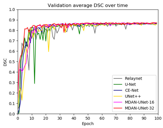
Figure 5.
Evolution of test dice score (DSC) when training on Duke publicly available dataset. The DSC is the average of DSC for expert 1 annotation and expert 2 annotation.
From the comparison shown in Table 2, Table 3 and Table 4, MDAN-UNet-32 achieves best performance to achieve the highest average dice score: 0.883 for expert 1 annotation and 0.866 for expert 2 annotation, lowest average thickness error(TE): 1.514 and 1.745 for two experts’ annotation respectively, and lowest average contour error: 1.193 and 1.362 for two experts’ annotation respectively. From the aspect of average dice score, average thickness error and average contour error, MDAN-UNet-16 achieves second best performance, followed by U-Net++, CE-Net, U-Net, ReLayNet and LSE in sequence. With the smallest parameter, MDAN-UNet-16 shows promising performance and outperforms U-Net++, CE-Net, ReLayNet and LSE in layer segmentation. From the aspect of average dice score and average thickness error, all fully convolution networks outperform LSE, the traditional segmentation method. When it comes to contour error(CE), LSE achieves an average of 1.369 for expert 1 annotation, the same as U-Net, and achieve an average of 1.463 for expert 2 annotation which is better than U-Net with an average of 1.521.
c. Ablation study
In order to demonstrate the effectiveness of multi-scale input, multi-scale side output and the dual attention block, we conducted the following ablation experiments. Our proposed method is an enhanced UNet++ network; therefore, UNet++ [21] is the most fundamental baseline model. We replace 2D transposed convolution with 2D bilinear up-sampling operation in UNet++ [21], and called the modified UNet++ as Backbone. Additionally, we add dual attention block to Backbone (remove , , , , , and from MDAN-UNet-32, as shown in Figure 1 while others remain unchanged), and denote it as Backbone+Attention Block. We remove multi-scale side output and multi-scale label (remove , , , and let as total loss shown in Figure 1) from MDAN-UNet-32 while others remain unchanged, and denote it as Backbone+Attention Block+Multi-input.
As shown in Table 5, we observe that Backbone shows a slight improvement in performance in comparison of UNet++ [21], and that Backbone+Attention Block shows better performance than Backbone except for the average of thickness error(TE), which verifies the effectiveness of the dual attention block. We also observe that Backbone+Attention Block+Multi-input shows better performance than Backbone+Attention Block in all aspects, so the multi-scale input could improve the performance. In addition, Backbone+Attention Block+Multi-input yields a result of 0.883 in average dice score for expert 1 annotation, the same as MDAN-UNet-32 (Backbone+Attention Block+Multi-input+Multi-scale side output and Multi-scale label) yields, but performs poorly in other aspects. In other words, multi-scale side output and multi-scale label could further improve the performance. From the above analysis, we can draw a conclusion that multi-scale input, multi-scale side output and the dual attention block improve the performance, respectively.
Table 5.
Ablation study on Duke publicly available dataset. The value is an average of DSC, TE or CE. The best one shown in type.
4.3. Fluid Segmentation
4.3.1. Datasets
In this paper, we also showed that our method is applicable for OCT multi-fluid segmentation. We applied our method to segment 3 types of retinal fluid. The datasets used in this paper were kindly provided by the MICCAI RETOUCH Group [38]. There are a total of 112 volumes (70 volumes for the training set and 42 volumes for the test set) with three different types of fluid manually labeled: the intraretinal fluid (IRF), subretinal fluid(SRF) and the pigment epithelial detachment (PED). For the training set, 24 volumes were acquired with each of the two OCT images devices: Cirrus, Spectralis. The remaining 22 volumes were acquired with Topcon (T-1000 and T-2000). OCT acquired with Cirrus comprises 128 B-scan images with a size of 512 × 1024 and OCT acquired with Spectralis comprises 49 B-scan images with a size of 512 × 496. OCT acquired with Topcon comprises 128 B-scan images with a size of 512 × 650 (T-1000) or 512 × 885 (T-2000). Due to the fact that the segmentation maps of test set were kept secret, we evaluated our method on the training set by dividing them into our own training set and test set under the approval of the MICCAI RETOUCH Group [38]. Precisely, we chose the first 15, 15 and 14 volumes acquired with Cirrus, Spectralis and Topcon respectively as our training set in this paper. The last 9, 9 and 8 volumes acquired with Cirrus, Spectralis and Topcon, respectively, were used to be our test set. In a word, we had 44 volumes for the training set and 26 volumes for the test set.
4.3.2. Preprocessing
The way we processed the dataset is similar to [39]. Because of the variations between images acquired with different devices, we normalized the voxel values to range [0,255] by histogram matching using a randomly selected OCT scan as the template. In addition, a median filter along the z-dimension was applied to reduce noise. In order to utilize the 3D information, each training image was obtained by concatenating three adjacent slices in a sequence. Due to the different sizes of the images, slices in the training set were cropped to a size of 512 × 400 by putting the fluid region in the center of the y-dimension. Thus, the size of each image in the training set is 512 × 400 × 3 pixels. For the test set, we applied networks to test OCT from different devices respectively so that we don’t have to apply the cropping process. Notes that OCT images acquired with Topcon are zero-padded from a size of 512 × 650 × 3 pixels or 512 × 885 × 3 pixels to 512 × 896 × 3 pixels and labels are padded with −1, which is ignored when calculating evaluation metrics.
4.3.3. Comparative Methods and Metric
We compare our proposed method with some state-of-the-art deep FCN algorithms: U-Net [10] and U-Net++ with deep supervision [21]. To evaluate the performance, we adopt 2 standard metrics suggested by [39]. They are dice score (denote it as DSC) and absolute volume difference (AVD), where the formulation of dice score have been defined above.
- Absolute volume difference (AVD) :where P and Y are predicted output and ground truth respectively.
4.3.4. Results
a. Qualitative evaluation
We present a qualitative evaluation for fluid segmentation. As shown in Figure 6, we observe that UNet++ and U-Net relatively has a large number of missed detections of IRF (green region). In addition, U-Net prediction shows a large number of false detections of SRF (yellow region) and other networks perform well on the segmentation of SRF. We also observe that the prediction of MDAN-UNet-32 is of high quality and outperforms other methods. MDAN-UNet-16 prediction outperforms UNet++ and U-Net for less missed detections for IRF. Noted that there are still a lot of miss detections of PED (red region) for MDAN-UNet-16 and a lot of false detections of PED for U-Net and UNet++. The high imbalance of classes may partly explain why it is difficult for automatic segmentation methods to segment fluid correctly.
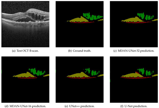
Figure 6.
Fluid segmentation comparison of a Test OCT B-scan from Spectralis. The green region indicates IRF, the yellow region refers to SRF and the red part refers to PED.
b. Quantitative evaluation
We present quantitative evaluation MDAN-UNet-16 and MDAN-UNet-32 in contrast with the comparative methods in terms of mean dice score and mean AVD [mm].
From the comparison shown in Table 6, we observe that the segmentation of IRF is better than for SRF and PED. However, [38] reported that the segmentation of PED is better than for SRF and IRF. Additionally, automatic methods’ performance on Topcon scans is the lowest and [38] reports that automatic method performance on Spectralis scans is the lowest. The factor that we evaluate our method on the training set by dividing them into our own training set and test set may partly explain why there are some differences between us and [38]. We also observe that MDAN-UNet-32 achieves the best average dice score: 0.677 for images from Cirrus, 0.685 for images from Spectralis and 0.648 for images from Topcon, followed by MDAN-UNet-16 with an average dice score of 0.662, 0.679 and 0.609 for images from Cirrus, Spectralis and Topcon respectively. For the images from Cirrus, U-Net achieves a mean dice score of 0.627 for all, which is better than UNet++. Nevertheless, UNet++ shows a better performance than U-Net in terms of mean dice score for the images from Spectralis and Topcon. From the aspect of average dice score, MDAN-UNet-16 and MDAN-UNet-32 always achieve top two performances. In addition, UNet++ outperforms U-Net in Cirrus and Topcon images but gets worst performance in Spectralis images.
Table 6.
Mean dice score (standard deviation): performance comparison of fluid segmentation. The best one shown in type and ‘*’ marks the second best.
We also present performance comparison of fluid segmentation in terms of mean AVD [mm] in Table 7. We observe that MDAN-UNet-32 achieves the lowest mean AVD for images from three types of devices. MDAN-UNet-16 ranks second in terms of mean AVD for images from Spectralis and Topcon. For images from Cirrus, U-Net achieves a mean AVD of 0.161 and outperforms MDAN-UNet-16 and UNet++. Thus, in terms of average dice score and mean AVD, MDAN-UNet-32 performs best, and MDAN-UNet-16 is the second.
Table 7.
Mean AVD [mm] (standard deviation): performance comparison of fluid segmentation. The best one shown in type and ‘*’ marks the second best.
4.4. Discussion
Our experiment demonstrates that MDAN-UNet-32 and MDAN-UNet-16 outperform the state-of-the-art methods in terms of retinal layer segmentation and fluid segmentation. We observe that the performance of fluid segmentation methods varies for OCT from different devices. There are two possible reasons for this. In the first place, each OCT volume in the RETOUCH dataset [38] corresponds to different patients, and the size and number of fluid lesions in different OCT volumes are different. For example, some OCT volumes only have a single small volume of fluid, while some OCT volumes have three kinds of fluids with large region. Therefore, the data distributions in OCT volume collected by the three devices are not consistent. Secondly, the resolutions of OCT volume from the three devices are also different. For example, an OCT volume for Circus, Spectralis and Topcon consists of 128 B-scans with a size of 512 × 1024, 49 B-scans with a size of 512 × 496 and 128 B-scans with a size of 512 × 885 pixels(T-2000) or 512 × 650(T-1000) respectively. In addition, the axial resolutions of OCT for Circus, Spectralis and Topcon are 2 m, 3.9 m and 2.6/3.5 m (T-2000/T-1000) respectively [38].
We also observe that MDAN-UNet significantly outperforms comparative methods in fluid segmentation but provides marginal improvements in layer segmentation. There are some possible reasons responsible for inconsistency of the results. The first possible reason is that the position of each layer is relatively fixed while the position of each fluid varies greatly, and the distribution of layers is similar between OCT volumes while the distribution of fluids varies greatly between OCT volumes. The second possible reason is that the layer region accounts for a large proportion of the OCT images so that slight false detections or missed detections have little effect on the result while the fluid region is usually small so that slight false detections or missed detections will have a great impact on the results. The significant improvement of the performance of the proposed algorithm for fluid segmentation verifies the effectiveness of the proposed multi-scale input, multi-scale side output and dual attention mechanism for lesion segmentation of OCT.
5. Conclusions
In this paper, we propose an end-to-end multi-scale nested U-Net shape deep network to segment seven retina layers and three types of fluid respectively. The proposed architecture takes advantages of multi-scale input, multi-scale side output, re-designed skip pathways from U-Net++ [21] and dual attention mechanism. The multi-scale input aims at enabling the network to fuse multi-scale information, and multi-scale side output aims at enhancing the early layer training and deep supervision. In addition, re-designed skip pathways reduce the information gap between encoder blocks and decoder blocks, and dual attention block enables capturing global information in spatial and channel dimension respectively. We proposed MDAN-UNet-16, the small network, and MDAN-UNet-32, the big one. MDAN-UNet-32 outperforms the state-of-the-art retinal layer and fluid segmentation methods and MDAN-UNet-16, with the smallest parameters, achieves a better performance than LSE [7], U-Net [10], ReLayNet [17], CE-Net [18] and U-Net++ with deep supervision [21].
Author Contributions
Conceptualization, Y.S. and Q.J.; Data curation, W.L.; Formal analysis, W.L. and Y.S.; Funding acquisition, Y.S. and Q.J.; Investigation, W.L.; Methodology, W.L.; Project administration, Y.S.; Software, W.L.; Writing—original draft, W.L.; Writing—review & editing, Y.S. and Q.J. All authors have read and agreed to the published version of the manuscript.
Funding
This work was supported by the National Natural Science Foundation of China under Grant No. 61671272 and by the Opening Project of Guangdong Province Key Laboratory of Big Data Analysis and Processing under Grant No. 201803.
Conflicts of Interest
The authors declare no conflict of interest.
References
- Huang, D.; Swanson, E.A.; Lin, C.P.; Schuman, J.S.; Stinson, W.G.; Chang, W.; Hee, M.R.; Flotte, T.; Gregory, K.; Puliafito, C.A.; et al. Optical coherence tomography. Science 1991, 254, 1178–1181. [Google Scholar] [CrossRef] [PubMed]
- Schmidt-Erfurth, U.; Waldstein, S.M. A paradigm shift in imaging biomarkers in neovascular age-related macular degeneration. Prog. Retin. Eye Res. 2016, 50, 1–24. [Google Scholar] [CrossRef] [PubMed]
- Davidson, J.A.; Ciulla, T.A.; McGill, J.B.; Kles, K.A.; Anderson, P.W. How the diabetic eye loses vision. Endocrine 2007, 32, 107–116. [Google Scholar] [CrossRef] [PubMed]
- DeBuc, D.C. A review of algorithms for segmentation of retinal image data using optical coherence tomography. Image Segm. 2011, 1, 15–54. [Google Scholar]
- Schmidt-Erfurth, U.; Sadeghipour, A.; Gerendas, B.S.; Waldstein, S.M.; Bogunović, H. Artificial intelligence in retina. Prog. Retin. Eye Res. 2018, 67, 1–29. [Google Scholar] [CrossRef]
- Chiu, S.J.; Allingham, M.J.; Mettu, P.S.; Cousins, S.W.; Izatt, J.A.; Farsiu, S. Kernel regression based segmentation of optical coherence tomography images with diabetic macular edema. Biomed. Opt. Express 2015, 6, 1172–1194. [Google Scholar] [CrossRef]
- Karri, S.; Chakraborthi, D.; Chatterjee, J. Learning layer-specific edges for segmenting retinal layers with large deformations. Biomed. Opt. Express 2016, 7, 2888–2901. [Google Scholar] [CrossRef]
- Montuoro, A.; Waldstein, S.M.; Gerendas, B.S.; Schmidt-Erfurth, U.; Bogunović, H. Joint retinal layer and fluid segmentation in OCT scans of eyes with severe macular edema using unsupervised representation and auto-context. Biomed. Opt. Express 2017, 8, 1874–1888. [Google Scholar] [CrossRef]
- Long, J.; Shelhamer, E.; Darrell, T. Fully convolutional networks for semantic segmentation. In Proceedings of the IEEE Conference on Computer Vision and Pattern Recognition, Boston, MA, USA, 7–12 June 2015; pp. 3431–3440. [Google Scholar]
- Ronneberger, O.; Fischer, P.; Brox, T. U-net: Convolutional networks for biomedical image segmentation. In Proceedings of the International Conference on Medical Image Computing and Computer-Assisted Intervention, Munich, Germany, 5–9 October 2015; pp. 234–241. [Google Scholar]
- Devalla, S.K.; Renukanand, P.K.; Sreedhar, B.K.; Perera, S.; Mari, J.M.; Chin, K.S.; Tun, T.A.; Strouthidis, N.G.; Aung, T.; Thiéry, A.H.; et al. DRUNET: A dilated-residual u-net deep learning network to digitally stain optic nerve head tissues in optical coherence tomography images. arXiv 2018, arXiv:1803.00232. [Google Scholar] [CrossRef]
- Zadeh, S.G.; Wintergerst, M.W.; Wiens, V.; Thiele, S.; Holz, F.G.; Finger, R.P.; Schultz, T. CNNs enable accurate and fast segmentation of drusen in optical coherence tomography. In Deep Learning in Medical Image Analysis and Multimodal Learning for Clinical Decision Support; Springer: New York, NY, USA, 2017; pp. 65–73. [Google Scholar]
- Venhuizen, F.G.; van Ginneken, B.; Liefers, B.; van Asten, F.; Schreur, V.; Fauser, S.; Hoyng, C.; Theelen, T.; Sánchez, C.I. Deep learning approach for the detection and quantification of intraretinal cystoid fluid in multivendor optical coherence tomography. Biomed. Opt. Express 2018, 9, 1545–1569. [Google Scholar] [CrossRef]
- Chen, Z.; Li, D.; Shen, H.; Mo, H.; Zeng, Z.; Wei, H. Automated segmentation of fluid regions in optical coherence tomography B-scan images of age-related macular degeneration. Opt. Laser Technol. 2020, 122, 105830. [Google Scholar] [CrossRef]
- Ben-Cohen, A.; Mark, D.; Kovler, I.; Zur, D.; Barak, A.; Iglicki, M.; Soferman, R. Retinal layers segmentation using fully convolutional network in OCT images. 2017. Available online: https://www.rsipvision.com/wp-content/uploads/2017/06/Retinal-Layers-Segmentation.pdf (accessed on 29 February 2020).
- Lu, D.; Heisler, M.; Lee, S.; Ding, G.W.; Navajas, E.; Sarunic, M.V.; Beg, M.F. Deep-learning based multiclass retinal fluid segmentation and detection in optical coherence tomography images using a fully convolutional neural network. Med Image Anal. 2019, 54, 100–110. [Google Scholar] [CrossRef] [PubMed]
- Roy, A.G.; Conjeti, S.; Karri, S.P.K.; Sheet, D.; Katouzian, A.; Wachinger, C.; Navab, N. ReLayNet: Retinal layer and fluid segmentation of macular optical coherence tomography using fully convolutional networks. Biomed. Opt. Express 2017, 8, 3627–3642. [Google Scholar] [CrossRef] [PubMed]
- Gu, Z.; Cheng, J.; Fu, H.; Zhou, K.; Hao, H.; Zhao, Y.; Zhang, T.; Gao, S.; Liu, J. CE-Net: Context encoder network for 2D medical image segmentation. IEEE Trans. Med Imaging 2019, 38, 2281–2292. [Google Scholar] [CrossRef]
- He, K.; Zhang, X.; Ren, S.; Sun, J. Deep residual learning for image recognition. In Proceedings of the IEEE Conference on Computer Vision and Pattern Recognition, Las Vegas, NV, USA, 27–30 June 2016; pp. 770–778. [Google Scholar]
- Deng, J.; Dong, W.; Socher, R.; Li, L.J.; Li, K.; Fei-Fei, L. Imagenet: A large-scale hierarchical image database. In Proceedings of the 2009 IEEE Conference on Computer Vision and Pattern Recognition, Miami, FL, USA, 20–25 June 2009; pp. 248–255. [Google Scholar]
- Zhou, Z.; Siddiquee, M.M.R.; Tajbakhsh, N.; Liang, J. Unet++: A nested u-net architecture for medical image segmentation. In Deep Learning in Medical Image Analysis and Multimodal Learning for Clinical Decision Support; Springer: New York, NY, USA, 2018; pp. 3–11. [Google Scholar]
- Lee, C.-Y.; Xie, S.; Gallagher, P.; Zhang, Z.; Tu, Z. Deeply-supervised nets. In Proceedings of the 18th International Conference on Artificial Intelligence and Statistics, San Diego, CA, USA, 9–12 May 2015; Volume 38, pp. 562–570. [Google Scholar]
- Fu, H.; Cheng, J.; Xu, Y.; Wong, D.W.K.; Liu, J.; Cao, X. Joint optic disc and cup segmentation based on multi-label deep network and polar transformation. IEEE Trans. Med Imaging 2018, 37, 1597–1605. [Google Scholar] [CrossRef]
- Abraham, N.; Khan, N.M. A novel focal tversky loss function with improved attention u-net for lesion segmentation. In Proceedings of the 2019 IEEE 16th International Symposium on Biomedical Imaging (ISBI 2019), Venice, Italy, 8–11 April 2019; pp. 683–687. [Google Scholar]
- Xie, S.; Tu, Z. Holistically-nested edge detection. In Proceedings of the IEEE International Conference on Computer Vision, Santiago, Chile, 11–18 December 2015; pp. 1395–1403. [Google Scholar]
- Chu, X.; Yang, W.; Ouyang, W.; Ma, C.; Yuille, A.L.; Wang, X. Multi-context attention for human pose estimation. In Proceedings of the IEEE Conference on Computer Vision and Pattern Recognition, Honolulu, HI, USA, 21–26 July 2017; pp. 1831–1840. [Google Scholar]
- Li, H.; Xiong, P.; An, J.; Wang, L. Pyramid attention network for semantic segmentation. arXiv 2018, arXiv:1805.10180. [Google Scholar]
- Oktay, O.; Schlemper, J.; Folgoc, L.L.; Lee, M.; Heinrich, M.; Misawa, K.; Mori, K.; McDonagh, S.; Hammerla, N.Y.; Kainz, B.; et al. Attention u-net: Learning where to look for the pancreas. arXiv 2018, arXiv:1804.03999. [Google Scholar]
- Zhang, P.; Liu, W.; Wang, H.; Lei, Y.; Lu, H. Deep gated attention networks for large-scale street-level scene segmentation. Pattern Recognit. 2019, 88, 702–714. [Google Scholar] [CrossRef]
- Fu, J.; Liu, J.; Tian, H.; Li, Y.; Bao, Y.; Fang, Z.; Lu, H. Dual attention network for scene segmentation. In Proceedings of the IEEE Conference on Computer Vision and Pattern Recognition, Long Beach, CA, USA, 16–20 June 2019; pp. 3146–3154. [Google Scholar]
- Zeiler, M.D.; Krishnan, D.; Taylor, G.W.; Fergus, R. Deconvolutional networks. In Proceedings of the 2010 IEEE Computer Society Conference on Computer Vision and Pattern Recognition, San Francisco, CA, USA, 13–18 June 2010; pp. 2528–2535. [Google Scholar]
- Hinton, G.E.; Srivastava, N.; Krizhevsky, A.; Sutskever, I.; Salakhutdinov, R.R. Improving neural networks by preventing co-adaptation of feature detectors. arXiv 2012, arXiv:1207.0580. [Google Scholar]
- Srivastava, N.; Hinton, G.; Krizhevsky, A.; Sutskever, I.; Salakhutdinov, R. Dropout: A simple way to prevent neural networks from overfitting. J. Mach. Learn. Res. 2014, 15, 1929–1958. [Google Scholar]
- Milletari, F.; Navab, N.; Ahmadi, S.A. V-net: Fully convolutional neural networks for volumetric medical image segmentation. In Proceedings of the 2016 Fourth International Conference on 3D Vision (3DV), Stanford, CA, USA, 25–28 October 2016; pp. 565–571. [Google Scholar]
- Paszke, A.; Gross, S.; Chintala, S.; Chanan, G.; Yang, E.; DeVito, Z.; Lin, Z.; Desmaison, A.; Antiga, L.; Lerer, A. Automatic differentiation in pytorch. 2017. Available online: https://openreview.net/pdf?id=BJJsrmfCZ (accessed on 29 February 2020).
- Kingma, D.P. Adam: A method for stochastic optimization. arXiv 2015, arXiv:1412.6980. [Google Scholar]
- Simard, P.Y.; Steinkraus, D.; Platt, J.C. Best practices for convolutional neural networks applied to visual document analysis. In Proceedings of the 7th International Conference on Document Analysis and Recognition, Edinburgh, UK, 6 August 2003. [Google Scholar]
- Bogunović, H.; Venhuizen, F.; Klimscha, S.; Apostolopoulos, S.; Bab-Hadiashar, A.; Bagci, U.; Beg, M.F.; Bekalo, L.; Chen, Q.; Ciller, C.; et al. RETOUCH: The Retinal OCT Fluid Detection and Segmentation Benchmark and Challenge. IEEE Trans. Med Imaging 2019, 38, 1858–1874. [Google Scholar] [CrossRef] [PubMed]
- Tennakoon, R.; Gostar, A.K.; Hoseinnezhad, R.; Bab-Hadiashar, A. Retinal fluid segmentation and classification in OCT images using adversarial loss based CNN. In Proceedings of the MICCAI Retinal OCT Fluid Challenge (RETOUCH), Quebec, QC, Canada, 10–14 September 2017; pp. 30–37. [Google Scholar]


© 2020 by the authors. Licensee MDPI, Basel, Switzerland. This article is an open access article distributed under the terms and conditions of the Creative Commons Attribution (CC BY) license (http://creativecommons.org/licenses/by/4.0/).