Optimal Model for Carsharing Station Location Based on Multi-Factor Constraints

Abstract

The development of the sharing economy has made carsharing the main future development model of car rental. Carsharing network investment is enormous, but the resource allocation is limited. Therefore, the reasonable location of the carsharing station is important to the development of carsharing companies. On the basis of the current status of carsharing development, this research considers multiple influencing factors of carsharing to meet the maximum user demand. Meanwhile, the constraint of the limited cost of the company is considered to establish a nonlinear integer programming model for station location of carsharing. A genetic algorithm is designed to solve the problem by analyzing the location model of the carsharing network. Finally, the results of a case study of Lanzhou, China show the effectiveness of the establishment and solution of the station location model.

1. Introduction

Carsharing is gaining popularity due to its green advantages. Carsharing helps reduce the number of private cars, which alleviates traffic congestion in turn [1]. Carsharing refers to the leasing business in which cars are owned by a carsharing company and used by different users at varying times with measurement by duration and mileage. Unlike traditional offline car rental service and day-by-day billing units, carsharing users register and authenticate on their mobile phones, use applications to find surrounding stations, and rent cars by time [2]. This research analyzes electric carsharing, which is a carsharing that is powered by electricity and has less pollution impact than traditional cars.

This research focuses on the types of electric carsharing [3,4] in which the cars can be fetched and parked at fix or free stations. Fix stations require a certain area to store cars, and the costs include land rent, charger and station construction costs [5,6]. If the area does not have fix stations, then users can park their cars on the public parking space in a certain area. Different fees of users are charged for parking at varying stations. However, the parking fee is paid by the company. Therefore, for the carsharing company, the free station does not require the cost of station construction, but parking costs will be incurred. The construction of fixed stations is conducive to the management of cars, and free stations are convenient for users to use cars and for reducing the cost of station construction. The combination of two operation forms is conducive to the sustainable development of carsharing.

Carsharing is advantageous because it provides great convenience for users and improves the flexibility of cars [7]. Zhu [8] analyzed the objective conditions of the new energy carsharing in China and revealed the popularization value and prospects of carsharing in China. Feng [9] analyzed the current development status and future scale of the major car long-term rental, short-term rental, and online car rental markets. These studies are biased toward policy and market analysis. Notably, carsharing has a great future in the transportation field. However, the development of the carsharing industry is still in its early stages. The problems of few stations, few available cars, and few chargers have become key restricting factors of the development of carsharing companies [10]. Some studies have found that carsharing network settings can affect user willingness and company development. Ciari [11] used a binary logistic model and showed that the location of stations actually affects potential membership. This research used elastic analysis to find the relationship between distance and number of users but did not introduce specific methods for station location optimization. Correia [12] found that financial losses can be reduced through appropriate choices with respect to the number, location, and size of the depots. This research provided the foundation for the necessity of the station location optimization model.

Scholars have conducted the following research to address the problems of carsharing station location optimization. Jiang [13] used analytic hierarchy process to calculate the best scheme for carsharing stations. The study identified variables with a significant effect on station location selection but did not build an optimization model for carsharing station location determination. Lu [14] used the interval fuzzy soft set method of risk preference for each carsharing station in Wang Cheng County. The evaluation of the plan has certain reference significance for the location and future planning of carsharing. This method is more suitable for evaluating existing carsharing stations than for planning for new cities. The above-mentioned research methods are relatively subjective. Other methods using mathematical models are presented as follows. Çalık [15] illustrated a carsharing locating recharging station model that operates under demand uncertainty. The research developed a demand forecasting method that allows the generation of many demand scenarios. Hu [16] formulated a mixed queuing network model for the joint design of fleet size and station capacities. The optimization problem was solved by the genetic algorithm. They proved that the profit is maximized when the existing road congestion is moderate. This research mainly considered the carsharing model of the fixed station but ignored the setting of free stations. Wielinski, G [17] researched the travel area and behavior of free-floating carsharing users. This study mainly considered the operation model of free-floating carsharing but ignored the setting of fixed stations. Zheng [18] proposed a method for optimizing the location of charging stations for one-way electric carsharing systems. The objective function was to maximize the profit of carsharing service. Simulations were performed to prove the effectiveness of the research method. The final station was optimized by 0–1 variable station selection among existing candidate sites. However, the study failed to provide scientific theoretical basis for the selection of the alternative station. Lee [19] analyzed eight spatial elements related to carsharing location. A model was established to determine the optimal carsharing locations with the minimum total distance between carsharing users. This model took the minimum travel cost of the users as the optimization goal, which optimized the station location based on fixed station operations. Chen [20] designed a genetic algorithm to solve the problem with the least total change and the smallest gap between supply and demand. The model results obtained the adjustment of the number of cars at each station after optimization. This model is more suitable for the scale expansion of a city that already has carsharing than for the location optimization of a new city. In this research, the electric carsharing location and car allocation model of fixed and free stations are considered first. This way improves not only the efficiency of electric carsharing management but also the convenience of user demands. Second, this study uses the grid division method for area discretization, which improves the shortcomings of random optimization of alternative stations based on alternative station optimization. To the best of the authors’ knowledge, this study is the first to integrate the above-mentioned method to carsharing location method.

Electric carsharing is an asset-heavy and high-risk industry. Networking is the development trend. The electric carsharing station network is not only crucial to the company’s profitability but also significant for the development of urban transportation systems [21]. First, electric carsharing network is difficult to alter after completion due to its large investment. The geographical location of the network directly determines the network location and economic benefits of the company. Second, the current charging, parking space, and car license plate resources in the industry are limited. The location of the stations determines whether these resources can be fully utilized for reducing costs [22].

This research analyzes the optimization model of the location of electric carsharing networks. The optimization model and application scenarios of electric carsharing are combined to determine the affecting factors of electric carsharing network station location. The objective function is to meet the maximum user demand with the limited cost of the company as the constraint while considering factors, such as land rent, parking prices, and the number of chargers. An optimization model for the location of electric carsharing is established. Then, the location plan of the network in the research area is obtained using genetic algorithm by analyzing the established nonlinear integer programming model. Finally, a case study is conducted. The results indicate that this research can improve the coverage ratio of user demand and the convenience of users. Accordingly, the competitiveness of the electric carsharing industry development can be enhanced. On the one hand, this research is important in promoting healthy development of the industry. On the other hand, this research can provide theoretical guidance for the station location of electric carsharing companies.

The remainder of the paper is organized as follows. In Section 2, the data process is introduced. Section 3 presents the electric carsharing location model and the solution of genetic algorithm in detail. Section 4 demonstrates the case study and solution result. Conclusions and prospects are elaborated in Section 5.

2. Data Preprocessing

2.1. Region Discretization

In this research, the area is discretized [23]. As shown in Figure 1, the area is divided into a grid with m rows by n columns. Each small grid is a demand point and a candidate station. The number and size of small grids can be determined on the basis of the development status and development plan of the study area.

2.2. Definitions of Variables

2.2.1. Regional Demand Forecast

The amount of user demand in the area as needed is determined. First, the total demand for electric carsharing in the region can be obtained through the macro demand forecast. Then, according to the population density, land use, and other parameters of each small grid, the total demand for regional electric carsharing is allocated to each small area, and the demand matrix of the entire area can be obtained [24]. In accordance with Equation (1), the total demand of electric carsharing in the area is obtained on the basis of the urban resident population in consideration of the average daily trip volume, travel mode rate, and electric carsharing travel demand. We define the total number of carsharing in a region that is proportional to the user’s total carsharing distance divided by the daily carsharing travelable distance.

$$M=\frac{\omega {\displaystyle \sum _{i=0}^{r}apd}}{gv},$$

(1)

where M is the total demand number of electric carsharing. r is the total number of residents. i is the resident. a is the daily number of trips per capita, (trips/day). p is the share of electric carsharing that can be acquired by survey data. d is the average distance traveled by the electric carsharing, (meter). g is the daily travelable duration of the electric carsharing,(minutes). v is the average travel speed of the electric carsharing, (meter/minutes). $\omega$ is the adjustment coefficient, which is related to car redistribution efficiency and car utilization efficiency.

After the total demand number of electric carsharing is obtained, the demand for electric carsharing in each small region is calculated. Combined with factors, such as electric carsharing application scenarios and pedestrian flow, this research considers seven indicators, namely, residential population density, population of the campus, job numbers, leisure entertainment venues, tourist attractions, transportation hubs, and ordinary interchange point demand for electric carsharing, to measure the effect of each small area. The demand for electric carsharing $C_{uv}$ in each small grid is calculated as follows.

$$C_{uv}=c_{uv}^1+0.5c_{uv}^2+c_{uv}^3+c_{uv}^4+c_{uv}^5+c_{uv}^6+c_{uv}^7,$$

(2)

where v is the v-th column and u is the u-th row. We consider several factors that may affect the demand for carsharing in an area. These factors are chosen due to the following reasons. $c_{uv}^1$ is the daily human traffic of residential users and represents the number of potential users and the amount of trips to a certain extent (people volume/day). $c_{uv}^2$ is the daily human traffic of college students who have a high percentage of driving licenses, limited purchasing power, and strong ability to accept new things. Meanwhile, students need to go to the city center for shopping and entertainment because most college campuses are in suburbs. Thus, college students are the important users of electric carsharing (people volume/day). $c_{uv}^3$ is the daily human traffic for jobs. Job places are not only the starting and ending points of commute but also an important node for people traveling during the day. High-density jobs will generate high travel demands (people volume/day). $c_{uv}^4$ is the daily human traffic of the leisure entertainment places. Electric carsharing is often suitable for the purposes of going to the places of leisure entertainment places at night, weekends, and holidays (people volume/day). $c_{uv}^5$ is the daily human traffic of tourist attractions that often attract a large number of tourists from the city. The convenience and privacy of electric carsharing meet their travel needs to stations, hotels, and attractions (people volume/day). $c_{uv}^6$ is the daily human traffic of large-scale transportation hub, which mainly refers to passenger stations, high-speed rail stations, ordinary railway stations, and airports in the city. These places are distribution centers for a large number of people and accommodate a certain number of customer groups (people volume/day). $c_{uv}^7$ is the daily human traffic of ordinary interchange point, which mainly refers to the subway and bus interchange stations in the city. Although the short-term flow of people at these interchange points is not as large as that at a transportation hub, these interchange points are more numerous in cities and function as important connection points among different modes of transportation (people volume/day). The weight of each factor is set according to the average of survey data. Although college students have a high intention to use carsharing, economic conditions restrict the use frequency for carsharing. Therefore, the weight of $c_{uv}^2$ is set to 0.5. Other factors are set to 1, which means other kind of human has more influence than $c_{uv}^2$.

According to the ratio of the demand of each small grid to the total demand of the area, the total cars in the area is distributed to each small grid, and the demand number of electric carsharing $R_{uv}$ in grids of row u and column v is obtained, as follows. $C_{uv}$ is the demand for electric carsharing in grids of row u and column v. ${\displaystyle \sum _{u=1}^m{\displaystyle \sum _{v=1}^n{C}_{uv}}}$ is the total demand for electric carsharing in this area. We allocate total cars according to the proportion of demand in each grid.

$$R_{uv}=\frac{C_{uv}}{{\displaystyle \sum _{u=1}^m{\displaystyle \sum _{v=1}^n{C}_{uv}}}}\ast M,$$

(3)

where R is the number of electric carsharing demand matrix. $R_{uv}$ is the demand number of electric carsharing in grids of row u and column v.

2.2.2. Regional Service Matrix

The service capacity and scope of a single electric carsharing station are limited. If the user arrives at an electric carsharing station at a long distance, then the user’s willingness to rent will be greatly decreased. This phenomenon can be quantified using business circle theory. According to the business circle theory in economics, the mall or business district within a certain economic area is the center to expand in a certain direction and distance, thus forms a certain range or area that attracts customers. Commercial districts are generally divided into core, secondary, and marginal commercial districts. In this study, the willingness to use the carsharing decreases with distance between the station and the user, which also means the capacity of each station’s service decreases with distance. Placing carsharing in a grid will attract users in nearby grids. Therefore, not 100% of the cars in this grid will serve users in this grid. Some cars put in this grid will be used by users in nearby grids. So, carsharing in a locale will also provide services to users in nearby grids. The grid with electric carsharing network is assumed as the core district. The number of cars that can serve this point accounts for ${\beta }_1$ of the total number of users. The secondary district accounts for ${\beta }_2$. The marginal district accounts for ${\beta }_3$. If the station set is at row u and column v, then its service matrix is $A_{uv}$.

$$A_{uv}=\left[\begin{array}{ccc}{\beta }_3& {\beta }_2& {\beta }_3\\ {\beta }_2& {\beta }_1& {\beta }_2\\ {\beta }_3& {\beta }_2& {\beta }_3\end{array}\right]$$

where ${\beta }_1$ is the service capacity of the core districts. ${\beta }_2$ is the service capacity of the secondary districts. ${\beta }_3$ is the service capacity of the marginal districts.

$L(u,v)$ is a matrix that indicates the distribution of the network stations to be created, where $l_{uv}=1$ indicates that a network point is to be created at that grid, and $l_{uv}=0$ indicates that no station is to be created at this grid. $L(u,v)$ is a 0–1 matrix with m rows and n columns. The u-th row and v-th column of this matrix are equal to 1, and others are equal to 0. Then, the carsharing station of the distribution matrix in the entire area L is calculated as follows.

$$L={\displaystyle \sum L(u,v)},$$

(4)

where $L(u,v)$ is the distribution of the network stations to be created in row u and column v. L is the distribution matrix of carsharing station.

The service provided by a single station in row u and column v, $P_{uv}^{\prime }$ can be calculated as follows.

$$P_{uv}^{\prime }=L(u,v)\otimes ({\mathrm{A}}_{uv}{B}_{uv}),$$

(5)

where $B_{uv}$ is the number of cars to be invested at the stations in row u and column v. $\otimes$ represents two-dimensional discrete volume integrals [25]. The service matrix provided by a single station in the entire area can be directly obtained through the calculation of two-dimensional discrete volume integrals. Therefore, the sum of the services provided by the entire station is calculated as follows:

$$P={\displaystyle \sum _{u=1}^m{\displaystyle \sum _{v=1}^n{P}_{uv}={\displaystyle \sum _{u=1}^m{\displaystyle \sum _{v=1}^n{\displaystyle \sum P_{uv}^{\prime }}}}}},$$

(6)

3. Electric Carsharing Location Optimization Model

3.1. Assumptions

We make several assumptions to construct the electric carsharing location optimization model. The specific content is listed as follows:

• The influence of electric carsharing stations on user demand in the region is ignored.
• We mainly focus on one-way carsharing system. The number of cars in each station remains stable.
• The maintenance costs of cars in free parking areas are ignored.

3.2. Problem Setting

This study aims to determine the location and scale of electric carsharing under the condition of limited resources for maximizing the number of users. First, the research area is gridded. Second, the demands within each grid are calculated. Finally, the optimal network scheme is obtained using the mathematical model.

3.3. Mathematical Model

The model is mainly divided into two parts: objective function and cost constraint. The objective function is obtained by comparing the user demand matrix with the service matrix. The demand and service matrixes are obtained by discretizing the regions. Constraints mainly consider cost restrictions. Costs include land rent, car purchase fees, charging construction fees, and parking fees. This section discusses the electric carsharing station location model in detail.

3.3.1. Objective Function

Many factors should be considered in the station location of electric carsharing. The most important factor is user demand. The more user demands that are satisfied, the larger the economic benefits. This factor is the foundation and value of existence of the electric carsharing company. Therefore, the objective function is to maximize the user demands that are met in accordance with Equation (7).

$$\max S={\displaystyle \sum _{u=1}^m{\displaystyle \sum _{v=1}^n\min (P_{uv},R_{uv})}},$$

(7)

where $P_{uv}$ is the service provided by the stations in row u and column v. $R_{uv}$ is the demand of the grid in row u and column v. S is the total number of user demands that can be met.

3.3.2. Constraint Condition

(1)

Car purchase cost

We assume that the purchase cost of cars is linearly related to their number. Then, the car purchase cost can be calculated as follows:

$$F_{car}={\displaystyle \sum _{u=1}^m{\displaystyle \sum _{v=1}^{n}b\ast B_{uv}}},$$

(8)

where $B_{uv}$ is the car purchase plan and denotes the number of cars to be invested at the stations in row u and column v. b is the cost of each car.

(2)

Charger cost

At present, the chargers located in cities cannot meet the charging demands of all electric vehicles, and electric carsharing will have demands for charging during the operation process. Thus, electric carsharing operators need to build a certain number of chargers. The construction costs for chargers can be calculated as follows:

$$F_{charging}=\lambda \ast e{\displaystyle \sum _{u=1}^m{\displaystyle \sum _{v=1}^n{B}_{uv}}},$$

(9)

where e is the construction cost of each charger and λ is the corresponding coefficient between the required number of stations and charging. λ is generally less than 1.

(3)

Parking fee cost

At free stations, parking fees are incurred after cars are used. The parking fee is generally related to the parking price, parking time, and the number of cars in the station. The parking costs for one year can be calculated as follows:

$$F_{parking}={\displaystyle \sum _{u=1}^m{\displaystyle \sum _{v=1}^n{J}_{uv}\ast t\ast K_{uv}}},$$

(10)

where $K_{uv}$ is the locations of free stations. $J_{uv}$ is the average parking price for 1 h in row u and column v. t is the average parking time of each car in a year.

(4)

Land rent cost

The rent of each fixed station is related to the average local land price and the area of the station. The car number in the station determines the size of the station. The land rent can be calculated as follows:

$$F_{rent}={\displaystyle \sum _{u=1}^m{\displaystyle \sum _{v=1}^n\mu \ast V_{uv}}}\ast \left(B_{uv}-K_{uv}\right)$$

(11)

where $V_{uv}$ is the average rent per square meter and per year in row u and column v. µ is the correspondence coefficient between size and location of the station. $B_{uv}$ is the delivery plan for cars in the entire area. $K_{uv}$ is the delivery plan for cars at free stations.

The total cost $F$ is equal to the accumulation of various costs, as shown in Equation (12).

$$\begin{array}{ll}F& =F_{car}+F_{rent}+F_{charging}+F_{parking}\\ & ={\displaystyle \sum _{u=1}^m{\displaystyle \sum _{v=1}^{n}b\ast B_{uv}+}}{\displaystyle \sum _{u=1}^m{\displaystyle \sum _{v=1}^n{V}_{uv}\ast \mu \ast (B_{uv}-K_{uv})+}}{\displaystyle \sum _{u=1}^m{\displaystyle \sum _{v=1}^n\lambda \ast \mathrm{e}\ast B_{uv}+}}{\displaystyle \sum _{u=1}^m{\displaystyle \sum _{v=1}^n{J}_{uv}\ast t\ast K_{uv}}}\\ & ={\displaystyle \sum _{u=1}^m{\displaystyle \sum _{v=1}^n{B}_{uv}{l}_{uv}\left(b+\mu \ast V_{uv}+\lambda \ast e\right)+{\displaystyle \sum _{u=1}^m{\displaystyle \sum _{v=1}^n{K}_{uv}\ast (J_{uv}\ast l_{uv}\ast t-V_{uv}\ast \mu )}}}}\end{array}$$

(12)

(5)

Budget constraint

We suppose that the maximum investment of these companies in these costs is W. Thus, the cost constraint is Equation (13).

F ≤ W.

(13)

(6)

Other constraints

Constraints on the size of stations are given by Equation (14). From practical considerations, the scale of stations should not be too large or too small. Thus, the number of cars put in is limited.

$$B_{uv}\in [num1,num2],u\in [1,m],v\in [1,n]$$

(14)

Constraints on the total number of stations are shown below. The total number of stations to be laid out in the solved layout plan should not exceed the total number of alternative stations. According to Equation (15), N is the total number of proposed network points.

$$1<N<mn$$

(15)

3.4. Optimization Algorithm

Genetic algorithm was proposed by John Holland in 1975 as an intelligent bionic algorithm that mimics the evolutionary process of living things [26]. This algorithm is a heuristic algorithm. This algorithm borrows natural phenomena, such as the initial population generation, natural selection, gene crossing, and mutation during the evolution of organisms, and iteratively generates new offspring. [27] The fitness function is set by simulating Darwin’s “survival of the fittest” rule. The genetic algorithm is highly scalable and can thus judge the pros and cons of generating offspring, continuously optimize the problem, and obtain the optimal solution of the problem.

The model for station optimization and layout of electric carsharing network established in this study has the following characteristics. First, all variables are integers. The variables to be solved include the network deployment and launch matrixes. The network deployment status is represented by a value of 0–1, and the number of cars launched by the network is also an integer. Second, the calculation of two-dimensional discrete volume integrals in the model cannot be solved by Lingo software. The objective function is also nonlinear. Finally, the model involves a large number of 0–1 variables. At present, finding the optimal solution is difficult using a traditional enumeration method on a computer. However, the genetic algorithm can only find a satisfactory solution for the model. The calculation and iteration process of the genetic algorithm is complicated. A problem often needs to be iterated thousands of times to find its optimal solution, but this process is regular and can be repeatedly executed according to a certain program [28]. The genetics are considered in this study. The basic cyclic process and steps of the algorithm are shown in Figure 2 [29,30].

In this model, the decision variables include whether a station is established in the grid, the number of cars allocated to a fixed station, and the number of cars allocated to a free station. The demands of each area are known. Therefore, a multivariate mixed integer programming model solution is designed.

3.4.1. Encoding

The encoding steps are as follows. Each grid has a size of 15 × 12. Each grid is initialized to $l_{uv}=0$, that is, no station is established in the grid. Grids are then selected to establish a fixed station, and let $l_{uv}=1$. Accordingly, a chromosome can be formed from all the $l_{uv}$ values. Chromosome matrix is designed as $LC=\{L^1,L^2,\dots ,L^z\}$, which represents the various attributes of a scheme as a chromosome. In this matrix, each gene fragment L in the chromosome corresponds to a station-selected scheme for any gene fragment $l_{uv}=\{0,1\}$. Depending on the demands of each grid, the numbers of fixed and free stations allocated to optimize the objective function are allocated.

3.4.2. Fitness Function

The objective function is selected as the fitness function. For simplicity of calculation, the fitness function takes the following form. $\max S={\displaystyle \sum _{u=1}^m{\displaystyle \sum _{v=1}^n\frac{P_{uv}+R_{uv}-\left|P_{uv}-R_{uv}\right|}{2}}}$. The solution with the maximum fitness function is the optimal solution of the station location optimization model.

3.4.3. Selection

This study designs a selection strategy for alternative solution sets. According to different station selection and car allocation schemes, the strategy chooses to be liberated into alternative solution sets that meet the budget constraints. Then, this strategy compares the alternative solution sets to make the objective function optimal into the offspring. Finally, the strategy performs random traversal sampling on the current population until the offspring population is the same size as the parent.

3.4.4. Variation

Crossover of chromosomes is made to redefine new fixed station combinations. The crossover operator is double-point crossover.

For example, we have two chromosomes $L^1=\left[\begin{array}{c}{l}_{11}^1,l_{12}^1,l_{13}^1,\dots ,l_{1v}^1,\dots ,l_{1n}^1\\ l_{21}^1,l_{22}^1,l_{23}^1,\dots ,l_{2v}^1,\dots ,l_{2n}^1\\ \dots \\ l_{m1}^1,l_{m2}^1,l_{m3}^1,\dots ,l_{mv}^1,\dots ,l_{mn}^1\end{array}\right]$ and $L^2=\left[\begin{array}{c}{l}_{11}^2,l_{12}^2,l_{13}^2,\dots ,l_{1v}^2,\dots ,l_{1n}^2\\ l_{21}^2,l_{22}^2,l_{23}^2,\dots ,l_{2v}^2,\dots ,l_{2n}^2\\ \dots \\ l_{m1}^2,l_{m2}^2,l_{m3}^2,\dots ,l_{mv}^2,\dots ,l_{mn}^2\end{array}\right]$.

Let crossover with . Then, we obtain and . Any row to row and column to column can crossover.

Chromosomal mutations are used to redefine new fixed station locations. The mutation operator is multipoint mutation. A chromosome is randomly selected to mutate to ensure $l_{uv}$ change.

3.4.5. Termination Condition

We determine whether the termination condition is reached. If yes, then end the iteration; if not, then rerun the genetic iteration. We set the maximum number of iterations reached and a plateau reached as the termination condition. When the maximum number of iterations is reached, the fitness function value converges, which indicates that the optimal solution is reached.

The costs are calculated under this allocation plan. If the cost meets the budget constraint and the number of vehicle constraint, then the allocation scheme is added to the set of alternative solutions. Otherwise, we transfer and readjust the number of allocated cars and repeat the steps until the optimal number of allocated cars at this station is obtained.

4. Case Study

4.1. Setting up the Case Study

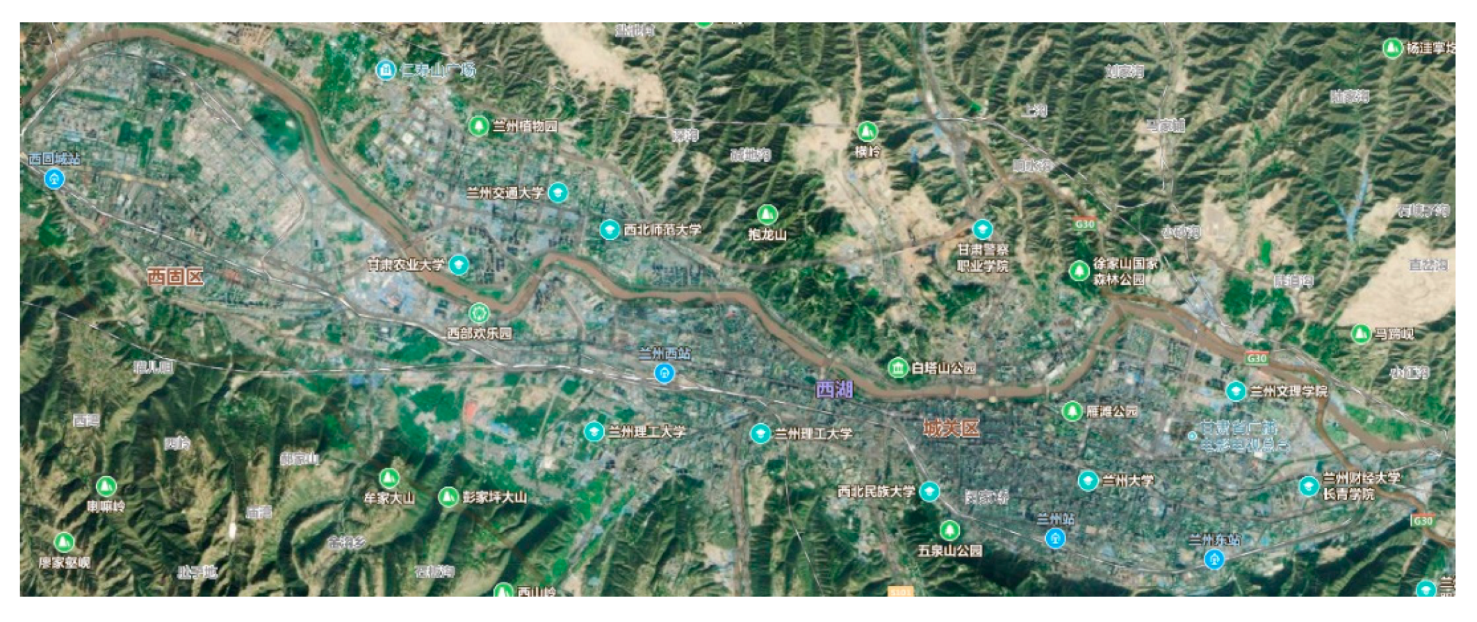
Lanzhou is an important tourist city in China. The city is an important comprehensive transportation hub. At present, the resident population in Lanzhou City is more than 3.6 million, and the number of cars is more than 1.04 million. Urban transportation problems are prominent in the city because of the large population and cars. The spatial layout of Lanzhou is shown in Figure 3.

Nowadays, the construction of electric carsharing stations is based on experience. Thus, optimization of the entire region is difficult. As a result, the company spends a lot of time and resources in operating. Therefore, the rational construction of an electric carsharing location model helps companies reduce blind investment and improve operating efficiency in station optimization. This research applies the location optimization model to optimize the electric carsharing station in Lanzhou.

4.2. Parameter Calibration

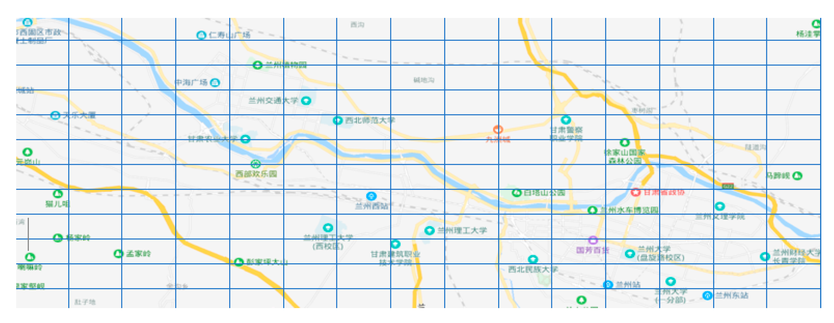
Lanzhou is a strip-shaped city. This research selects a rectangular research area of 30 km × 12 km in Lanzhou and divides the research area into small areas of 2 km × 1 km. A total of 15 × 12 area is obtained. The specific division is shown in Figure 4.

The demand for electric carsharing D is obtained according to the survey done by the carsharing company. Seven types of land use, namely, transportation hubs, ordinary interchange point, business districts, college campuses, jobs, residential areas, and tourist attractions, have significant effects on the demand for electric carsharing. Using Equation (2), the final carsharing demand matrix is obtained.

We divide the area by a grid of 12 rows and 15 columns and set the fixed station placement plan B as a matrix of 12 rows and 15 columns. K is the free station placement plan. In this research, the location of the free station is preset. Therefore, the capacity of the free station needs to be optimized.

$$K=\left[\begin{array}{lllllllllllllll}0& 0& 0& 0& 0& 0& 0& 0& 0& 0& 0& 0& 0& 0& 0\\ 0& 0& 0& 0& 0& 0& 0& 0& 0& 0& 0& 0& 0& 0& 0\\ 0& 0& 0& 0& k_{2,4}& 0& 0& 0& 0& 0& 0& 0& 0& 0& 0\\ k_{3,0}& k_{3,1}& 0& 0& 0& 0& 0& 0& 0& 0& 0& 0& 0& 0& 0\\ k_{4,0}& k_{4,1}& k_{4,2}& 0& 0& 0& 0& 0& 0& 0& 0& 0& 0& 0& 0\\ 0& 0& 0& 0& 0& 0& 0& 0& 0& 0& 0& 0& 0& 0& 0\\ 0& 0& 0& 0& 0& 0& 0& 0& 0& 0& 0& 0& 0& 0& 0\\ 0& 0& 0& 0& 0& 0& 0& k_{7,7}& 0& k_{7,9}& 0& 0& 0& 0& 0\\ 0& 0& 0& 0& 0& 0& 0& 0& k_{8,8}& k_{8,9}& k_{8,10}& 0& k_{8,12}& 0& 0\\ 0& 0& 0& 0& 0& 0& 0& 0& k_{9,8}& k_{9,9}& 0& k_{9,11}& 0& k_{9,13}& k_{9,14}\\ 0& 0& 0& 0& 0& 0& 0& 0& 0& k_{10,9}& k_{10,10}& k_{10,11}& k_{10,12}& 0& 0\\ 0& 0& 0& 0& 0& 0& 0& 0& 0& 0& 0& 0& k_{11,12}& 0& 0\end{array}\right]$$

The service capacity $R_{uv}$ and demand $P_{uv}$ of a single car rental station are generally closely related to the location and capacity of the electric carsharing at the station. It is given by the electric carsharing company based on its own investment level and development strategy. Service intensity usually decreases as the distance to the center of the carsharing station increases. Thus, this research divides the district into core, secondary, and marginal districts. Then, the service matrix of each station can be constructed. This study supposes that a single station has same service capabilities A.

$$A=\left[\begin{array}{l}2\%10\%2\%\\ 10\%45\%10\%\\ 2\%10\%2\%\end{array}\right]$$

V is the average monthly rent matrix per square meter in each small grid.

$$V=\left[\begin{array}{lllllllllllllll}2& 3& 1& 2& 2& 2& 2& 2& 4& 3& 3& 3& 3& 2& 2\\ 2& 2& 3& 7& 5& 5& 5& 2& 8& 3& 4& 5& 7& 4& 2\\ 15& 10& 8& 7& 5& 5& 5& 2& 8& 3& 4& 5& 7& 4& 2\\ 25& 26& 15& 13& 8& 6& 14& 12& 11& 11& 11& 8& 8& 5& 10\\ 24& 24& 18& 12& 12& 10& 10& 10& 10& 7& 14& 12& 11& 10& 8\\ 11& 12& 10& 10& 10& 10& 8& 8& 7& 7& 4& 5& 7& 10& 10\\ 4& 4& 3& 6& 5& 5& 8& 8& 8& 9& 16& 7& 7& 9& 9\\ 4& 4& 3& 6& 5& 9& 10& 10& 10& 30& 20& 20& 15& 15& 15\\ 8& 5& 5& 8& 6& 9& 10& 10& 10& 30& 30& 20& 20& 20& 20\\ 2& 3& 3& 5& 8& 8& 8& 8& 10& 25& 25& 30& 20& 19& 17\\ 3& 2& 2& 3& 4& 4& 6& 8& 8& 15& 20& 24& 20& 15& 15\\ 2& 2& 3& 3& 3& 3& 5& 7& 5& 3& 8& 10& 25& 20& 10\end{array}\right]$$

J is the parking price per hour in the free parking area.

$$J=\left[\begin{array}{lllllllllllllll}0& 0& 0& 0& 0& 0& 0& 0& 0& 0& 0& 0& 0& 0& 0\\ 0& 0& 0& 0& 0& 0& 0& 0& 0& 0& 0& 0& 0& 0& 0\\ 0& 0& 0& 0& 6& 0& 0& 0& 0& 0& 0& 0& 0& 0& 0\\ 8& 8& 0& 0& 0& 0& 0& 0& 0& 0& 0& 0& 0& 0& 0\\ 3& 7& 3& 0& 0& 0& 0& 0& 0& 0& 0& 0& 0& 0& 0\\ 0& 0& 0& 0& 0& 0& 0& 0& 0& 0& 0& 0& 0& 0& 0\\ 0& 0& 0& 0& 0& 0& 0& 0& 0& 0& 0& 0& 0& 0& 0\\ 0& 0& 0& 0& 0& 0& 0& 3& 0& 7& 0& 0& 0& 0& 0\\ 0& 0& 0& 0& 0& 0& 0& 0& 3& 8& 6& 0& 6& 0& 0\\ 0& 0& 0& 0& 0& 0& 0& 0& 3& 3& 0& 5& 0& 6& 6\\ 0& 0& 0& 0& 0& 0& 0& 0& 0& 2& 3& 5& 2& 0& 0\\ 0& 0& 0& 0& 0& 0& 0& 0& 0& 0& 0& 0& 5& 0& 0\end{array}\right]$$

The company intends to invest W = 50 million in these costs.

The cost of buying each car is b = 100,000 yuan.

The construction cost of each charger is e= 2000 yuan.

The average parking time for each car in the free parking area is t = 1440 h a year.

The corresponding coefficient μ = 20 of the area of the stations and the size of the stations.

The corresponding coefficient λ = 0.5 between the scale of the stations and the required number of chargers.

The maximum number of cars dropped at each station is 100.

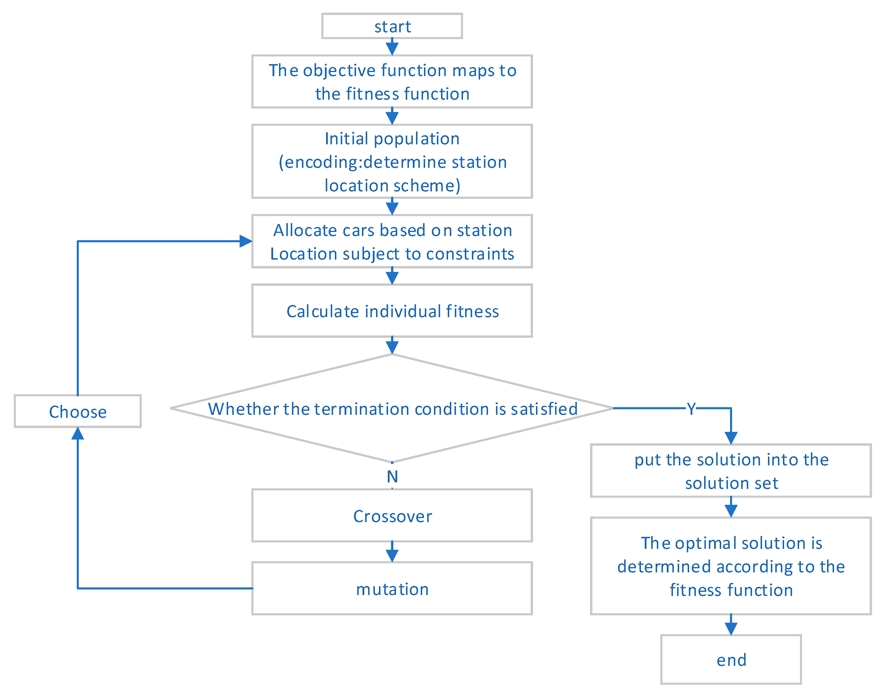
We design a genetic optimization algorithm to solve the model. The calculation process of the algorithm is shown in Figure 2. The corresponding parameters are set as follows:

The selection operator is tournament selection;

The crossover operator is single-point crossover;

The crossover probability is 0.8;

The mutation operator is multipoint mutation;

The mutation probability is 0.05;

The population size is set to 500;

The stop rule is set to a maximum of 600 iterations.

4.3. Results

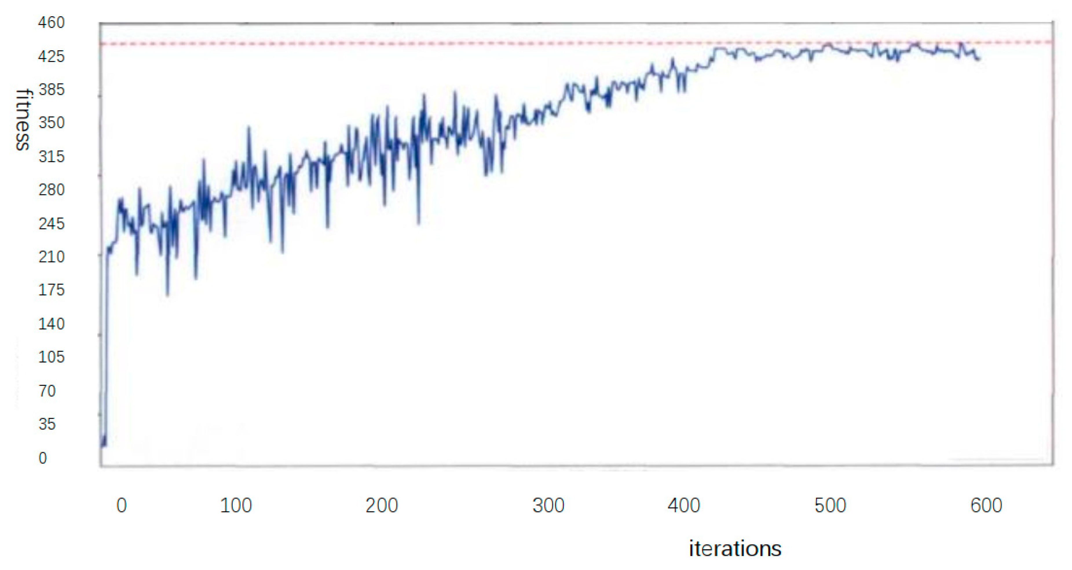
The generated genetic algorithm iterative curve is shown in Figure 5. The figure shows that the genetic algorithm iterative curve shows a rising trend, which is consistent with the optimization model established in this study. Specifically, before the 400th generation the speed of rising is evident, and the degree of dispersion is large. After the 400th generation, the curve is stable, and the fluctuations are reduced. The latter trend continues to the end of the iteration. Therefore, the genetic algorithm converges, and the optimal value of 426 of the stationary period is taken as the optimal solution of the algorithm.

Figure 6 shows the result of superimposing the service range of the electric carsharing network calculated by the genetic algorithm and the demand range of the demand matrix. As observed, the scope of requirements can be surrounded by the service matrix, which indicates that the requirements can be met. Furthermore, the demands are mainly distributed diagonally, which is similar to the demand matrix and the actual situation.

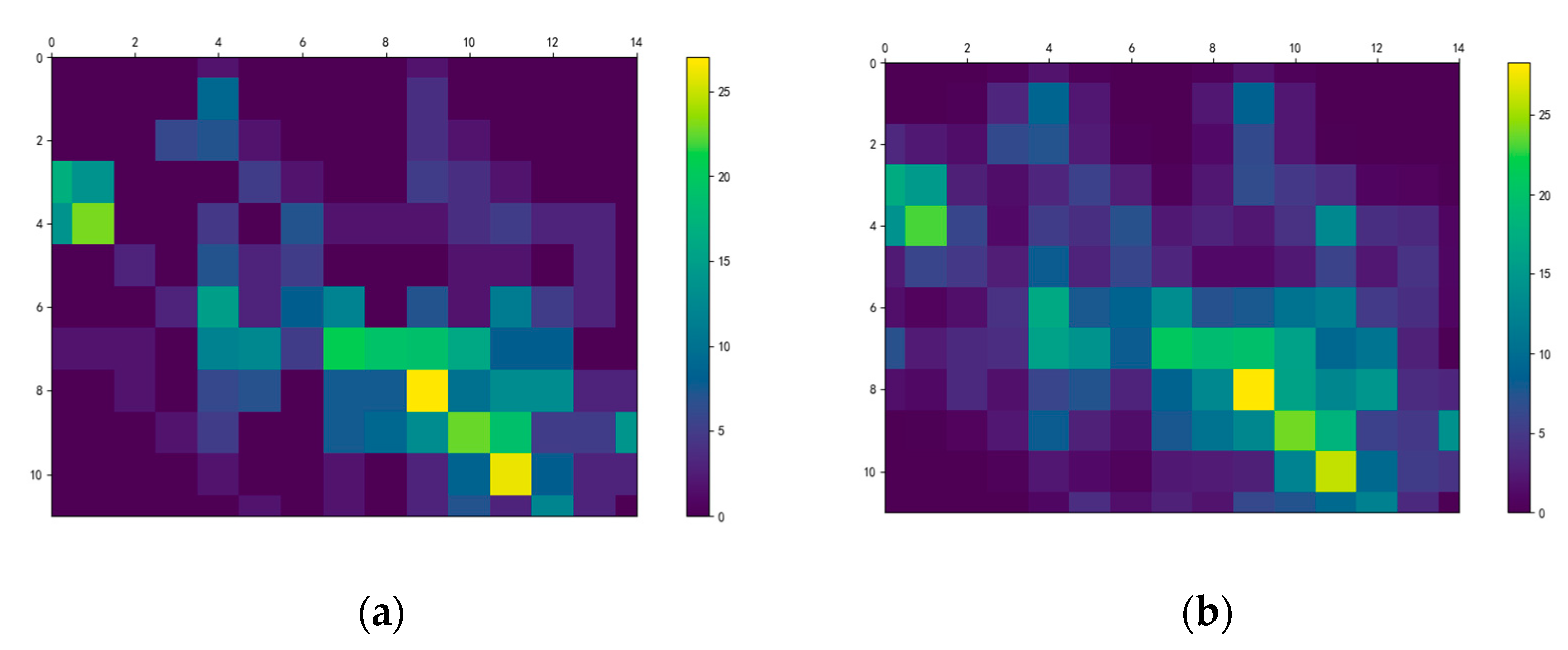
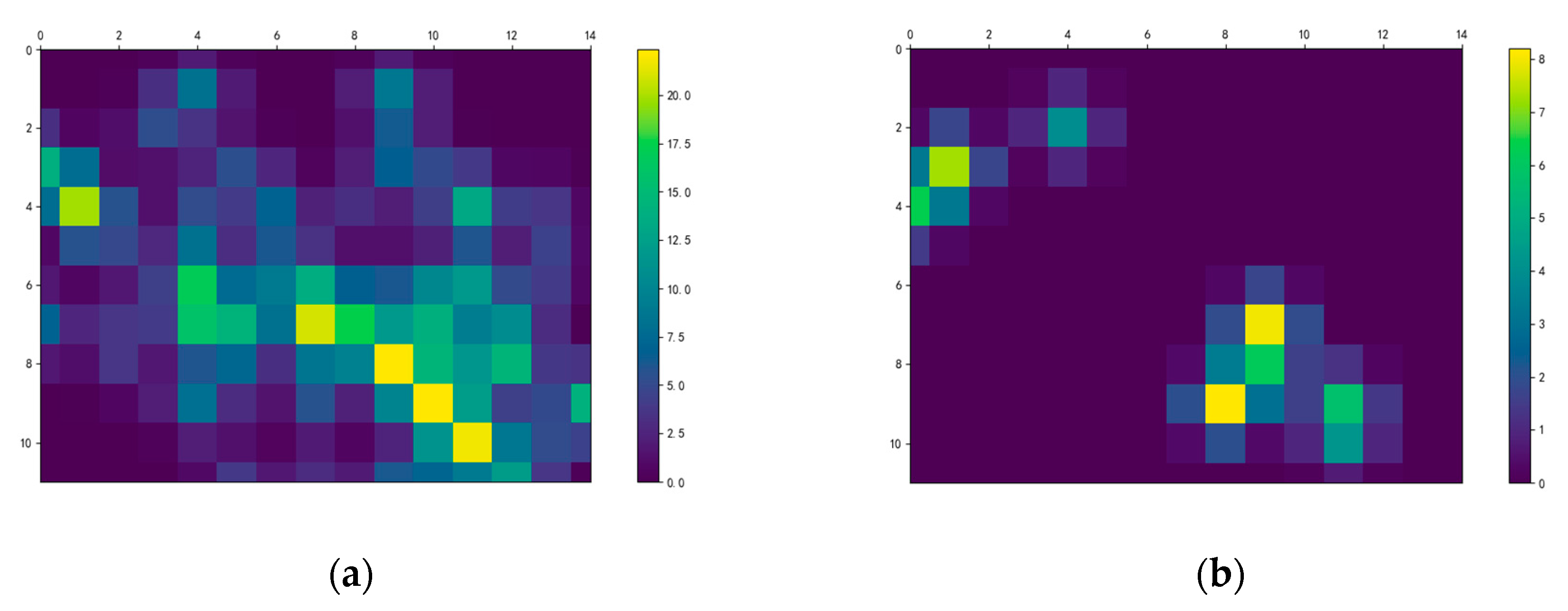
This research meets the overall demands of the city by placing cars in free stations or fixed stations, as shown in Figure 7 and Figure 8. Figure 7 shows the demand range (left) and overall service ability (right) of free and fixed stations. The lighter the color, the larger the quantity, and vice versa. Figure 8 shows the service capabilities and scope of fixed and free sites. The lighter the color, the greater the service capability, and vice versa.

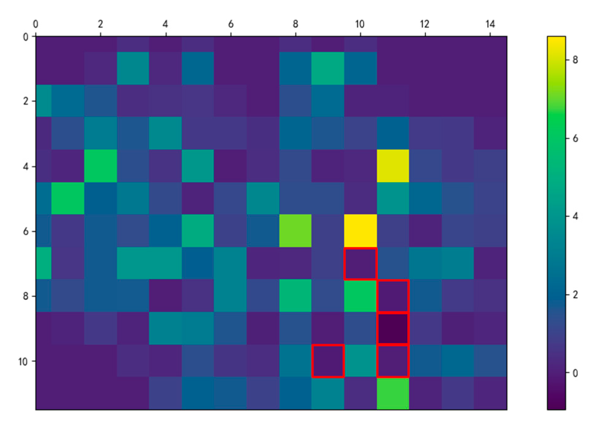
Figure 9 presents the heat map for the final network of the stations. Color shades represent the number of services available minus the number of requirements. The figure shows that user demands can be met in most areas. Some cases in the red grid have demands that are not met.

The specific statistics of the station planning are shown in

Table 1. Statistical table of the arrangement plan.

Station Type	Station Number	Maximum Number of Cars	Car Number Installed
Free station	8	8	44
Fix station	50	20	381
All station	56	24	425

. The entire area must be resettled at 56 regional points, of which two points are required to set stations at free and fixed stations. A maximum of 24 cars can be installed in a single area. A total of 425 vehicles are settled.

5. Conclusions and Prospects

The rapid development of the electric carsharing industry has made the way to locate and design electric carsharing stations a critical issue. This study analyzes the development status and existing problems of electric carsharing. An electric carsharing station location model is established in consideration of multiple influencing factors. The main factors for the demand of electric carsharing are summarized by studying the application scenarios and business models of electric carsharing. On the basis of these factors, a quantitative method that allocates cars according to travel demand is proposed. A model of station location is established on the basis of a two-dimensional spatial analysis. A genetic algorithm is designed to solve the problem given the characteristics of the model. The feasibility of the model and solution method is verified using a case study of Lanzhou.

This research can be used for carsharing station location optimization in a new city. A comprehensive station location optimization model is constructed by considering factors, such as the total number of people in the city, the proportion of travel modes, station construction costs, and construction budget. This method can also be used to study the locations of shared bicycles, electric vehicle charging piles, and logistics distribution points. Therefore, this method can be extended.

The station location problem of electric carsharing is a multi-disciplinary problem and has many influencing factors. On the basis of the analysis and summary of the development status of electric carsharing, this study establishes a network location model and the solution methods. The proposed methods can be improved from the following aspects. First, the forecast of the overall demand for electric carsharing in the region is insufficiently accurate. This study only quantitatively predicts the demand from several macro data indicators. Relatively few influencing factors are considered, and the correlation between the factors has not been studied and verified with examples. Further research is needed. Second, some parameters use an average estimation method that may be inconsistent with actual operations. Finally, the model also ignores the effect of other operators on the regional demand. These issues will be complemented in the future research.

References

1. Sai, Q.; Bi, J.; Xie, D.; Guan, W. Identifying and Predicting the Expenditure Level Characteristics of Car-Sharing Users Based on the Empirical Data. Sustainability 2019, 11, 6689. [Google Scholar] [CrossRef] [Green Version]
2. Chen, W.; Yang, R.; Yang, H. Research on the Status Quo, Problems and Countermeasures of New Energy Vehicle Time-sharing Development in China—Taking the “EVCARD” Model of Shanghai as an Example. Compr. Transp. 2017, 8, 89–92. [Google Scholar]
3. Jorge, D.; Correia, G.H.; Barnhart, C. Comparing Optimal Relocation Operations with Simulated Relocation Policies in One-Way Carsharing Systems. IEEE Trans. Intell. Transp. Syst. 2014, 15, 1667–1675. [Google Scholar] [CrossRef] [Green Version]
4. Du, Z.; Huang, X.; Ding, T.; Li, Z. Discussion on the Development Dilemma of China’s Automobile Time-sharing Leasing. Automob. Pract. Technol. 2017, 19, 1–3. [Google Scholar]
5. Zhang, Z. Some Suggestions on Promoting the Healthy Development of Car Time-sharing Leasing. Transp. Transp. 2017, 33, 27–28. [Google Scholar]
6. Zhao, Z. Problems and Solutions of Time-sharing Rental Service of Electric Vehicles in China. J. Longdong Univ. 2017, 28, 132–134. [Google Scholar]
7. Lu, T.; Huang, J.; Jiang, W. Construction of carsharing network site optimization model: Taking Hongshan District of Wuhan as an example. J. Transp. Res. 2017, 3, 8–15. [Google Scholar]
8. Zhu, R. Finance Leasing Paves Way for New Energy Vehicles in China. Chinas Foreign Trade 2015, 1, 34. [Google Scholar]
9. Chu, F. Explosive growth! The car sharing market is developing rapidly. Transp. Manag. World 2016, 13, 44–45. [Google Scholar]
10. Sawik, B.; Faulin, J.; Perez-Bernabeu, E. Selected Multi-Criteria Green Vehicle Routing Problems; Applications of Management Science Book Series: Applications of Management Science; Emerald: Bingley, UK, 2017; Volume 18, pp. 57–83. [Google Scholar]
11. Ciari, F.; Weis, C.; Balac, M. Evaluating the influence of carsharing stations’ location on potential membership: A Swiss case study. EURO J. Transp. Logist. 2016, 5, 345–369. [Google Scholar] [CrossRef]
12. De Almeida Correia, G.H.; Antunes, A.P. Optimization approach to depot location and trip selection in one-way carsharing systems. Transp. Res. Part E Logist. Transp. Rev. 2012, 48, 233–247. [Google Scholar] [CrossRef]
13. Jiang, B. Research on Vehicle Supply-Demand Matching under Shared Leasing Model; Hefei University of Technology: Hefei, China, 2017. [Google Scholar]
14. Lu, L. Research on Location Optimization of “carsharing” Based on Interval Intuitionistic Fuzzy Soft Set Method Based on Risk Preference. Business 2017, 15, 214–216. [Google Scholar]
15. Çalık, H.; Fortz, B. A Benders decomposition method for locating stations in a one-way electric car sharing system under demand uncertainty. Transp. Res. Part B Methodol. 2019, 125, 121–150. [Google Scholar] [CrossRef] [Green Version]
16. Hu, L.; Liu, Y. Joint design of parking capacities and fleet size for one-way station-based carsharing systems with road congestion constraints. Transp. Res. Part B Methodol. 2016, 93, 268–299. [Google Scholar] [CrossRef]
17. Wielinski, G.; Trepanier, M.; Morency, C. Exploring Service Usage and Activity Space Evolution in a Free-Floating Carsharing Service. Transp. Res. Rec. 2019, 2673, 36–49. [Google Scholar] [CrossRef]
18. Zheng, J.; Qi, G. Location of Charging Stations for Unidirectional Electric carsharing Systems under Fund Constraints. Appl. Comput. Syst. 2019, 28, 208–214. [Google Scholar]
19. Lee, J.B.; Byun, W.; Lee, S.H.; Do, M. Correlation between optimal carsharing locations and carbon dioxide emissions in urban areas. Int. J. Environ. Sci. Technol. 2014, 11, 2319–2328. [Google Scholar] [CrossRef]
20. Chen, Z.; Qin, K.; Liu, K. Genetic Algorithm-Based Location Optimization and Optimization Design of Carsharing Stations. Jiangsu Sci. Technol. Inf. 2019, 36, 39–41. [Google Scholar]
21. Zhu, X.; Li, J.; Liu, Z.; Yang, F. Optimization Approach to Depot Location in Car Sharing Systems with Big Data. In Proceedings of the IEEE International Congress on Big Data, New York, NY, USA, 27 June–2 July 2015. [Google Scholar]
22. Shoufeng, L.; Ximin, L. Based on Hybrid Genetic Algorithm and Cellular Automata Combined Traffic Signal Control and Route Guidance. In Proceedings of the 2007 Chinese Control Conference, Changsha, China, 26–31 July 2007. [Google Scholar]
23. Cheng, Y. Game Study on Urban Transportation Trip Modes under CarSharing; Harbin Institute of Technology: Harbin, China, 2015. [Google Scholar]
24. Deng, Y.; Cardin, M.A. Integrating operational decisions into the planning of one-way vehicle-sharing systems under uncertainty. Transp. Res. Part C Emerg. Technol. 2018, 86, 407–424. [Google Scholar] [CrossRef] [Green Version]
25. Thomas, D.; Kovoor, B.C. A Genetic Algorithm Approach to Autonomous Smart Vehicle Parking system. Procedia Comput. Sci. 2018, 125, 68–76. [Google Scholar] [CrossRef]
26. Wu, Y.; Yang, X.; Zheng, Z. Research on Optimized Layout of Carsharing Parking Places Based on Improved Genetic Algorithm. Logist. Sci. Technol. 2017, 40, 78–82. [Google Scholar]
27. He, L.; Tang, C.; Zhou, R.; Hou, X. Research on SDN enhanced path boxing problem based on genetic algorithm. Comput. Technol. Dev. 2019, 7, 1–4. [Google Scholar]
28. Clarke, D.D.; Forsyth, R.; Wright, R. Behavioural factors in accidents at road junctions: The use of a genetic algorithm to extract descriptive rules from police case files. Accid. Anal. Prev. 1998, 30, 223–234. [Google Scholar] [CrossRef]
29. Ceylan, H.; Bell, M.G.H. Traffic signal timing optimisation based on genetic algorithm approach, including drivers’ routing. Transp. Res. Part B Methodol. 2004, 38, 329–342. [Google Scholar] [CrossRef]
30. Zhang, Q. Design and implementation of optimization algorithm for traffic line selection based on genetic algorithm. Comput. Eng. Appl. 2009, 45, 226–228. [Google Scholar]
Figure 1. Schematic of the study area meshing.
Algorithms 13 00043 g001
Figure 2. Flowchart of genetic algorithm processing.
Algorithms 13 00043 g002
Figure 3. Spatial layout of the study area.
Algorithms 13 00043 g003
Figure 4. Diagram of area division.
Algorithms 13 00043 g004
Figure 5. Graph of the iterative process of genetic algorithm.
Algorithms 13 00043 g005
Figure 6. Bubble chart of service and demand ranges.
Algorithms 13 00043 g006
Figure 7. (a) Thermal map of demand range and (b) overall service range.
Algorithms 13 00043 g007
Figure 8. (a) Thermal map of the fixed station and (b) free station service range.
Algorithms 13 00043 g008
Figure 9. Thermal map of the service excess matrix.
Algorithms 13 00043 g009