Abstract
To manage multidimensional point data more efficiently, this paper presents an improvement, called HD-tree, of a previous indexing method, called D-tree. Both structures combine quadtree-like partitioning (using integer shift operations without storing internal nodes, but only leaves) and hash tables (for searching for the nodes stored). However, the HD-tree follows a brand-new decomposition strategy, which is called half decomposition strategy. This improvement avoids the generation of nodes containing only a small amount of data and the sequential search of the hash table, so that it can save storage space while having faster I/O and better time performance when building the tree and querying data. The results demonstrate convincingly that the time and space performance of HD-tree is better than that of D-tree regardless of uniform or uneven data, which are less affected by data distribution.
1. Introduction
In recent years, with the rapid development of positioning and mobile technology [1], a mass of applications have produced a large amount of data with different characteristics, such as spatial characteristics and temporal characteristics. Spatial characteristics are usually represented by spatial objects, such as point, line, polygon, etc. These spatial objects can be organized by one or more coordinates. In large-scale spatial analysis applications, the management of massive coordinates is an essential basic work. The management of coordinates can be regarded as the management of points. Therefore, this paper studies the management of large-scale point data.
If you want to improve the efficiency of data retrieval, an appropriate index is essential. However, the indexing of high-dimensional data can be difficult because as the number of dimensions increases, the time and space costs of indexing increase dramatically. For large dimensions (20 is already enough), the indexing performance will be degraded to the most primitive sequential search, which is called ’curse of dimensionality’ [2]. Nowadays, with the rapid development of big data [3] and cloud computing [4], generating massive complex high-dimensional spatial data needs a continuously updated index, as well as a quicker response, so a dynamic index is urgently needed.
In the past decades, people have put forward a large number of index structures and methods to support the retrieval of data, and some of them have been widely used. Compared with other types of indexing, the easiest and most straightforward method to retrieve the data is the linear indexing which filters out the required data one by one from a data set. There is no doubt that the results can be accurately found in this way. However, the efficiency is obviously unacceptable. Another classical method is the hash table [5]. Theoretically, the time complexity it takes to find a piece of data is O(1) which is remarkable. However, the classic hash table is mainly engaged in exact matching search and it is extremely difficult to implement range queries.
Another type of indexing adopts a tree structure. It performs well for its limit time complexity is usually O(lgn). In addition, it can execute range queries. The majority of spatial data indexes adopt a tree structure, such as R-tree, KD-tree, B-tree and X-tree [6]. They can be classified according to two ways, one is the way of data partition, the other is the way of space partition.
Space partition trees are partitioned typically by space filling curve or the classification of each dimension of the space. The advantages of the space filling curve are that the data of any dimensions can be processed, and the data can be mapped to the one-dimensional space for coding, so that the existing B-tree [7], B-tree [8], hash table and others can be used to perform one-dimensional space query. However, the obvious disadvantage is that at least one of them should be recoded when the indexes of different regions are combined. The index using space filling curve is extremely difficult to code in high dimensions, which makes implementation quite hard. In addition, when this method is used for range queries, there is usually a defect that some data mapping deviation is too large.
There are some trees divided according to the classification of each dimension in the space, such as KD-tree [9], B-tree, etc. Firstly, they have many sub-trees in high-dimensional space. Secondly, the imbalance of the tree structure causes deeper depth of the tree, which will degrade performance and cause problems to search in a high-dimensional space. What is more, the query operation and insertion operation of these trees may be simple, while the delete operation may be more complicated because of its rebuilt sub-trees caused by the deletion of a node. There are also some variants based on KD-tree or B-tree, such as KDB-tree [10], B tree [11], B-tree [8], B-tree [12]. Although they can maintain the balance of a tree, it will consume a lot of time and space, and thus reduce the efficiency of frequent data manipulation.
The spatial indexes divided by data are mainly presented as R-tree [13] and its variants, including R-tree [14], R-tree [15], TPR-tree [16], RTR-tree [17], etc. These trees represent spatial objects by using the minimum bounding rectangle. The data overhead might be greater than the spatial objects themselves. Although many improved trees have solved the overlapping to some extent, the overlapping in high-dimensional space is still very serious, and thus lower the indexing efficiency.
Several other methods can combine grid indexes with other indexes, for example, the combination of quadtrees [18] and hash tables. One of the most advanced methods is the decomposition tree (D-tree) [19]. D-tree adopts the principle of spatial partition and integer encoding shift operations to determine the range of multidimensional space. It does not need to store the spatial range of the node and the keywords of the child nodes, and thus no additional disk access is required when looking for leaf nodes. As a result that D-tree itself is a discrete linear structure without inner nodes, it is easy to implement parallel access and can perform excellently.
However, since D-tree adopts the full decomposition strategy to allocate all spatial objects to child nodes on the principle of spatial partition, more child nodes are decomposed, which makes range queries require more disk access. In addition, when the spatial node and its upper node do not exist, a large number of lookups to the hash table are required and it will reduce efficiency sharply. In view of these shortcomings, in this paper, we proposed a high-dimensional spatial index based on D-tree—the half decomposition tree (HD-Tree).
HD-tree’s decomposition will generate a new node containing more spatial objects from an original node, which allows it to retain the original and new nodes based on the structure of the virtual tree. Therefore it can reduce space consumption and improve time efficiency. The experimental comparison results show that under normal circumstances, the space, time and I/O times of the HD-tree are less than those of D-tree, especially when the data are unevenly distributed.
The rest of this paper is organized as follows: in the next section, we will review the decomposition strategy and indexing structure of D-tree. In Section 3, we describe the half decomposition strategy, structure and algorithms of HD-tree. In Section 4, we describe the experimental results and analysis. Finally, in Section 5, we will summarize.
2. Background
2.1. Concepts
Some concepts are important for this paper. In this subsection, we illustrate the main features of concepts.
- I/OI/Os include network I/O and disk I/O. The I/O mentioned in this article refers to disk I/O.To reduce the number of disk I/Os is the main goal of index optimization.
- RectangleThe rectangle [19] in this article represents a range of space, not just 2 dimensions, but possibly many, with a minimum and a maximum on each dimension. For example, a 4-dimensional rectangle has an X-axis range of [0,10], Y-axis range of [10,30], z-axis range of [20,30] and v-axis range of [10–20].
- Basic rectangleThe basic [19] rectangle is a rectangle described above. It is the rectangle range corresponding to the root node, and the rectangle range corresponding to other nodes is contained by the base rectangle.
- Prefix encodingOne prefix encoding [20] can be obtained by right-shifting another encoding. For example, in a 4-dimensional space, using hexadecimal encoding, an integer encoding 0 × 165 can give 0 × 16 and 0 × 1 after right shifting, so 0 × 16 and 0 × 1 are prefix codes of 0 × 165. Similarly, 0 × 165 is the suffix encoding for 0 × 1 and 0 × 16.
- Point objectA point object is a collection of values in various dimensions of a point in space. For example, a collection of 4-dimensional points may be [20,10,23,40]. A point object may also be a collection of strings or other types, as long as it can be distinguished from other point objects according to its characteristics.
- Point queryQuerying the node to which a point object belongs in the tree is called a point query [21]. Point query needs to find the node it belongs to, and then compare it with the spatial object contained by the node in turn.
- Range queryThe range query [21] can also be called a rectangular query. This article deals with point objects, so a range query needs to find all the point objects contained in the rectangle from the tree.
2.2. D-Tree
The half decomposition tree (HD-tree) described in this paper is proposed to improve shortcomings of D-tree. In order to clearly understand the improvement mechanism of HD-tree, it is necessary to comprehend the design principles of D-tree, including the full decomposition strategy, coding method, index structure, etc.
The D-tree is a virtual tree whose core idea is to determine the spatial position through the spatial dichotomy method combined with integer shift operations. Its decomposition strategy will decompose the space into subspaces of the same size according to the principle of space division when the spatial objects contained in a space exceed the maximum limit. After encoding these subspaces, those spatial objects will be transferred to the nodes corresponding to subspaces. For example, if the dimension of a space is 2, the space can be decomposed into four subspaces with the binary codes of 100, 101, 110, 111. The binary code for the basic rectangle cannot be 0, and if it is 0, its subrectangle code can also be 0, so you cannot distinguish between them. In this way, each space has a unique integer encoding, and the node corresponding to the encoding can be applied to store spatial objects. The hierarchical relationships of D-tree are implicated by the integer code of each leaf node, so we can easily calculate the range via an integer code and compute a code, which corresponds to a range.
As shown in Figure 1, this is an example of partitioning and encoding of a three-dimensional space. Assume that the integer code of the basic rectangle is 1, the space can be divided into eight subspaces of the same size after dichotomy along the three dimensions of x, y and z, and then the corresponding octal codes are from 010 to 017. Similarly, subspaces can continue to be decomposed. For example, the space represented by 010 can be decomposed into eight subspaces encoded starting from 0100.
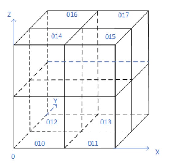
Figure 1.
Space partition and coding.
The D-tree is essentially a gird-based index structure. The unbalanced grid index may result in a large depth of the tree, which usually demands more I/O consumption when indexing, while the D-tree can reduce I/O times by integer shift operations without accessing those inner nodes and leaf nodes without data. Furthermore, it can save the storage space by omitting those nodes mentioned above.
Figure 2 shows an example of a four-dimensional D-tree in the paper of D-tree. As a result of the virtual tree, the non-leaf nodes 0 × 1, 0 × 10, 0 × 18, 0 × 18b and 0 × 18c are not stored, and those nodes without data are not displayed in the figure and need not be stored. The number of nodes of a full balanced hex tree whose depth is four is equal to 4396. In the example of D-tree, it only needs to store 9 leaf nodes with data after space division and encoding. The commonly used balanced tree structure requires n (n is the depth of the tree) disk visits to access a leaf node, but with D-tree, we can access the leaf node by computing integer encoding, with no need to go through the middle node, as we only need one disk visit (assuming the hash table is in memory, disk access to the hash table is not required).
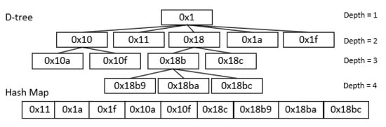
Figure 2.
Example of four-dimensional decomposition tree (D-tree).
Although the performance of the D-tree is excellent, it still has some deficiencies. The full decomposition strategy of the D-tree results in more leaf nodes, and the number of I/Os is larger when executing a range query. Suppose, in a four-dimensional space, when the number of spatial objects of a node reaches the limit, 16 leaf nodes may be required after a D-tree’s decomposition, because 16 subspaces may all contain objects. If a node is mapped to a disk page, the D-tree may require at least 16 I/Os to query the range represented by the original node, which is is hard to accept. Moreover, the D-tree may need enormous lookups to the hash table when performing insertion operation, which will seriously affect efficiency. The hash table in the D-tree is used to determine whether the integer encoding of a certain position exists. Theoretically, the query time complexity can reach O(1). However, when the code and its upper codes do not exist in the hash table, a large number of lookups will need to be performed on the hash table until the same level code or the same level code of prefix code can be found. This means that D-tree needs to determine the level of the leaf node, and establish a node in the same layer to insert data. The query time complexity will seriously degrade to O(n) at this time. There are two ways to look up an encoding in a hash table to see if it has a suffix encoding. One is to look up each suffix code of the integer code to determine if a suffix code exists in the hash table, and the other is to traverse all the values in the hash table until there is a value that is the suffix code of the integer encoding. Generally speaking, the first method is more efficient when the distribution of data is relatively balanced, and the second method is more efficient when the data are relatively uneven. The specific use of this method depends on the actual situation. In the parer of D-tree, the second method is used by default.
In consideration of the shortcomings of D-tree, we propose a novel high-dimensional spatial index than we have named the half decomposition tree (HD-tree). It can reduce space consumption, time cost and I/O times. In the next section, we will introduce fundamentals and algorithm implementations of HD-tree.
3. Methodology
3.1. Half Decomposition Strategy and Index Structure of HD-Tree
By studying the B-tree optimization of the B-tree, we find that the B-tree stores all the data in the leaf nodes, and the inner nodes only store the indexed keywords without storing the data. This allows the inner nodes to hold more keywords. The more keywords that are read into memory at one time while indexing, the fewer the relative I/O times. This also gives us an inspiration. The B-tree needs to maintain the tree structure, while the D-tree adopts a virtual tree structure which does not require the use of inner nodes to store index keywords. Why not use it to store data? Therefore, in this paper, an improvement based on the D-tree is proposed, which we call the half decomposition tree (HD-tree). The dichotomy of each dimension of the space used by the HD-tree is the same as that of the D-tree, but different decomposition strategies are adopted. The full decomposition strategy of the D-tree divides the spatial objects in the multidimensional space into the subspaces to which they belong. The half decomposition strategy of the HD-tree will select the subspace containing more spatial objects in the space, generate a new spatial node and keep the remaining spatial objects in the original spatial node. It can reduce space consumption and increase time efficiency by the half decomposition strategy.
As shown in Figure 3, the Figure 3a is a D-tree and the Figure 3b is an HD-tree. We use a hash table to store the encoding of these nodes, which can help us determine whether the encoding of a node exists in the tree with the time complexity of O(1). However, the space complexity of hash table is relatively high, and a large number of elements will have a great impact on the storage space. Therefore, if not necessary, we should minimize the number of elements in the hash table. Assume that a node can store up to 32 spatial objects. The number of spatial objects stored in a node is represented by the number in parentheses in the figure. When the number of spatial objects in a space exceeds the limit and the data are distributed in many subspaces, the D-tree will generate more subspace nodes. The 56 spatial objects are managed by D-tree and HD-tree respectively. Using the D-tree, 56 spatial objects still need 12 spatial nodes after removing nodes that do not contain spatial objects. The HD-tree separates the subspace containing more spatial objects until the number of the spatial objects in each spatial node does not exceed the limit. Using the HD-tree, the total 56 spatial objects only need 3 spatial nodes, and each node does not exceed the limit of the number of spatial objects. It can be seen that the half decomposition strategy used by the HD-tree can save some nodes and save the use of the hash table compared to the full decomposition strategy used by the D-tree. When using disk storage, it can reduce the disk space occupied by spatial nodes.
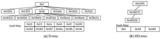
Figure 3.
Example of D-tree and half decomposition tree (HD-tree) in four-dimensional space.
If we access data through a disk, because the number of subspace nodes generated by the HD-tree decomposition process is smaller than the D-tree, the HD-tree has fewer I/Os in the range query. Assuming that each node corresponds to a disk page, reading data within a disk page is equivalent to one I/O. As shown in Figure 3, now we need to get the spatial objects in the range represented by the code 0 × 18. In the D-tree, the node represented by code 0 × 18 does not store data, but its 7 child nodes have data. Then the D-tree needs at least 7 disk I/Os to read the data in its child nodes. The HD-tree needs to access the data in the node represented by 0 × 18 and the child node represented by 0 × 182, which means it only needs two I/Os. The disk I/O is a very expensive operation, and its operating efficiency is very low compared to memory. It is an important reason to limit the throughput of metadata reading and is one of the bottlenecks of distributed clusters. Reducing disk I/Os is quite necessary. This is also an important reason for proposing D-tree and HD-tree.
When performing data insertion, the D-tree first calculates the integer encoding of the space range that can contain the target in the deepest part of the tree. Then move the code forward to determine if it or the prefix codes have one in the hash table. When an integer code exists in the hash table, the insertion operation can be performed on the node represented by the code. Since the D-tree only stores leaf nodes, if a node can be found, it must have no child nodes. However, if each of these integer codes does not exist in the hash table, the D-tree needs to traverse the hash table (Scheme used by D-tree). From the code of the basic range of the tree to the target code, look down in turn. When we find an encoding that has no suffix encoding in the hash table, we can create a new node here to insert the data. This may require traversing the hash table multiple times.
In Figure 3a, suppose we want to insert a spatial object into the D-tree, and its integer encoding at the deepest point of the tree is 0 × 132. Obviously, the three codes 0 × 132, 0 × 13 and 0 × 1 do not exist in the hash table, so it is necessary to start traversing the hash table. We can find the integer encoding prefixed with 0 × 1 in the hash table, such as 0 × 10, but we can’t find a code prefixed with 0 × 13 in the hash table. Then we create a leaf node encoded in 0 × 13 and insert the spatial object into the node. Here, we need to iterate through the hash table twice, and the second time we need to completely traverse the hash table. When the depth of a D-tree is relatively large, and the hash table is large, it may be necessary to traverse the hash table many times, and each traversal may take a long time, which will seriously affect the efficiency of the operation of the data. However, the HD-tree can solve the problem fundamentally. It can guarantee that the deepest integer encoding of the tree corresponding to the target or its upper layer codes must have one in the hash table. The integer encoding of the lower node is generated by the integer shift operation of the upper node. If the node corresponding to the upper integer encoding has no data, the node will be deleted, but the encoding will still be stored in the hash table. Similarly we want to insert a spatial object, and its integer encoding at the deepest point of the tree is 0 × 132. The integer encoding is shifted upward. It can be seen that the codes 0 × 132, 0 × 13 do not exist in the hash table, but the code 0 × 1 exists in the hash table. We only need to insert data into the spatial node represented by 0 × 1, and determine whether the number of spatial objects in the spatial node exceeds the maximum number limit. If the number of spatial objects exceeds, a half decomposition strategy is used for the spatial node. Therefore, the HD-tree can greatly improve the efficiency of the data insertion by improving the decomposition strategy of the D-tree.
In summary, the HD-tree and D-tree adopt different decomposition strategies while maintaining the virtual tree structure. The strategy used by the HD-tree not only enables it to save nodes and thus saves storage space, but also reduces the number of I/Os for range queries. At the same time, the algorithm efficiency of data insertion is improved. In the next subsection, we will introduce some algorithms for HD-tree.
3.2. Algorithms of HD-Tree
The HD-tree is an improvement on the D-tree, so some algorithms similar to the D-tree are not described here or simply described. Suppose the number of dimensions of the basic rectangle is dimension, the basic rectangle is barec, the maximum number of spatial objects that each node can contain is maxsize, the hash table containing codes is hash and the maximum depth of the tree is maxdep.
Our HD-tree consists of a series of nodes. As shown in Figure 4a, a node contains two fields, where the code is the integer encoding of the node, and data are the set of spatial objects contained in the node. The objects in data have a value in each dimension. We use position to represent the set corresponding to these values, namely {a, a … a}. Each node has a corresponding spatial range, and each range query also requires a range. Here we use a rectangle to represent a range. Figure 4b shows the structure of a rectangle. The rectangle has a minimum and a maximum in each dimension.
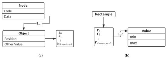
Figure 4.
(a) Structure of spatial node, (b) structure of rectangle.
After introducing some basic data structures, we need to introduce some related functions. The first is V(N,R). Given a node N and a rectangle R, find a set of objects, which are spatial objects in N, and they are included in the range of R, defined as Equation (1).
Given a rectangle R and another rectangle AR. When they meet the conditions in Equation (2), the minimum value of R in each dimension is not greater than the maximum value of AR in the corresponding dimension, and the maximum value of R in each dimension is not less than the maximum value of AR in the corresponding dimension. If the condition is met, indicating that the two rectangles intersect, we return true, otherwise return false. We use G(R, AR) to indicate this judgment condition.
Given a node N and another node LN, we need to find a set of objects, so that these objects are both objects in N, and these objects are included in the range represented by the code corresponding to the node. We write this function as M(N,LN), defined as Equation (3).
Now we begin to formally introduce algorithms. The first algorithm to be introduced is to find the corresponding rectangle in the tree according to the integer code. As shown in Algorithm 1, all values after the highest bit of an encoding are added to the stack in order from low to high (steps 4–5). If a code of a four-dimensional HD-tree is 0 × 123, then 3, 2 are sequentially placed on the stack. The value here represents which sub-rectangle we need after a rectangle decomposition. We pop the values in the stack in order, decompose the rectangle and get the corresponding sub-rectangle until the stack is empty, returning the last sub-rectangle (steps 6–17). How to get the range of the sub-rectangle is shown from step 7 to step 10.
| Algorithm 1:Calculate Rectangle |
 |
When D-tree calculates the integer code of a rectangle or a point at the maximum depth of the tree, a top-down decomposition algorithm is used to obtain an integer code, so that the range represented by the integer code can include the target. In this way, it is necessary to judge the spatial relationship with many unrelated spatial nodes. When the depth of the tree is large, it will be affected to some extent. This paper proposes a bottom-up algorithm to calculate the integer encoding, as shown in Algorithm 2. It finds the integer code based on the relative position of the target range center in the multidimensional space. We know that the space division of the HD-tree adopts the spatial dichotomy principle. Then, as long as the position of the target in the spatial division is determined to be in the first half or the second half, it can be determined whether the integer coding is in the first half or the second half. By analogy, by successively judging each dimension until no space is divided, the sum of all the judgment results is the integer code of the most central point of the target at the deepest point of the tree. Steps 2 and 4 show how to calculate the center of the target range. Calculating the integer code corresponding to the rectangle whose center is in the deepest part of the tree is shown from steps 5 to 11. With this encoding, we can use an integer shift operation like the D-tree until a spatial range represented by an integer encoding can contain the target (steps 12–13).
| Algorithm 2:Calculate Code |
 |
3.2.1. Insertion Algorithm and Deletion Algorithm
The insertion algorithm of the HD-tree is similar to the D-tree. First, the integer encoding of the target at the deepest point of the tree is calculated. Then, find the code or its prefix encodings from bottom to top in the hash table. If one of them can be found in the hash table, it means there is a node, and its corresponding rectangular range can contain the target object we want to insert. That is, we need to insert the target object into this node represented by the code we found. HD-tree can guarantee that the deepest integer encoding of the tree corresponding to the target or its upper layer encoding must have one in the hash table and there is no need to traverse the hash table. When we determine the encoding corresponding to the place to be inserted, we can insert data into the node represented by the encoding. If the number of objects in the node exceeds the maximum value, it is decomposed. Below we will introduce the decomposition algorithm of the HD-tree. Algorithm 3 shows the decomposition process of the HD-tree. The HD-tree adopts the half decomposition strategy. After spatial division, a subspace containing the most spatial objects is selected to generate a new node (steps 4–6). These spatial objects belonging to the new spatial node are added to the new node from the original node (steps 9–10). Then, calculate the depth of the new node, compare it with the original depth and choose a larger value to assign to the depth (step 11). Finally, the original node and the child node are respectively judged whether the spatial object exceeds the maximum limit, and if it exceeds, the decomposition continues, otherwise it ends (steps 12–15).
The deletion of the HD-tree is also similar to the D-tree. Calculate the integer encoding of the target to be deleted in the tree, and then delete the target to be deleted from the node represented by the integer encoding or its child nodes. Finally, it is judged whether the node after deleting the data is empty. If there are no spatial objects in the node and there are no child nodes, then the node can be deleted.
| Algorithm 3:Split Node |
 |
3.2.2. Query Algorithm and Update Algorithm
Point query can be seen as a special case of the range query, so here we only introduce the algorithm of range query. The range query of the HD-tree is shown in Algorithm 4. First, calculate the integer code in the deepest part of the tree for the rectangle to query. If the code is 0, it means the basic rectangle cannot include the target range. The query algorithm needs to be used after the target range and the basic rectangle are intersected (steps 2–3). If the code exists in the hash table, traverse the spatial objects in the node represented by the integer code, and add the spatial objects belonging to the target range to the result (steps 4–9). Then, determine in turn whether the scope represented by the subspace node and the query scope intersect. If the two have intersecting parts, add them to the queue for subsequent processing (steps 10–12). If the calculated code is not 0 and does not belong to the hash table, look up the upper node of the node corresponding to the code in turn (steps 14–19).
Due to the virtual tree structure of the HD-tree, its update is very simple, as long as the target node is found for the relevant data update operation.
| Algorithm 4:Range Query |
 |
4. Experimental Evaluation
In this paper, the dimensions of experimental data are 4, which are the dimensions of spatial-temporal data. We used three different sets of data to compare HD-tree with D-tree from two aspects: data insertion and query. In terms of data insertion, we mainly examine algorithm efficiency and space consumption. The queries contain point matching queries as well as range queries. For point matching queries, we only compare the expenditure of time. For range queries, we compare the algorithm time and I/O times.
The computer configuration is Intel(R) Core(TM) 2.4 GHz 8 Core, 32GB RAM. We use three simulated four-dimensional data sets for experiments. The spatial range of the three sets of data is from [0, 0, 0, 0] to [10,000, 10,000, 10,000, 10,000], and each set of data contains 100 million spatial objects. Since it is difficult to visually show the four dimensional data, we represent the distribution of the three sets of data in the form of two-dimensional projections, corresponding to the three sub-figures in Figure 5. The distribution of the first set of data is Uniform, as shown in Figure 5a. In Figure 5b, the distribution of the second set of data is a Gaussian distribution from the origin; that is, it spreads outward from the origin, and the more outside, the less data. The distribution of the third group of data is shown in Figure 5c. We randomly select 100 positions in the space as the center of each cluster, and distribute 1 million data near each center. Similarly, the further away from the center of the cluster, the less data. The three sub-figures in the subsequent experimental results correspond to the three sets of data mentioned above. Why not choose some existing benchmark data sets? Since the D-tree is a form of spatial division and adopts a full decomposition strategy, it can be guessed that the D-tree is greatly affected by the data distribution. In addition, through experiments, it can also be proved that the data distribution has a great influence on the D-tree. Therefore, we generated three data sets with different distributions which have more obvious characteristics than some existing benchmark data sets and can better reflect the impact of differently distributed data on D-tree and HD-tree.
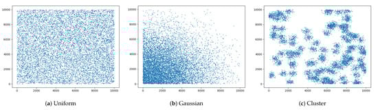
Figure 5.
Projections of three differently distributed data in two dimensions.
4.1. Insertion Performance Evaluation
To evaluate the space usage of HD-tree and D-tree, we set the maximum number of spatial objects allowed in a node to be 128. We continuously insert 100 million spatial objects, reflecting the space utilization of the two trees by the number of nodes, because we use a node to map a disk page. Figure 6a reflects the number of nodes used to insert 100 million spatial objects. When the data distribution is evenly distributed, as the data are continuously inserted, a large number of nodes are quickly decomposed due to the complete decomposition strategy. Then, in the process of inserting data for a long time, there is no decomposition or only a few nodes are decomposed, because the data are evenly distributed, the previously decomposed nodes can also accommodate a large amount of data. Nodes of HD-tree are continuously decomposed with the inserted data; thus, the HD-tree does not occupy many nodes like the D-tree when the data volume is small. It can be seen that no matter what kind of data distribution, the consumption of space of the HD-tree is not higher than the D-tree, especially when the data are unevenly distributed, nearly half of the space can be saved. Although the distribution of the data had an impact on the number of nodes, the HD-tree had a slight impact.
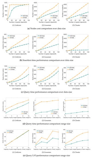
Figure 6.
Experimental comparison.
Figure 6b shows the time taken to insert objects. Regardless of the data distribution, under the same data, the time consumption of the HD-tree is much less than that of the D-tree. In the first two types of data (Uniform and Gaussian), the HD-tree uses only half the time of the D-tree, and the last data (Cluster) consume less than 20% of the time of the D-tree. The main reason is that in the case of uneven data distribution, the probability that the D-tree cannot find the deepest integer code or the upper layer codes is greatly increased. It needs a lot of sequential lookups to the hash table, so the time is greatly increased. In addition, the performance of the insertion of the three data sets of the HD-tree is closer, which means it is less affected by the data distribution.
4.2. Query Performance Evaluation
In this paper, we will compare the query performance of HD-tree and D-tree by point query and range query, respectively. Since disk performance is greatly affected by other factors, we do not compare disk time, but rather the performance of algorithm and the number of I/Os.
Figure 6c reflects the time spent on point queries (100 million spatial objects). The two trees are both virtual tree structures, a single point query only needs one disk I/O, so the I/O of the point query of them is the same, without any significance of comparison. The algorithm performance gap between them can be mainly reflected in three places (i.e., calculate the integer code of the data in the deepest part of the tree, look up the code or its upper codes in turn in the hash table, and traverse the data in the node). According to the experimental results, the algorithm performances of both trees are affected by the data distribution. However, the performance of point queries of the HD-tree is better than the D-tree in the same data.
We measure the efficiency of range queries in terms of algorithm time and I/O quantity. As a result that the location is randomly selected and the data distribution is irregular, when a range query is performed, more time and I/Os may be spent on a smaller range. The entire range of the tested four dimensional data is defined as BV, and the range to be queried is defined as QV. Figure 6d shows the relationship between query time overhead and the size of query range. The horizontal axis represents the ratio of the range QV to be queried to the total range BV. The QV/BV ratio is from 2% to 10% in 2% step. In the experimental results, the time of the range query of the two trees increases linearly. It can be seen from the slope that both are affected by the data distribution. Under evenly distributed data (Uniform), the performance difference between the two is small. The performance of algorithm of HD-tree is significantly better than D-tree when the data are unevenly distributed (Gaussian and Cluster). The reason for this is that when the data are balanced, the number of nodes that the two trees need to find in the range query is the same (In Figure 6e, the experimental results of the data distribution as Uniform can prove this point), and the difference is mainly reflected in the speed of finding the nodes. When it is not balanced, the number of nodes to find also affects the two trees, so the gap is larger than when it is balanced.
In high-dimensional space, the performance of a range query is mainly evaluated by the number of I/Os. Here, we reflect the I/O times by the number of visits to the nodes during the query. Figure 6e shows the change in the number of I/Os as a function of the QV/BV ratio. When the data are evenly distributed (Uniform), the I/O times of the HD-tree are basically equal to those of the D-tree, but the number of I/Os spent is much lower than that of the D-tree when the data are unevenly distributed (Gaussian and Cluster). Under three different data types, the number of I/Os of HD-tree is closer, which is less affected by data, but the number of I/Os in D-tree is greatly increased when the data distribution is uneven. Compared with Figure 6a, it can be found that the number of I/Os is affected by the number of nodes during range query.
By summarizing the analysis of the above insert operations and query operations, we can know that HD-tree is not lower than D-tree in terms of space usage, insert performance, range query performance, etc. Generally speaking, the performance of the HD-tree is better than the D-tree, especially when the data are unevenly distributed, its performance is far better than the D-tree. In addition, the performance of HD-tree is less affected by the data than D-tree.
5. Conclusions
In this paper, we firstly introduced some high-dimensional indexing solutions that have been widely used and their deficiencies. Then we introduced one of the most efficient methods, D-tree, and analyzed its problems. On this basis, a high-dimensional spatial index structure, the half decomposition tree (HD-tree) is presented. The HD-tree adopts different decomposition strategies under the premise of the virtual tree structure of D-tree. Compared to D-tree, it has been greatly optimized through the half decomposition strategy (i.e., reducing the number of spatial nodes, which optimizes the space utilization; avoiding a large number of lookups to the hash table, which will greatly improve algorithm efficiency, and a small cost of disk access for range queries, with more efficient performance). Experiments prove that the space, algorithm time and disk I/O of the HD-tree are superior to those of the D-tree. As a result, the half decomposition strategy of the HD-tree is reliable and effective. The virtual tree structure used by HD-tree determines that it can easily perform parallel access calculations for big data.
Compared with the D-tree, the HD-tree proposed in this article has been greatly improved, reducing the number of nodes. Nevertheless, these improvements cannot solve the problem of high spatial complexity of the hash table. We intend to use the bloom filter to assist the hash table in judging whether integer encoding exists.
Author Contributions
Conceptualization, Z.H., Z.W. and T.H.; methodology, Z.W. and T.H.; software, T.H.; validation, Z.H., Z.W. and T.H.; resources, G.L.; writing-original draft preparation, T.H.; writing-review and editing, G.L. and T.H.; visualization, Z.W. and T.H.; project administration, G.L.; funding acquisition, G.L. All authors have read and agreed to the published version of the manuscript.
Funding
The work described in this paper was supported by the National Natural Science Foundation of China (U1711267, 41572314, 41972306), Hubei Province Innovation Group Project (2019CFA023) and Fundamental Research Funds for the Central Universities, China University of Geosciences (Wuhan) (CUGCJ1810, CUG2019ZR03).
Conflicts of Interest
The authors declare no conflict of interest.
References
- Jiefan, G.; Peng, X.; Zhihong, P.; Yongbao, C.; Ying, J.; Zhe, C. Extracting typical occupancy data of different buildings from mobile positioning data. Energy Build. 2018, 180, 135–145. [Google Scholar] [CrossRef]
- Pestov, V. Is the k-NN classifier in high dimensions affected by the curse of dimensionality? Comput. Math. Appl. 2013, 65, 1427–1437. [Google Scholar] [CrossRef]
- Manogaran, G.; Lopez, D. A Gaussian process based big data processing framework in cluster computing environment. Clust. Comput. 2018, 21, 189–204. [Google Scholar] [CrossRef]
- Varghese, B.; Buyya, R. Next generation cloud computing: New trends and research directions. Future Gener. Comput. Syst. 2018, 79, 849–861. [Google Scholar] [CrossRef]
- Byun, H.; Lim, H. Comparison on Search Failure between Hash Tables and a Functional Bloom Filter. Appl. Sci. 2020, 10, 5218. [Google Scholar] [CrossRef]
- Samson, G.; Joan, L.; Usman, M.M.; Showole, A.A.; Hadeel, H.J. Large Spatial Database Indexing with aX-tree. Int. J. Sci. Res. Comput. Sci. Eng. Inf. Technol. 2018, 3, 759–773. [Google Scholar]
- Oukid, I.; Lasperas, J.; Nica, A.; Willhalm, T.; Lehner, W. FPTree: A hybrid SCM-DRAM persistent and concurrent B-tree for storage class memory. In Proceedings of the 2016 International Conference on Management of Data, San Francisco, CA, USA, 26 June–1 July 2016; pp. 371–386. [Google Scholar]
- Berliner, H. The B* tree search algorithm: A best-first proof procedure. Artif. Intell. 1979, 12, 23–40. [Google Scholar] [CrossRef]
- Chen, Y.; Zhou, L.; Tang, Y.; Singh, J.P.; Bouguila, N.; Wang, C.; Wang, H.; Du, J. Fast neighbor search by using revised kd tree. Inf. Sci. 2019, 472, 145–162. [Google Scholar] [CrossRef]
- Yu, J.; Zhang, Z.; Sarwat, M. Spatial data management in apache spark: The geospark perspective and beyond. Geoinformatica 2019, 23, 37–78. [Google Scholar] [CrossRef]
- Ngu, H.C.V.; Huh, J.H. B+-tree construction on massive data with Hadoop. Clust. Comput. 2019, 22, 1011–1021. [Google Scholar] [CrossRef]
- Rslan, E.; Hameed, H.A.; Ezzat, E. Spatial R-tree index based on grid division for query processing. Int. J. Database Manag. Syst. (IJDMS) 2017, 9, 25–36. [Google Scholar] [CrossRef]
- Jin, P.; Xie, X.; Wang, N.; Yue, L. Optimizing R-tree for flash memory. Expert Syst. Appl. 2015, 42, 4676–4686. [Google Scholar] [CrossRef]
- Beckmann, N.; Kriegel, H.P.; Schneider, R.; Seeger, B. The R*-tree: An efficient and robust access method for points and rectangles. In Proceedings of the 1990 ACM SIGMOD International Conference on Management of Data, Atlantic, NJ, USA, 23–25 May 1990; pp. 322–331. [Google Scholar]
- Eldawy, A.; Mokbel, M.F. Spatialhadoop: A mapreduce framework for spatial data. In Proceedings of the 2015 IEEE 31st International Conference on Data Engineering, Seoul, Korea, 13–17 April 2015; pp. 1352–1363. [Google Scholar]
- Lee, J.; Hong, B.; Hong, J.; Kim, C.; Kim, W.C. Optimal index partitioning of main-memory based TPR*-tree for real-time tactical moving objects. In Proceedings of the 2018 IEEE International Conference on Big Data and Smart Computing (BigComp), Shanghai, China, 15–17 January 2018; pp. 432–439. [Google Scholar]
- Jensen, C.S.; Lu, H.; Yang, B. Indexing the trajectories of moving objects in symbolic indoor space. In Proceedings of the International Symposium on Spatial and Temporal Databases, Aalborg, Denmark, 8–10 July 2009; pp. 208–227. [Google Scholar]
- Islam, M.S.; Liu, C.; Rahayu, W.; Anwar, T. Q+ tree: An efficient quad tree based data indexing for parallelizing dynamic and reverse skylines. In Proceedings of the 25th ACM International on Conference on Information and Knowledge Management, Indianapolis, IN, USA, 24–28 October 2016; pp. 1291–1300. [Google Scholar]
- He, Z.; Wu, C.; Liu, G.; Zheng, Z.; Tian, Y. Decomposition tree: A spatio-temporal indexing method for movement big data. Clust. Comput. 2015, 18, 1481–1492. [Google Scholar] [CrossRef]
- Baofeng, Y.; Cheng, M.; Shaofeng, C.; Lei, W.; Youqiang, G. A Dynamic Prefix XML Encoding Scheme Based on Fraction. In Proceedings of the 2018 3rd International Conference on Information Systems Engineering (ICISE), Shanghai, China, 4–6 May 2018; pp. 93–97. [Google Scholar]
- Roumelis, G.; Vassilakopoulos, M.; Corral, A.; Manolopoulos, Y. Efficient query processing on large spatial databases: A performance study. J. Syst. Softw. 2017, 132, 165–185. [Google Scholar] [CrossRef]
Publisher’s Note: MDPI stays neutral with regard to jurisdictional claims in published maps and institutional affiliations. |
© 2020 by the authors. Licensee MDPI, Basel, Switzerland. This article is an open access article distributed under the terms and conditions of the Creative Commons Attribution (CC BY) license (http://creativecommons.org/licenses/by/4.0/).