Article

An Algorithm for Efficient Generation of Customized Priority Rules for Production Control in Project Manufacturing with Stochastic Job Processing Times

Institute of Material Handling and Industrial Engineering, Technische Universität Dresden, 01062 Dresden, Germany
*
Author to whom correspondence should be addressed.
Algorithms 2020, 13(12), 337; https://doi.org/10.3390/a13120337
Submission received: 15 November 2020 / Revised: 10 December 2020 / Accepted: 11 December 2020 / Published: 13 December 2020
(This article belongs to the Special Issue Simulation-Optimization in Logistics, Transportation, and SCM)

Abstract

:
Project Planning and Control (PPC) problems with stochastic job processing times belong to the problem class of Stochastic Resource-Constrained Multi-Project Scheduling Problems (SRCMPSP). A practical example of this problem class is the industrial domain of customer-specific assembly of complex products. PPC approaches have to compensate stochastic influences and achieve high objective fulfillment. This paper presents an efficient simulation-based optimization approach to generate Combined Priority Rules (CPRs) for determining the next job in short-term production control. The objective is to minimize project-specific objectives such as average and standard deviation of project delay or makespan. For this, we generate project-specific CPRs and evaluate the results with the Pareto dominance concept. However, generating CPRs considering stochastic influences is computationally intensive. To tackle this problem, we developed a 2-phase algorithm by first learning the algorithm with deterministic data and by generating promising starting solutions for the more computationally intensive stochastic phase. Since a good deterministic solution does not always lead to a good stochastic solution, we introduced the parameter Initial Copy Rate (ICR) to generate an initial population of copied and randomized individuals. Evaluating this approach, we conducted various computer-based experiments. Compared to Standard Priority Rules (SPRs) used in practice, the approach shows a higher objective fulfilment. The 2-phase algorithm can reduce the computation effort and increases the efficiency of generating CPRs.

1. Introduction

One of the challenges in industrial environments is the handling of a large number of product variants [1] (p. 46). In production, this trend is accompanied by shorter product life cycles and smaller batch sizes with simultaneously increased demands on the objective such as shorter delivery times [2] (p. 5). Short delivery times play a decisive role for the customer [3] (pp. 25–26). The resulting shorter time for product development as well as the prototype character of the products lead to an increase in fuzzy and missing process parameters. These circumstances result in additional requirements for Project Planning and Control (PPC), especially in complex assembly processes that are characterized by human work. Stochastic influenced job processing times are inherent in the process due to human error [4] (p. 31) and will therefore continue to exist in the future. Representative examples of the characteristics mentioned above include the final assembly of customer-specific machine tools and printing machines. An example for job processing time deviations in the considered industry is shown in Figure 1. In addition, each project has its own objectives. At present, neither centrally acting Manufacturing Execution Systems (MES) with integrated Advanced Planning and Scheduling Systems (APS-Systems) [5] (pp. 63–64) nor decentrally used Simple Priority Rules (SPRs, e.g., FIFO (First In–First Out)) can be used to control these requirements [6] (p. 8).
In sequence control performed by MES and APS, production follows a deterministic schedule that defines the next job [7] (p. 392). For the industrial domain under consideration, this approach is only suitable to a limited extent, since permanent rescheduling is necessary due to the fuzzy process parameters. Due to the lack of feedback on the processing status of individual work packages [8] (pp. 80–81), it is not clear whether a schedule is still valid or not. In short, the schedule can be obsolete after release. Furthermore, the necessary input of master and transaction data is often insufficient [9]. Sequencing with Priority Rules (PRs) means that a priority (e.g., shortest processing time) is assigned to each job. The priority determines the next job [10] (p. 111). However, the effect of SPRs on the objective values cannot be predicted in a dynamic production environment [11]. Moreover, project-specific objectives are not explicitly taken into account. Promising approaches consist in the combination of priority rules, the so-called Combined Priority Rules (CPRs). Here, different job attributes are combined, and thus, a priority index is calculated for determining the next job. In project manufacturing, CPRs are rarely used for decentralized control. On the one hand, the time for generation is very high; on the other hand, approaches for project-specific objectives are rare. In this paper, we take up the challenge of computational time for the generation of CPRs and develop a concept for project-specific objective fulfillment under stochastic influences.
In the presented paper, we generate project-specific CPRs by combining different individual job attributes with a weighted sum approach. These CPRs are assigned to the project jobs and used for short-term project scheduling. The proposed Genetic Algorithm (GA) used as a hyper-heuristic optimizes weight allocation of these individual attributes. For this purpose, we generate the CPRs by iterative simulation and evaluate the results with the Pareto dominance concept. Since the resulting optimized CPRs in deterministic condition do not necessarily lead to good results under stochastic conditions, we propose a 2-phase algorithm to determine the CPRs. The first phase serves to explore the solution space and to select the best individuals for the second stochastic phase. We validate the concept with computer-aided experiments on a software platform developed especially for this problem. As a simulation method, we use discrete event simulation combined with the theory of simulation-based optimization. Within the scope of the paper, we perform experiments on computation time and performance of the algorithm. In the context of the paper, we address the following research questions:
  • Is it possible to improve mean value and standard deviation of project individual objectives by applying the generated CPRs?
  • Is it possible to save computation time with the 2-phase algorithm?
The structure of the paper is as follows. Section 2 gives an overview of the state-of-the-art literature related to the possibilities of the automated generation of CPRs. Section 3 contains the model description. In Section 4, we describe the developed 2-phase algorithm. Furthermore, we present the developed software framework for experiment execution. In Section 5, we run experiments to investigate the computation time and performance of the approach. Section 6 provides a summary and outlook.

2. State-of-the-Art

2.1. Problem Definition: RCMPSP

The basic model of resource-constrained multi-project scheduling problem (RCMPSP) was developed by Pritsker et al. [12], Lova et al. [13], and Confessore et al. [14], among others. Based on the work by Confessore et al. [14], Homberger [15] (pp. 556–567) formulated some extensions with regard to decentralized control and developed a benchmark library [16] based on this model. The so-called Multi-Project Scheduling Problem Library (MPSPLIB) is a library with 140 different models differing in number of resources, projects, jobs, and network character. Solutions can be uploaded and checked for feasibility. The MPSPLIB is based on models of the Project Scheduling Problem Library (PSPLIB, [17]) which considers the RCPSP. The models differ mainly in terms of the number of projects ( | I | = 2 , , 20 ) and the number of jobs ( | J i | = 30 , , 120 ) . Furthermore, there are differences regarding the number of different instances of the individual projects ( i z = 1 : all projects have the same instances; i z = 2 : each project has an individual instance). For mathematical modelling of the basic problem of the decentral resource constrained multi-project scheduling problem (DRCMPSP) [15] (pp. 556–557), the problem is briefly described as follows: A set of projects with individual objective functions has to be controlled in parallel in a production system. The production system consists of local (only used by project i) and global renewable resources (used by all projects | I | ). Each project consists of a set of jobs with precedence constraints. The processing times of the jobs on the resources are stochastic. At the time of sequencing, only the expected value of the distribution and the coefficient of variation are known. The projects use both local and global renewable resources. Other project properties concern the earliest start time and due date. As Blasewicz et al. [18] proved, the resource-constrained project scheduling problem as a generalization of the job shop problem is one of the NP-hard (non-deterministic polynomial-time hardness) optimization problems. As a generalization of the resource-constrained project scheduling problem, the resource-constrained multi-project scheduling problem with specific extensions of the process time variations considered in this paper thus belongs to the NP-hard optimization problems [19] (p. 153). Exact procedures that lead to optimal results are largely suitable for generating benchmark solutions [20] (p. 149). The number of calculation steps and thus the calculation time increase with the problem size [21] (p. 38). Already from 60 jobs on, most problems cannot be solved with exact methods [22]. For practical problems, which usually involve considerably more jobs, heuristics are therefore indispensable in order to achieve good results in a shorter computation time. The application of the theory of simulation-based optimization, coupled with heuristics, is also more appropriate for complex models if complex relationships cannot be described simply with the help of mathematical formulas. Furthermore, the advantage is the clarity of simulation models (step-by-step event handling by discrete event simulation), which leads to a higher acceptance than with mathematical optimization models [21] (p. 30). For this reason, we use discrete event simulation as a simulation method. There are many software frameworks. With many of these software frameworks, the job-shop problem can be mapped. For modelling project scheduling problems, however, a high effort of customization is necessary.

2.2. Approaches for Decentralized Control of RCMPSP

In contrast to deterministic optimization, at least one parameter in stochastic optimization is subject to random events [23] (p. 45). Solutions, e.g., schedules or PRs, generated under deterministic conditions may be invalid in the stochastic environment [24] (p. 2); [10] (p. 111); [25] (pp. 21–23). The suitable methods for solving the stochastic optimization problem depend mainly on the dimension of the stochastic influences [19] (p. 249). If stochastic influencing variables can only be described by random variables, methods of stochastic optimization are suitable for scheduling [26] (p. 160). With a static approach, the PRs do not change during the observation period. In contrast, in a dynamic approach, the PRs are adapted during the production process. Thus, we focus on stochastic optimization with a static approach of PR since in the case study of the customized assembly of complex large products the job processing times are characterized by random variables of a logarithmic normal distribution and there are no possibilities for adaption of the PR during production.
PRs such as CPRs are suitable for the considered problem domain with similar functionality and application as SPRs. Simply stated, CPRs are attributes calculated according to a rule from the information on the product, process, resource, and system. The result of the calculation determines the job priority in the queue. A comprehensive review about CPRs and hyper-heuristics is given by Branke et al. [10]. Their paper proposes a taxonomy and guidelines for designing CPRs. As a hyper-heuristic, GAs or neuronal networks are mostly used. Multi-objective algorithms, such as the NSGA-III [27], are not used in the literature.
There are a lot of PPC approaches using CPRs for production control. The majority of existing approaches using CPRs focus on job-shop problems [10] (pp. 110–111), which are in general less complex (e.g., less complex precedence constraints and disjoint resources) compared to resource-constrained project scheduling problems (RCPSP). Kück et al. [28] developed a method based on real-time data to adapt the control model based on CPRs. For this purpose, a simulation is permanently carried out at the same time as actual production. If changes or disturbances occur, the simulation model and consequently the control model are adapted. Permanent data availability is necessary for concept implementation. Grundstein et al. [29] presented an approach to maintain planning reliability while simultaneously taking advantage of the benefits of autonomous control. Central planning provides information such as start and end times. Sequential decision trees determine job release, sequencing, and resource allocation. In addition to the information provided by central planning, these decision trees depend on extensive information on system status in production. Moreover, this concept requires an extensive database which is not available yet.
Decentralized approaches for solving the project scheduling problem focus mainly on agent-based auction and negotiation approaches [30] (pp. 695–704). Only Chand et al. [31] solves the control problem of project manufacturing with CPRs in a stochastic environment. Chand et al. [31] considers the stochastic RCPSP. Project-specific objectives are not considered. Hildebrandt et al. [32] also points out that a Pareto optimization (multi-criteria) is hardly considered.
Strategies that are mainly used in shop-floor production can also be implemented in project-oriented production and vice versa. In contrast with shop floor manufacturing with machines as the main resource, project controlled environments with human resources have less sophisticated data. Thus, it should not be assumed in such environments. While automatically generated CPRs are widely used in job-shop scheduling [10], applications of automatically generated CPRs for the solution of the RCPSP [31] and especially for the solution with a decentralized control of the stochastic RCPSP are rather rare in the literature. We can only guess the reasons for this: while the job-shop environment is traditionally stochastic, the RCPSP environment is also increasingly stochastic (Section 1). Classical solutions for RCPSP by generating a baseline schedule are no longer effective, and the interest in scheduling without a baseline schedule increases. One possibility for efficient scheduling without a baseline schedule are those CPRs. The challenge consists in the project-specific fulfilment of different individual objectives under stochastic influences.

2.3. Reducing Computation Time for Generating CPRs

Branke et al. [10] describe the challenge of computation time for CPRs in their work. We draw the following conclusions for our presented work: while sequencing with CPRs is comparatively fast, generating CPRs with hyper-heuristics (e.g., with evolutionary algorithm) is often very computationally intensive. If stochastic values are to be used as recommended during the generation of the CPRs (so-called training phase), the computational effort increases further. A first possibility to reduce computational effort is the representation of CPRs (Figure 2). The grammar-based tree representation is a composition of individual components to a configurable function based on mathematical operators. This representation has in theory no fixed length and is suitable for larger computational budgets [33]. The advantage of this representation is a large search space which fits the large computational budget [34]. Another variant is parameter-based representation, which is a configurable function with a defined format. The defined format means a fixed length and thus a calculable computational effort but, at the same time, a smaller search space.
A further method to reduce computational effort is the generation of an optimized initial population, which is currently of minor interest [35]. Most researchers generate the initial population randomly (e.g., Werner [36]; Hildebrandt et al. [32]; Nguyen et al. [37]). Compared to a randomly generated population, the algorithm converges later than with an optimized diverse population. Thus, a decrease of simulation effort will be evolved with an optimized initial population. An approach for improvement consists for example in the use of existing PRs to form the initial population (e.g., Nguyen et al. [38]; Omar et al. [39]). However, research potential for the generation of good initial solutions is an ongoing issue which we address in our paper.

2.4. Contribution and Motivation

Based on the above study on the use of CPRs in project control, some of the differences in this paper compared to existing research are the following points:
  • We consider the use of CPRs for short-term production control in an SRCMPSP environment. The CPRs are assigned to each project.
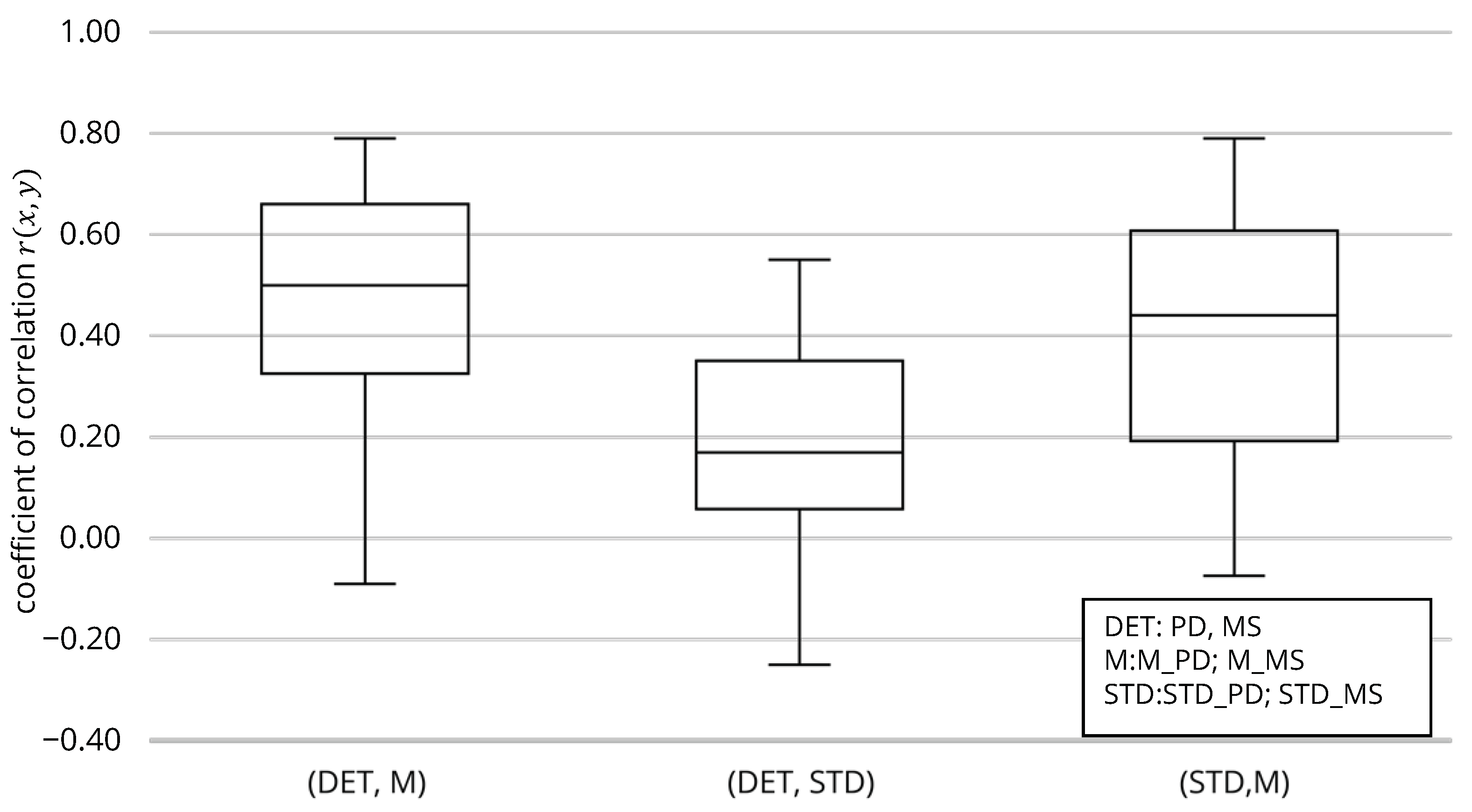
  • We perform a Pareto optimization [40] (pp. 197–199) with the NSGA-III on project level, where the mean and standard deviation of delay and makespan of a single project are considered to evaluate the generated CPRs.
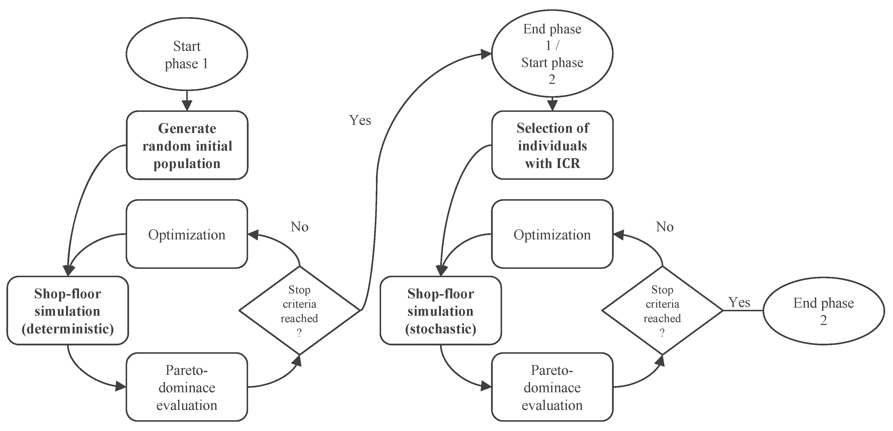
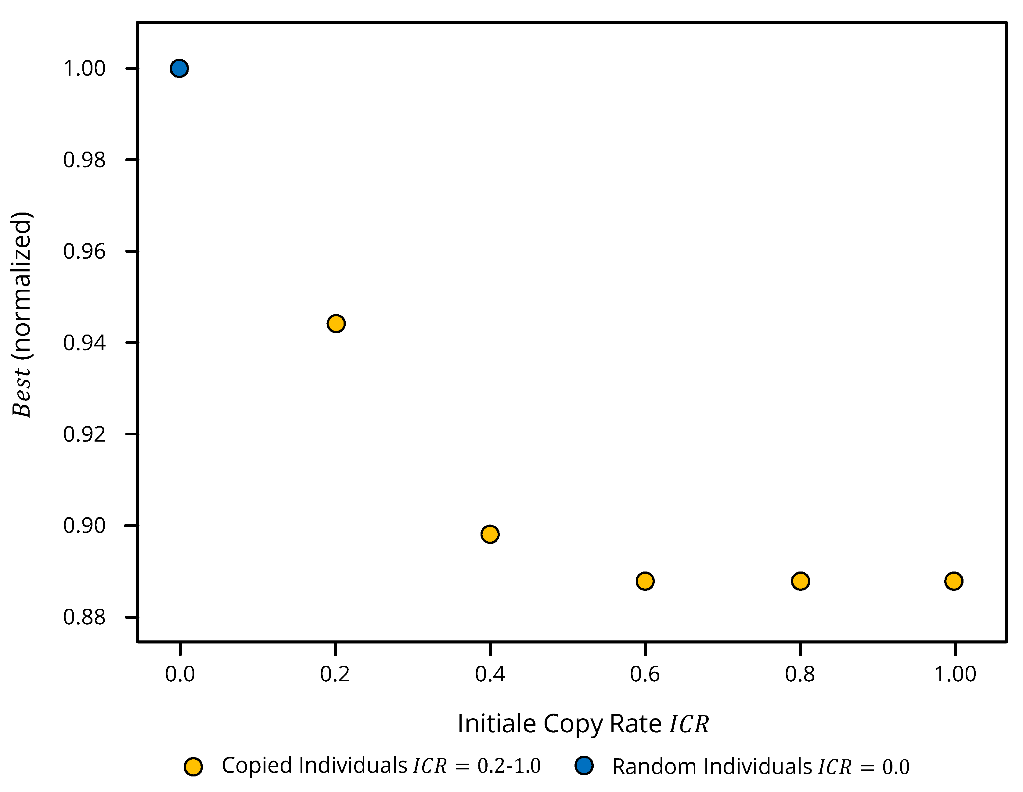
  • A deterministic and stochastic optimization phase takes place for reducing computational effort. For the selection of deterministic solutions, we introduce the parameter Initial Copy Rate (ICR), which indicates how many solutions are copied and how many are randomized.
  • We developed a software framework for generating CPRs and compared results with several different PRs.

3. Model Extensions of the Stochastic RCMPSP

In order to achieve the requirements of the project-specific objectives, a Pareto optimization is aimed as the multi-objective optimization method ( m i n i m i z e ( f 1 ( x ) , f 2 ( x ) , , f z f ( x ) ) with z f > 2 objective functions f y ).
Due to the stochastic influences, it is necessary to evaluate the individual objective values with statistical parameters. A stochastic scenario n is a realized random number of a specific distribution for job processing times (Section 2.1). The mean value and the standard deviation are considered. The mean value is an indicator for optimality of the solution. The standard deviation is an indicator for the robustness of the solution. A low standard deviation means that many solutions are close to the mean value and therefore stochastic influences are better compensated. The following objective functions are set up for the stochastic scenario.
For measuring the tardiness of project i of scenario n, the project delay P D i n is calculated by Equation (1):
f y = P D i n = max 0 , ω J i n f z i
where ω | J | i n is the scheduled finish time of the last job j of project i of the stochastic scenario n and f z i is the determined finish time of project i.
Another objective value is the makespan M S i n , which is calculated by Equation (2):
f y = M S i n = ω J i n α 1 i n
where α 1 i n is the starting time of the first job j of project i of the stochastic scenario n. The following objective functions are set up for statistic evaluation of the stochastic scenarios. Equation (3) calculates the mean of project delay M _ P D i of | N | stochastic scenarios:
f y = M _ P D i = 1 N n N P D i n
Equation (4) calculates the deviation of project delay M _ P D i of | N | stochastic scenarios:
f y = S T D _ P D i = 1 N n N ( P D i n M _ P D i ) 2
The corresponding statistical objective values for makespan M S i are calculated in the same way as Equations (3) and (4) ( S T D _ M S i ; M _ M S i ). Statistical parameters for each objective value are assigned individually ( S T D _ or M _ ) or in combination ( S T D _ and M _ ), so that, in total, six objective functions are considered. For the objective makespan, the objective functions are given as an example. Minimize the average makespan of individual projects M _ M S as in Equation (5):
f = M _ M S = ( M _ M S i , , M _ M S I ) min
Minimize the standard deviation makespan of individual projects S T D _ M S using Equation (6):
f = S T D _ M S = ( S T D _ M S i , , S T D _ M S I ) min
Minimize the average and standard deviation of the makespan of individual projects M _ S T D _ M S using Equation (7):
f = M _ _ S T D _ M S = ( S T D _ M S i , , S T D _ M S I , M _ M S i , , M _ M S I ) min

4. Proposed Algorithm for Generating CPR

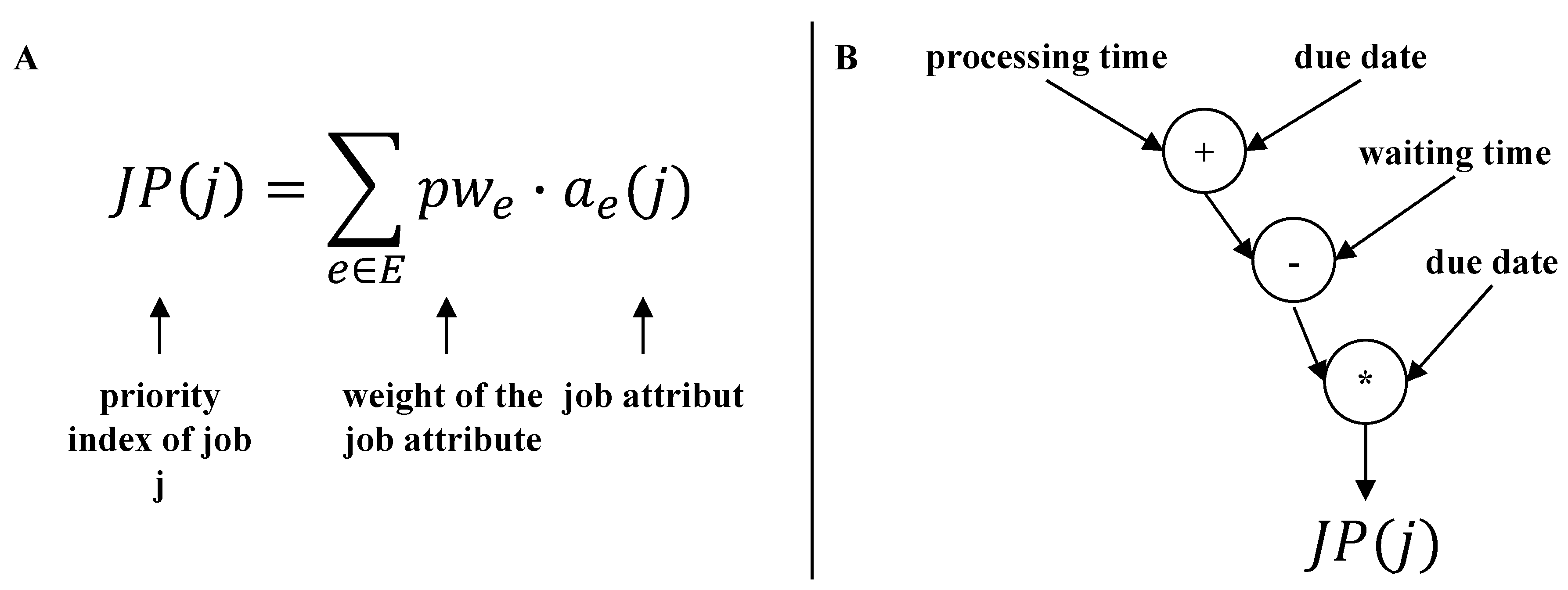
4.1. Representation of CPR

As a sequence heuristic (SH), we use the basic approach of CPRs with weighting factors, the so-called linear representation of CPRs (Figure 2). Job attributes a e are, for example, the expected processing time or the required completion date. The weightings can be determined either by an expert, randomly, or by an algorithm. As an extension to previous research work and in order to meet the requirement of project-specific objective fulfillment, weighting factors p w i e are assigned individually to each project i. Thus, according to the individual objective function f y and project characteristics, individual job attributes a e can be preferred or disadvantaged.
The considered job attributes a e are summarized in the tuple A A :
A A = ( a 1 , , a e ) ,
with e E , where e N [ 1 E ] . A project-specific weight set P S W i is defined as follows and has the same length like A A :
P S W i = ( p w i 1 , , p w i e ) ,
with
e E p w i e = 1 where p w i e R [ 0 , 1 ]
For each job in a queue, the first step is to calculate the individual job priority according to the project-specific weight set and job attribute. Formally, the queue is a list of jobs with corresponding job attributes. Normalizing the values is necessary due to the different dimensions of the job attributes. After calculating the priority, the next step is sorting the jobs in descending order of priority. The job with the highest priority is executed next. Calculation of the job priority J P j i of job j of project i is done with the following equation:
J P j i j i e , m a x J I e = P S W i · A A j i e , m a x J I e = e E p w i e · a e j i e a e m a x J I e
where with j i e is the considered value of attribute a e of the considered job j of project i and m a x J I e is the maximum value of attribute a e of all jobs J I in the considered queue. The job attributes considered were based on locally determined attributes (here, among other things, information is obtained from the examples in MPSPLIB) and are oriented on the used information of the SPR (e.g., processing time, due date, starting time, work remain, and cumulative waiting time).

4.2. Two-Phase Genetic Algorithm for Generating CPRs

The parameterization of the weighting set poses a combinatorial problem with a large solution space. It is not possible to check all individual parameter combinations due to the high computational effort involved. To handle such large search spaces, evolutionary algorithms such as GAs are suitable. With regard to the problem of parameterizing the equation for determining job attributes, the GA corresponds to a hyper-heuristic. Therefore, they are suitable for the problem under consideration. Parallel computing can shorten computation time, especially in stochastic optimization. Computation time increases if the stochastic influences are already taken into account during the training phase. Since there is a correlation between the deterministic and stochastic solutions, we see potential in the combination of deterministic and stochastic training data for saving computation time. If the objective is to use this correlation, i.e., to generate a good quality initial population of solutions for a shorter computation time in the next phase, it is necessary to consider a multitude of deterministic solutions in the stochastic environment. We investigate the quantity and the best solutions for this purpose. Within the scope of the present research, a two-phase algorithm is proposed.
Phase one (Figure 3) starts with an initialization. This means that initial parameters of GA are selected along with the production model (planning task), and it is possible to define the attributes used for the CPRs. Next, initial solutions are generated randomly. Random numbers determine the weightings p w i e of the attributes a e . Based on the defined weightings for the respective attributes, the production is simulated (shop-floor simulation) with deterministic process times. The result is evaluated, and after a negative check of the stop criterion (unchanged objective values after a defined number of iterations), the weightings are changed by the GA. This process continues until the stopping criteria is reached. The result is a set of different weighting variations evaluated with respect to the objective value. In phase two, the corresponding weighting variants from phase one are firstly selected with the parameter initial copy rate I C R . An I C R = 0.2 means that the initial solution for stochastic optimization consists of 20 % copied solutions from the first phase. The other 80 % are random solutions. Then, in accordance with the theory of simulation-based optimization, GA adjusts weights until the stopping criteria is reached. Although the algorithm generated many schedules with different CPRs, the result is only the CPRs with which the best schedules were generated under stochastic conditions. Under stochastic conditions, the objective value will be identical when using this CPRs. The result of the training phase is therefore the result of the test phase.
In accordance with the research aim of project-specific multi-objective optimization, the differentiated evaluation of the quality of solutions (solutions are the project-specific weight sets P S W i , in the context of GA, an individual I n d ) is carried out according to the Pareto dominance concept. Assuming two solution tuples A and B with z f objective functions f y and the goal of minimizing the objective values ( f y ( a ) ; f y ( b ) ) , solution A dominates solution B if f y ( a ) f y ( b ) applies for y = 1 , 2 , , z f and for at least one y f y ( a ) < f y ( b ) .
Based on this rule, all individuals I n d of a population P g e n of generation g e n can be compared in the current scenario. Non-dominated solutions are elements of a non-dominated solution front ( f r o n t = 1 ) . Since there are more than one solution in the Pareto front, we aggregate and normalize the individual objective to an overall objective value as a tiebreaker. The best solution gets the index B e s t . The formation of a new population P g e n + 1 is carried out with the NSGA-III. The algorithm was developed for multi-objective problems with z f > 3 objective functions f y . The entire algorithm for generating the CPRs is called Genetic Algorithm Weighted Sum (GAWS).

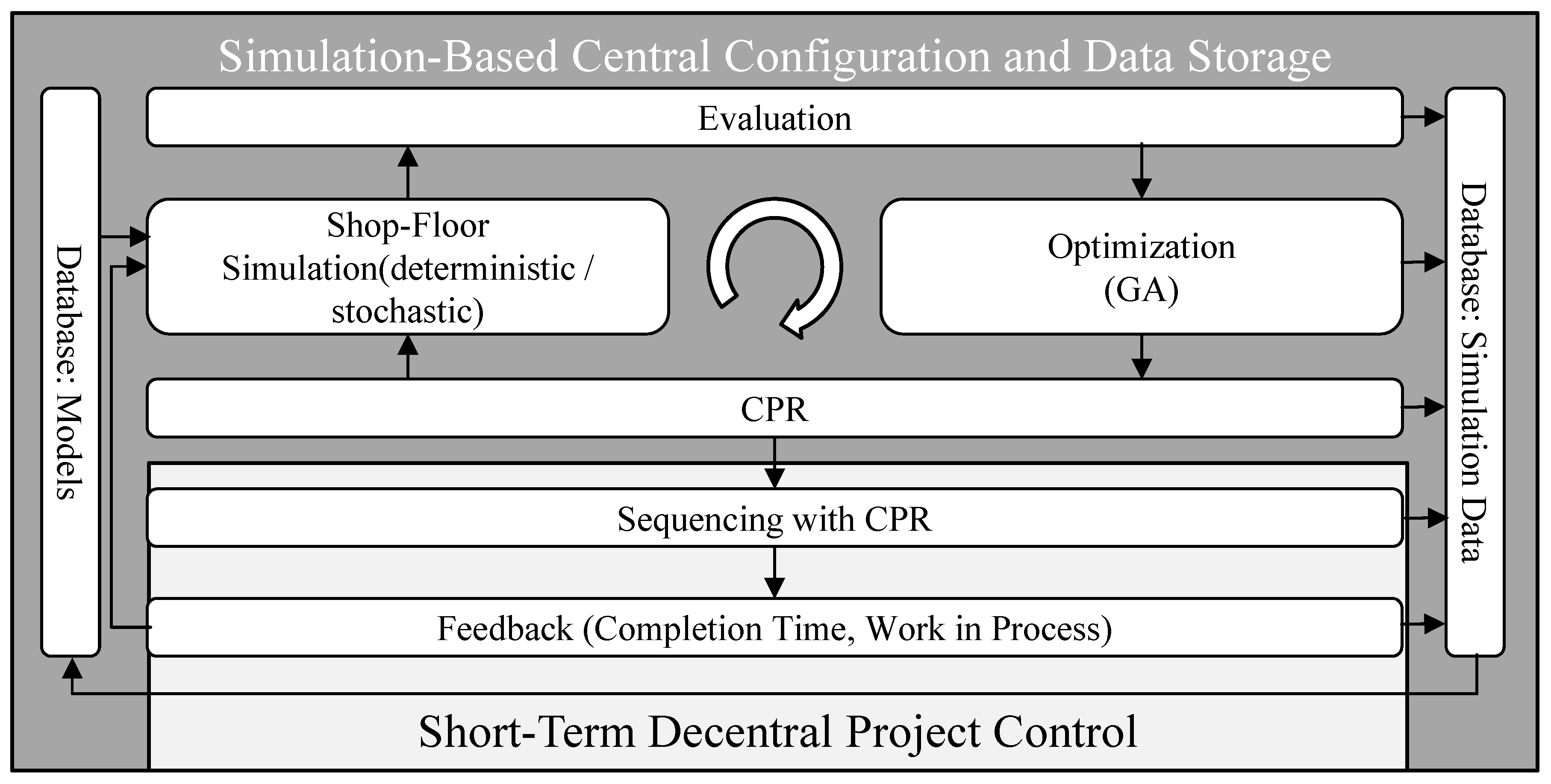
4.3. Overall Concept for Using CPRs and Proposed Software-Framework

The presented concept (Figure 4) for decentralized sequencing is suitable for short-term sequencing at the operation level. For a short-term horizon, SHs are defined by how individual jobs are operatively sequenced on the shop floor. The result is therefore not an implemented schedule by the control system but evolved CPRs that are applied by the control system. The input to generate the CPRs is therefore a defined project pool with jobs or a predefined time horizon. The definition of the input is not part of the analysis but is taken as given in medium-term planning (e.g., MRP-II). Based on a project pool, the proposed algorithm for generating the CPRs is applied. The CPRs are transferred to production resources and applied for the defined validity period. This process is comparable to transfer of the production schedule to actual production. Various options are conceivable for technical implementation: In addition to the transfer to stationary computers at the workstations, the transfer to mobile devices (smartphones and handhelds) is also possible. A possible technical implementation of the CPRs with regard to job identification is for example barcode technology. The barcode contains all information about the projects. The stationary PC or handheld device contains CPRs for determining job priority. New incoming jobs can thus be added to the queue, and if renewable resources become available, the next job to be processed can be determined according to the CPRs. Thus, a rough status regarding finished jobs is known. Moreover, it is possible to share reconfiguration-relevant events (resource failure, etc.) through feedback and to initiate recalculation of CPRs based on the adjusted production parameters.
We developed a software framework based on the Python programming language [41] called PyScOp (Python-Based Scheduling and Optimization Framework) to test the algorithm when generating the project-specific CPRs [42,43]. The developed software framework covers all functionalities from model generation to discrete-event simulation-based optimization and evaluation. To calculate the proposed CPRs in the form of weighting sets, the model is first imported. The standard format of MPSPLIB is used. The next step is parameterization of the model (definition of project-specific objectives) and the algorithm (stop criterion, etc.). With subsequent simulation and optimization, the project-specific CPRs are generated. In addition to the standard function for calculating CPRs, various options for evaluating the performance of the algorithm itself and the CPRs are integrated, which largely correspond to the experiments discussed in Section 5. For technical details, please refer to the method documentation within the software code. The software framework has a graphical user interface for simplified use by third parties. Intended tool tips make it easier for the first user to carry out experiments.

5. Results

5.1. Experiment Design for Concept Evaluation

As mentioned, we use benchmark problems from the MPSPLIB to evaluate the concept. We carried out preliminary investigations to determine the runtime of an optimization run (Intel® Xenon® Gold 6136 with 3.00 GHz CPU and 64 GB RAM). The average optimization takes about 12 h (average from small model | J i | = 30 , | I | = 2 to large model | J i | = 120 , | I | = 5 ). The number of experiments must be limited for this runtime. We chose a two-factor plan as the experimental plan for the model parameters. Each factor is assigned two levels and is combined. The levels should represent a low and a high level. This type of experimental design is chosen if many factors are to be investigated and experiments are highly computation intensive. To avoid process-inherent coincidences, the number of repetitions per single experiment is set to W = 10 [44] (p. 630); [45] (p. 593). The selected models of the MPSPLIB differ in the number of jobs | J i | = 30 and 120, number of projects | I | = 2 and 5, and different instances (network character) i z = 1 and 2, so that a total of 8 models M are considered. The distribution of the process time is considered with c v l o g n o r m = 0.1 and 0.9 . Other parameters are considered to be multifactorial and combined with the mentioned two-factor plan. These parameters are the objective functions f (6 factor stages) and the initial copy rate I C R (6 factor stages). These factor combinations are combined with the number of stochastic scenarios N . Standard values are assumed for the genetic operators by Schmidt et al. [43]. The population size is calculated according to Das et al. [46]. The number of stochastic scenarios for the evaluation of one CPR = GAWS is N = 100 (usually, in Freitag et al. [47], N = 50 , while in Hildebrandt et al. [48], N = 100 ) with n N .

5.2. Comparing Deterministic and Stochastic Solutions

For the comparison between deterministic and stochastic solutions, a deterministic optimization is performed first. Afterwards, the generated deterministic solutions ( f = P D and f = M S ) are tested with stochastic values of the scenarios N . f = M _ P D , f = S T D _ P D , f = M _ M S , and f = S T D _ M S are used as objective functions to evaluate the stochastic influences. The maximum number of generations is g e n = 100 . The deterministic optimization aborts after g e n = 20 generations with an unchanged objective value. E x p a m t = 2 · c v l o g n o r m · 8 M · 6 f · 10 W = 960 experiments were performed. To evaluate the correlation, the Pearson correlation coefficient r ( x , y ) is calculated. For this purpose, the correlation between the deterministic solution ( D E T ) and mean value ( M ) of the stochastic solution, the correlation between the deterministic solution and standard deviation ( S T D ) of the stochastic solution, and the correlation between the mean value ( M ) and standard deviation ( S T D ) of the stochastic solution are calculated. The results are shown in Figure 5 as a boxplot diagram and in Table 1 combined with the mean value and confidence interval k i 0.95 .
A high correlation exists between the deterministic solution ( D E T ) and the mean value of the stochastic solution ( M ) . Furthermore, there is a significant correlation between the mean value ( M ) and the standard deviation of the stochastic solution ( S T D ) . A low correlation exists between the deterministic solution ( D E T ) and the standard deviation of the stochastic solution ( S T D ) . This reinforces the statement that deterministic solutions can be suitable as initial solutions for stochastic optimization. Therefore, setting the parameter initial copy rate I C R is of interest.

5.3. Comparing Computation Effort

In order to evaluate whether the simulation effort and thus the computational effort can be reduced with the presented 2-phase algorithm, a comparison of the simulation effort between the strategy for generating the initial population and the randomized generation of the initial population is necessary. The strategy for optimization of the initial population is called copied in the following, the strategy for the random generation of the initial population is called random. The simulation effort S A I C R to generate the initial population with an initial copy rate of I C R > 0.0 is higher in contrast to the simulation effort of the randomized population S A r a n d with an initial copy rate of I C R = 0.0 . In order to equate the simulation effort S A I C R = S A r a n d , the following assumptions for calculation of the simulation effort are made and demonstrated using a calculation example: The deterministic simulation effort S A d e t for the first phase of the 2-phase algorithm with p o p = 100 , generation amount G A d e t = 100 , and | W | = 10 repetitions is S A d e t = 100,000 ( G A d e t · p o p · | W | ). Selection of the 100 best solutions with respect to the objective value out of 10 repetitions |W| with subsequent stochastic simulation with | N | = 100 scenarios to generate the stochastic initial population leads to a further simulation effort of S A i n i t = 100,000 ( p o p · | N | · | W | ) simulations, so that the total simulation effort is S A I C R = 200,000 ( S A d e t + S A i n i t ). To compare the simulation effort, for example, more randomized solutions can be generated S A i n i t = S A r a n d = 200 p o p · 100 | N | · 10 | W | = 200,000 . Another possibility is to leave the population size p o p unchanged at p o p = 100 S A i n i t = 100 p o p · 100 | N | · 10 | W | = 100,000 and additionally to perform a generation step G A s t o c h = 1 within the framework of stochastic optimization at S A s t o c h = 1 G A s t o c h · 100 p o p · 100 | N | · 10 | W | = 100,000, so that the simulation effort with the randomized initial population also corresponds to S A r a n d = 200,000 ( S A i n i t + S A s t o c h ). The latter option was chosen for comparison purposes, since it also uses the mode of action of the genetic algorithm, which requires a certain calculation time and thus makes the results more comparable. Figure 6 illustrates the performance of the different strategies for generating the initial population (randomized I C R = 0.0 and copied ICR = 0.2–1.0).
One possibility to evaluate the effectiveness of a copied initial population ICR = 0.2–1.0 is to compare the objective fulfillment of the best solution B e s t per experiment (Figure 7). A condensed evaluation is the relative frequency with which an I C R achieves the best value for the objective value B e s t per individual experiment. Of the 96 possible individual experiments ( 2 V a r K l o g n o r m · 8 M · 6 f ) , a copied initial population (ICR = 0.2–1.0) achieves the best objective value B e s t in 79.17 % of the individual experiments. In 20.83 % of the experiments, a randomized initial population achieves the best objective value ( I C R = 0.0 ) . The initial copy rate of I C R = 0.4 and I C R = 0.6 is more often used to achieve the best objective value B e s t ( 22.5 % ) than the initial copy rates I C R = 0.2 , 0.8 , and 1.0 ( 12 % ) . The following conclusions can be drawn from the distribution of the frequency:
  • An optimization of the initial population does not necessarily lead to the best result with respect to the objective value B e s t .
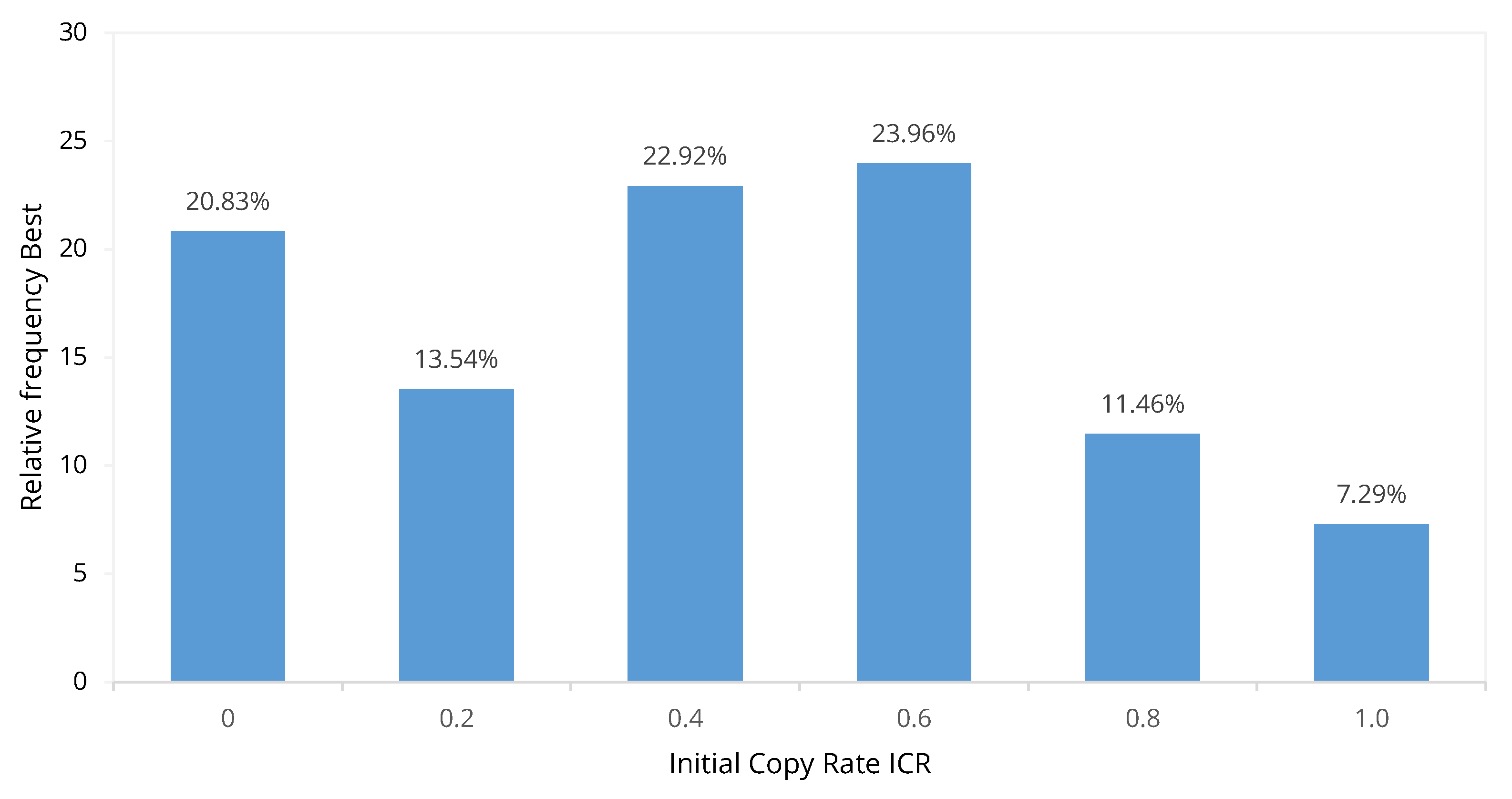
  • A low and a too high initial copy rate lead less frequently to the best objective value B e s t . Therefore, it can be concluded that either too many randomized solutions ( I C R < 0.4 ) or too many copied solutions ( I C R > 0.6 ) do not sufficiently represent the correlation between deterministic and stochastic solution and that, therefore, for a diverse initial population, an equal ratio of copied and randomized solutions is most promising.
The relative saving B e s t r e l between the copied population (ICR = 0.2, 0.4, 0.6, 0.8 and 1.0) compared to the randomized population ( I C R = 0.0 ) is used to evaluate the performance of the initial copy rate I C R .
A positive value B e s t r e l means a saving; a negative value B e s t r e l is a loss. B e s t r e l % is calculated by the following:
B e s t r e l ( % ) = 1 B e s t ( I C R = 0.2 ; 0.4 ; 0.6 ; 0.8 ; 1.0 ) B e s t ( I C R = 0.0 ) · 100
With increasing initial copy rate I C R , the range of the relative saving potential B e s t r e l increases (Table 2). From this, it can be concluded that, with initial copy rate I C R , the saving potential B e s t r e l fluctuates significantly more and can be predicted less reliably. Thus, the initial copy rate I C R should be selected in such a way that the savings are maximized on average x ¯ ( % ) with a high probability k i 0.95 ( % ) . When using the initial copy rate of ICR = 0.2–1.0, better results B e s t r e l are obtained for 58.3 % ( I C R = 1.0 ) to 69.7 % ( I C R = 0.4 ) of the considered individual experiments than with an initial copy rate of I C R = 0.0 . If the best initial copy rate I C R B e s t was always selected, the results B e s t r e l will be better in 79.17 % of the individual experiments compared to randomized solutions ( I C R = 1.0 ) . In contrast, the results B e s t r e l will be worse in 55.2 % of the individual experiments if the worst initial copy rate I C R W o r s t was selected. The average x ¯ best saving B e s t r e l is achieved with an initial copy rate I C R = 0.6 ( x ¯ = 0.42 % ) , and the median x ˜ best saving B e s t r e l is achieved with an initial copy rate I C R = 0.4 ( x ˜ = 0.46 % ) . These values should not be regarded as too low, since, as will be examined in Section 5.4, the overall optimization potential is approximately 4 % . With both I C R = 0.4 and I C R = 0.6 , the confidence interval is k i 0.95 = ± 0.49 % . Thus, there is no clear recommendation for the selection of an initial copy rate I C R , but I C R = 0.4 or I C R = 0.6 should be preferred. The following experiments uses I C R = 0.6 .

5.4. Evaluation of the Overall Quality of The Algorithm

To evaluate the performance of the overall concept, the objective value of the initial population is compared with the objective value of the last population of the optimization run. The maximum number of generations for deterministic and stochastic optimization is g e n = 100 with a stop criterion of g e n = 20 generations. The number of experiments is similar to that mentioned in Section 5.3. Since the results of the repetitions W do not differ significantly, W is set to W = 1 for the next experiments. With a coefficient of variation of c v l o g n o r m = 0.9 , the optimization potential is between 0–1% in about 50 % of the experiments (Figure 8). For the remaining experiments, an optimization potential between 1–5% is achieved.
A higher optimization potential is achieved with a coefficient of variation of c v l o g n o r m = 0.1 (Figure 9). In about 50 % of the experiments, the optimization potential is higher than 5 % . It is remarkable that, in about 15 % of the experiments, the optimization potential is between 15–30%. This represents that the optimization potential decreases with large stochastic influences, which represents that the actual process time deviates significantly from the expected value and that the solution is highly random. This corresponds almost to a complete lack of process knowledge so that an online optimization is probably more effective.
If we have a detailed look at the parameters (Figure 10), we see that there is a better improvement in general for the objective function project delay toward makespan. The model parameters have no significant influence. The influence of the coefficient of variation of the distribution is significant. In the median, an improvement of approximately 4 % occurs independently of the parameters.

5.5. Comparison with Standard Priority Rules

For evaluation of the presented algorithm, we compare the performance of the P R = G A W S with the P R = S P R on 25 models M from the MPSPLIB, which essentially differ from the previously considered models by the instances. The experiments vary with respect to the coefficient of variance c v l o g n o r m and the objective function f. The parameter initial copy rate I C R is still considered I C R = 0.6 . The parameters of the GA are the same as in Section 5.4. Common SPRs serve as comparison criteria [49,50].
The presented algorithm achieves under stochastic influences without Pareto criterion in 50 % better results than the considered SPR (Figure 11). The second best SPR MWRK (Most Work Remaining) achieves better results in 12 % of the experiments, the third best SPR EDD (Earliest Due Date) achieves better results in 8 % of the experiments, and the fourth best SPR FIFO achieves better results in 6 % of the experiments. The remaining SPRs achieve the best results in 1 % on average.
Looking at the three best PRs (GAWS, MWRK, and EDD) in Figure 12, it can be seen that all three PRs are represented on all ranks, with rank = 1 being the best PR and rank = 20 being the worst PR. GAWS is 95 % among the 10 best PRs (sum of the relative frequency of GAWS from r a n k = 1 to r a n k = 10 ). SPR EDD is among the ten best SPRs in 70 % of the experiments (sum of the relative frequency of EDD from r a n k = 1 to r a n k = 5 ). It is remarkable that the MWRK comes last ( r a n k = 20 ) in almost 10 % of the experiments.
In the following, the saving potential is quantified if the CPR GAWS ranks first (Table 3). On average, there is a saving of 3.3 % compared to r a n k = 2 regarding the objective value. Compared to the average performance, there is a saving of 10.8 % , and compared to the worst SPR, there is a saving of about 25 % .
If CPR GAWS does not occupy rank = 1, there is an average loss compared to r a n k = 1 of 10.6 % regarding the objective value (Table 4). Compared to the medium performance of the other SPRs, an average saving of 3.63 % is still achieved. Comparing CPR GAWS to the worst SPR, an average saving of 18.9 % is achieved. In summary, the presented CPR can achieve an average improvement over a randomly selected SPR.
For complete evaluation of the presented CPR GAWS, it is necessary to assess the fulfillment of individual project objectives according to the Pareto criterion (Table 5). For this purpose, the solutions are divided into solution fronts (Section 4.2). CPR GAWS is on average in 90 % of the experiments in the first front. There are no significant deviations when considering individual parameters. The only difference shows the parameter instance i z . A performance analysis of the other SPRs shows that no SPR dominates another SPR with regard to its occurrence in the first front. The SPR FIFO is often in the first front. As far as frequency is concerned, no other SPR comes close to the presented CPR GAWS. This shows the real potential of CPR GAWS.

6. Conclusions and Outlook

In this paper, we present and study a 2-phase genetic algorithm for the efficient generation of project-specific composite priority rules for short-term production control of the stochastic resource-constrained multi-project scheduling problem. Computational results with our presented discrete-event simulation-framework PyScOp show that, with the same simulation effort, the proposed algorithm achieves better initial solutions compared to complete randomly generated initial solutions on average. The best initial population is based on half copied best and half randomly selected solutions. The experiments also show that, with our algorithm, the objective fulfillment compared to priority rules used in practice is much better. Our solutions are in 90 % of the experiments in the Pareto front. The best priority rule FIFO is in about 65 % of the experiments in the Pareto front. All experiments show that the performance of the algorithm depends on the model parameter.
We see further research in the parameter optimization of the GA to improve the generated composite priority rules. The computational effort can be further reduced if additional strategies for generating the initial population are applied. This includes generation of the start solution with known priority rules or with solutions from similar models. In general, the model-attribute-objective effects need to be further analyzed in order to set model-dependent parameters that can improve both computation time and objective values.

Author Contributions

Conceptualization, M.K.; methodology, M.K.; software, M.K.; writing—original draft preparation, M.K.; writing—review and editing, Michael Völker and T.S.; visualization, M.K.; supervision, M.V. and T.S.; project administration, T.S. All authors have read and agreed to the published version of the manuscript.

Funding

This work is funded by the German Research Foundation (DFG) within the projects Simulation-based generation of robust heuristics for self-control of manual production processes: A hybrid approach on the way to industry 4.0 (Project ID 418727532) https://gepris.dfg.de/gepris/projekt/418727532 and Sim4Pep (Project ID 439188616) https://gepris.dfg.de/gepris/projekt/439188616.

Conflicts of Interest

The authors declare no conflict of interest.

Abbreviations

The following abbreviations are used in this manuscript:
APSAdvanced Panning and Scheduling
CDRComposite Dispatching Rule
CPRComposite Priority Rule
CPPSCyber Physical Production System
GAGenetic Algorithm
GAWSGenetic Algorithm Weighted Sum
ICRInitial Copy Rate
MESManufacturing Execution System
MPSPLIBMulti-Project Scheduling Library
PPCProject Planning and Control
PSPLIBProject Scheduling Linrary
RCPSPResource Constrained Project Scheduling Problem
SHSequencing Heuristic
SPRSimple Priority Rules
SRCMPSPStochastic Resource Constrained Multi-Project Scheduling Problem

References

  1. Bischoff, J.; Taphorn, C.; Wolter, D.; Braun, N.; Fellbaum, M.; Goloverov, A.; Ludwig, S.; Hegmanns, T.; Prasse, C.; Henke, M.; et al. Erschließen der Potenziale der Anwendung von Industrie 4.0 im Mittelstand; BMWi: Berlin, Germany, 2015. [Google Scholar]
  2. Huber, W. Industrie 4.0 Kompakt—Wie Technologien Unsere Wirtschaft und Unsere Unternehmen Verändern; Springer Fachmedien Wiesbaden: Wiesbaden, Germany, 2018. [Google Scholar] [CrossRef]
  3. Lödding, H. Verfahren der Fertigungssteuerung: Grundlagen, Beschreibung, Konfiguration; Springer: Berlin/Heidelberg, Germany, 2016. [Google Scholar]
  4. Glonegger, M. Berücksichtigung Menschlicher Leistungsschwankungen bei der Planung von Variantenfließ-Montagesystemen; Forschungsberichte IWB; Utz, Herbert: München, Germany, 2014; Volume 292. [Google Scholar]
  5. Marczinski, G. Einsatzgebiete von ERP-, APS- und MES-Lösungen. ERP Manag. 2008, 2008, 62–64. [Google Scholar]
  6. Niehus, M.R. Adaptive Produktionssteuerung für Werkstattfertigungssysteme durch Fertigungsbegleitende Reihenfolgebildung. Ph.D. Thesis, Technische Universität München, München, Germany, 2016. [Google Scholar]
  7. Hansmann, K.W. Industrielles Management; 8., völlig überarb. und erw. aufl. ed.; Oldenbourg: München, Germany, 2006. [Google Scholar]
  8. Nyhuis, P.; Mayer, J.; Kuprat, T. Die Bedeutung von Industrie 4.0 als Enabler für logistische Modelle. In Industrie 4.0; Kersten, W., Ed.; Schriftenreihe der Hochschulgruppe für Arbeits- und Betriebsorganisation e.V. (HAB); Gito: Berlin, Germany, 2014; pp. 79–100. [Google Scholar]
  9. Peßl, E. Digitale Produktion: Studie über Status, Hemmnisse und Anforderungen österreichischer Produzierender Klein- und Mittelunternehmen und Analyse der Software-Hersteller von MES-Systemen; Inst. Industrial Management/Industriewirtschaft FH JOANNEUM Kapfenberg: Kapfenberg, Austria, 2013. [Google Scholar]
  10. Branke, J.; Nguyen, S.; Pickardt, C.W.; Zhang, M. Automated Design of Production Scheduling Heuristics: A Review. IEEE Trans. Evol. Comput. 2016, 20, 110–124. [Google Scholar] [CrossRef] [Green Version]
  11. Hildebrandt, T.; Heger, J.; Scholz-Reiter, B. Towards improved dispatching rules for complex shop floor scenarios. In Proceedings of the 12th Annual Conference on Genetic and Evolutionary Computation; Pelikan, M., Branke, J., Eds.; ACM: New York, NY, USA, 2010; pp. 257–264. [Google Scholar] [CrossRef]
  12. Pritsker, A.A.B.; Waiters, L.J.; Wolfe, P.M. Multiproject Scheduling with Limited Resources: A Zero-One Programming Approach. Manag. Sci. 1969, 16, 93–108. [Google Scholar] [CrossRef] [Green Version]
  13. Lova, A.; Tormos, P. Analysis of Scheduling Schemes and Heuristic Rules Performance in Resource-Constrained Multiproject Scheduling. Ann. Oper. Res. 2001, 102, 263–286. [Google Scholar] [CrossRef]
  14. Confessore, G.; Giordani, S.; Rismondo, S. A market-based multi-agent system model for decentralized multi-project scheduling. Ann. Oper. Res. 2007, 150, 115–135. [Google Scholar] [CrossRef]
  15. Homberger, J. A multi-agent system for the decentralized resource-constrained multi-project scheduling problem. Int. Trans. Oper. Res. 2007, 14, 565–589. [Google Scholar] [CrossRef]
  16. Homberger, J. MPSPLIB: Multi Project Scheduling Problem Library. Hochschule für Technik Stuttgart. 2008. Available online: www.mpsplib.com (accessed on 17 October 2020).
  17. Kolisch, R.; Sprecher, A. PSPLIB—A project scheduling problem library. Eur. J. Oper. Res. 1996, 96, 205–216. [Google Scholar] [CrossRef] [Green Version]
  18. Blazewicz, J.; Lenstra, J.; Rinnooy Kan, A. Scheduling subject to resource constraints: Classification and complexity. Discret. Appl. Math. 1983, 5, 11–24. [Google Scholar] [CrossRef] [Green Version]
  19. Ballestín, F. When it is worthwhile to work with the stochastic RCPSP? J. Sched. 2007, 10, 153–166. [Google Scholar] [CrossRef]
  20. Kolisch, R.; Hartmann, S. Heuristic Algorithms for the Resource-Constrained Project Scheduling Problem: Classification and Computational Analysis. In Project Scheduling: Recent Models, Algorithms and Applications; Węglarz, J., Ed.; Springer US: Boston, MA, USA, 1999; pp. 147–178. [Google Scholar] [CrossRef]
  21. März, L.; Krug, W.; Rose, O.; Weigert, G. Simulation und Optimierung in Produktion und Logistik; Springer: Berlin, Germany, 2011; Volume 1. [Google Scholar] [CrossRef]
  22. Herroelen, W. Project Scheduling—Theory and Practice. Prod. Oper. Manag. 2005, 14, 413–432. [Google Scholar] [CrossRef] [Green Version]
  23. Schade, K. Stochastische Optimierung. In Stochastische Optimierung; Schade, K., Ed.; Stochastic Programming, Vieweg+Teubner: Wiesbaden, Germany, 2012; pp. 45–72. [Google Scholar] [CrossRef]
  24. Ashtiani, B.; Leus, R.; Aryanezhad, M.B. A Novel Class of Scheduling Policies for the Stochastic Resource-Constrained Project Scheduling Problem. SSRN Electron. J. 2008. [Google Scholar] [CrossRef] [Green Version]
  25. Stork, F. Stochastic Resource-Constrained Project Scheduling. Ph.D. Thesis, Technische Universitat Berlin, Berlin, Germany, 2001. [Google Scholar] [CrossRef]
  26. Ashtiani, B.; Leus, R.; Aryanezhad, M.B. New competitive results for the stochastic resource-constrained project scheduling problem: Exploring the benefits of pre-processing. J. Sched. 2011, 14, 157–171. [Google Scholar] [CrossRef]
  27. Deb, K.; Jain, H. An Evolutionary Many-Objective Optimization Algorithm Using Reference-Point-Based Nondominated Sorting Approach, Part I: Solving Problems With Box Constraints. IEEE Trans. Evol. Comput. 2014, 18, 577–601. [Google Scholar] [CrossRef]
  28. Kück, M.; Broda, E.; Freitag, M.; Hildebrandt, T.; Frazzon, E.M. Towards adaptive simulation-based optimization to select individual dispatching rules for production control. In Proceedings of the 2017 Winter Simulation Conference (WSC), Las Vegas, NV, USA, 3–6 December 2017; pp. 3852–3863. [Google Scholar] [CrossRef]
  29. Grundstein, S.; Freitag, M.; Scholz-Reiter, B. A new method for autonomous control of complex job shops—Integrating order release, sequencing and capacity control to meet due dates. J. Manuf. Syst. 2017, 42, 11–28. [Google Scholar] [CrossRef]
  30. Fink, A.; Homberger, J. Decentralized Multi-Project Scheduling. In Handbook on Project Management and Scheduling; Schwindt, C., Zimmermann, J., Eds.; Springer International Publishing: Cham, Switzerland, 2015; Volume 1, pp. 685–706. [Google Scholar]
  31. Chand, S.; Singh, H.; Ray, T. Evolving heuristics for the resource constrained project scheduling problem with dynamic resource disruptions. Swarm Evol. Comput. 2019, 44, 897–912. [Google Scholar] [CrossRef]
  32. Hildebrandt, T.; Freitag, M. Bessere Prioritätsregeln für komplexe Produktionssysteme mittels multi-kriterieller simulationsbasierter Optimierung. In Simulation in Production and Logistics 2015; Rabe, M., Clausen, U., Eds.; Fraunhofer Verlag: Stuttgart, Germany, 2015; pp. 309–318. [Google Scholar]
  33. Branke, J.; Hildebrandt, T.; Scholz-Reiter, B. Hyper-heuristic Evolution of Dispatching Rules: A Comparison of Rule Representations. Evol. Comput. 2015, 23, 249–277. [Google Scholar] [CrossRef]
  34. Nguyen, S.; Zhang, M.; Tan, K.C. Surrogate-Assisted Genetic Programming With Simplified Models for Automated Design of Dispatching Rules. IEEE Trans. Cybern. 2017, 47, 2951–2965. [Google Scholar] [CrossRef]
  35. Jorapur, V.S.; Puranik, V.S.; Deshpande, A.S.; Sharma, M. A Promising Initial Population Based Genetic Algorithm for Job Shop Scheduling Problem. J. Softw. Eng. Appl. 2016, 9, 208–214. [Google Scholar] [CrossRef] [Green Version]
  36. Werner, F. A Survey of Genetic Algorithms for Shop Scheduling Problems. In Heuristics: Theory and Application; Siar, P., Ed.; Nova Science Publishers: Hauppauge, NY, USA, 2013; pp. 161–222. [Google Scholar]
  37. Nguyen, S.; Zhang, M.; Johnston, M.; Tan, K.C. Automatic Design of Scheduling Policies for Dynamic Multi-objective Job Shop Scheduling via Cooperative Coevolution Genetic Programming. IEEE Trans. Evol. Comput. 2014, 18, 193–208. [Google Scholar] [CrossRef]
  38. Nguyen, S.; Zhang, M.; Johnston, M.; Tan, K.C. A Computational Study of Representations in Genetic Programming to Evolve Dispatching Rules for the Job Shop Scheduling Problem. IEEE Trans. Evol. Comput. 2013, 17, 621–639. [Google Scholar] [CrossRef]
  39. Omar, M.; Baharum, A.; Hasan, Y. A job-shop scheduling problem (JSSP) using genetic algorithm (GA). In Proceedings of the 2nd im TG T Regional Conference, Penang, Malaysia, 13–15 June 2006. [Google Scholar]
  40. Goldberg, D.E. Genetic Algorithm in Search, Optimization, and Machine Learning; Addison-Wesley: Reading, MA, USA, 1989; Volume XIII. [Google Scholar]
  41. Python Software Foundation. Python. 2019. Available online: www.python.org (accessed on 17 October 2020).
  42. Kühn, M. PyScOp. 2019. Available online: https://tlscm.mw.tu-dresden.de/scm/git/PyScOp_2.0 (accessed on 17 October 2020).
  43. Schmidt, T.; Kühn, M.; Genßler, P.R. Design of Project-oriented Calculation Models for Job Priorities by Using a Customized Genetic Algorithm. In Simulation in Produktion und Logistik 2017; Wenzel, S., Peter, T., Eds.; Kassel University Press: Kassel, Germany, 2017; pp. 99–108. [Google Scholar]
  44. Law, A.M.; Kelton, W.D. Simulation Modeling and Analysis, 3rd ed.; internat. ed., [nachdr.] ed.; McGraw-Hill Series in Industrial Engineering und Management Science; McGraw-Hill: Boston, MA, USA, 2000. [Google Scholar]
  45. Sexton, R.S.; Dorsey, R.E.; Johnson, J.D. Optimization of neural networks: A comparative analysis of the genetic algorithm and simulated annealing. Eur. J. Oper. Res. 1999, 114, 589–601. [Google Scholar] [CrossRef]
  46. Das, I.; Dennis, J.E. Normal-Boundary Intersection: A New Method for Generating the Pareto Surface in Nonlinear Multicriteria Optimization Problems. SIAM J. Optim. 1998, 8, 631–657. [Google Scholar] [CrossRef] [Green Version]
  47. Freitag, M.; Hildebrandt, T. Automatic design of scheduling rules for complex manufacturing systems by multi-objective simulation-based optimization. CIRP Ann. 2016, 65, 433–436. [Google Scholar] [CrossRef]
  48. Hildebrandt, T.; Branke, J. On Using Surrogates with Genetic Programming. Evol. Comput. 2015, 23, 343–367. [Google Scholar] [CrossRef]
  49. Haupt, R. A survey of priority rule-based scheduling. Spektrum 1989, 11, 3–16. [Google Scholar] [CrossRef]
  50. Vanhoucke, M. Integrated Project Management Sourcebook; Springer International Publishing: Cham, Switzerland, 2016. [Google Scholar] [CrossRef]
Figure 1. Example of job processing time deviations for a type representative in individual furniture assembly.
Algorithms 13 00337 g001
Figure 2. Combined Priority Rules (CPRs): (A) parameter-based representation and (B) grammar-based representation.
Algorithms 13 00337 g002
Figure 3. Two-phase genetic algorithm.
Algorithms 13 00337 g003
Figure 4. Concept hybrid Project Planning and Control (PPC).
Algorithms 13 00337 g004
Figure 5. Boxplot correlation between the deterministic ( D E T ) and stochastic ( S T D , M ) solutions.
Algorithms 13 00337 g005
Figure 6. Example of how the initial copy rate works; worst value: B e s t = 1.00 .
Algorithms 13 00337 g006
Figure 7. Comparison frequency B e s t between random and copied initial solutions.
Algorithms 13 00337 g007
Figure 8. Performance of the genetic algorithm: comparison between best value initial population and best value last generation of optimization c v l o g n o r m = 0.9 .
Algorithms 13 00337 g008
Figure 9. Performance of the genetic algorithm: comparison between best value initial population and best value last generation of optimization c v l o g n o r m = 0.1 .
Algorithms 13 00337 g009
Figure 10. Performance of the proposed algorithm depending on the single parameters.
Algorithms 13 00337 g010
Figure 11. Performance of the proposed algorithm compared to Standard Priority Rules (SPRs): M W R K : Most Work Remaining; E D D : Earliest Due Date; F I F O : First In First Out; M A X I S : Maximum Immediate (Direct) Successors; M A X R R : Maximum Resource Request; L I F O : Last In First Out; L W R K : Least Work Remaining; C R : Critical Ration; N C R : None Critical Ratio; L D D : Least Due Date; L W T : Longest Wait Time; M S L K : Minimum Slack; M A X N W : Maximum Total Successors; M I N I S : Minimum Immediate (Direct) Successors; L P T : Longest Processing Time; S W T : Shortest Wait Time (cumulative); N C R : None Critical Ration; M I N R R : Minimal Resource Request.
Algorithms 13 00337 g011
Figure 12. Comparison of the performance of the three priority rules.
Algorithms 13 00337 g012
Table 1. Statistical analysis coefficient of correlation.
r ( x , y ) x ¯ k i 0.95
D E T , M 0.47±0.08
D E T , S T D 0.18±0.07
S T D , M 0.34±0.08
Table 2. Relative saving potential initial copy rate for generating the copied population compared to randomized population.
Statistic 0.2 0.4 0.6 0.8 1.0 0.2–1.0BestWorst
A n t ( % ) 66.669.764.662.558.366.479.1755.2
x ¯ ( % ) 0.280.390.420.260.050.260.66−0.37
x ˜ ( % ) 0.370.460.440.410.320.400.580.22
σ ( % ) 2.202.422.402.593.152.552.303.06
k i 0.95 ( % ) ±0.45±049±0.49±0.53±0.64±0.52±0.47±0.62
Table 3. Improvement with GAWS = rank 1.
Comparing GAWS Rank = 1 to
StatisticRank 2MW RankRank 20
x ¯ ( % ) 3.3110.8224.86
x ˜ ( % ) 2.668.4917.64
σ ( % ) 2.887.5620.65
k i 0.95 (%)±0.46±1.20±3.27
Table 4. Deterioration with GAWS ≠ Rank 1.
Comparing GAWS Rank ≠ 1 to
StatisticRank 2MW RankRank 20
x ¯ ( % ) −10.603.6318.90
x ˜ ( % ) −3.222.9114.68
σ ( % ) 19.155.4315.66
k i 0.95 (%)±3.03±0.86±2.48
Table 5. Comparison of objective fulfillment with Pareto criterion.
FilterGAWS = 1st Front (%)2nd Best PR = 1st Front2nd Best PR = 1st Front (%)
All experiments 91FIFO65
cv lognorm = 0.195FIFO61
cv lognorm = 0.988FIFO69
M _ PD 94FIFO74
STD _ PD 90MSLK42
M _ PD _ STD _ PD 92FIFO86
M _ MS 92FIFO72
STD _ MS 82LWRK42
M _ MS _ STD _ MS 98FIFO88
| I | = 2 89FIFO55
| I | = 5 95MAX_NW88
| J i | = 30 95MAX_NW64
J i | = 120 89FIFO71
iz = 1 77FIFO72
iz = 2 100MWRK58
Publisher’s Note: MDPI stays neutral with regard to jurisdictional claims in published maps and institutional affiliations.

