Investigating Social Contextual Factors in Remaining-Time Predictive Process Monitoring—A Survival Analysis Approach


Abstract
1. Introduction
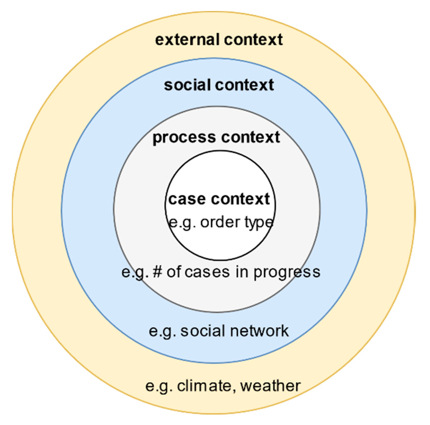
- Case context: the properties or attributes of a case.
- Process context: similar cases that may be competing for the same resources.
- Social context: the way human resources collaborate in an organisation to work on the process of interest.
- External context: factors in the broader ecosystem that impacts the process, e.g., weather, legislation, and location.
2. Materials and Methods
2.1. Definitions
2.1.1. Event, Traces and Event Logs
2.1.2. Survival Functions and Social Networks
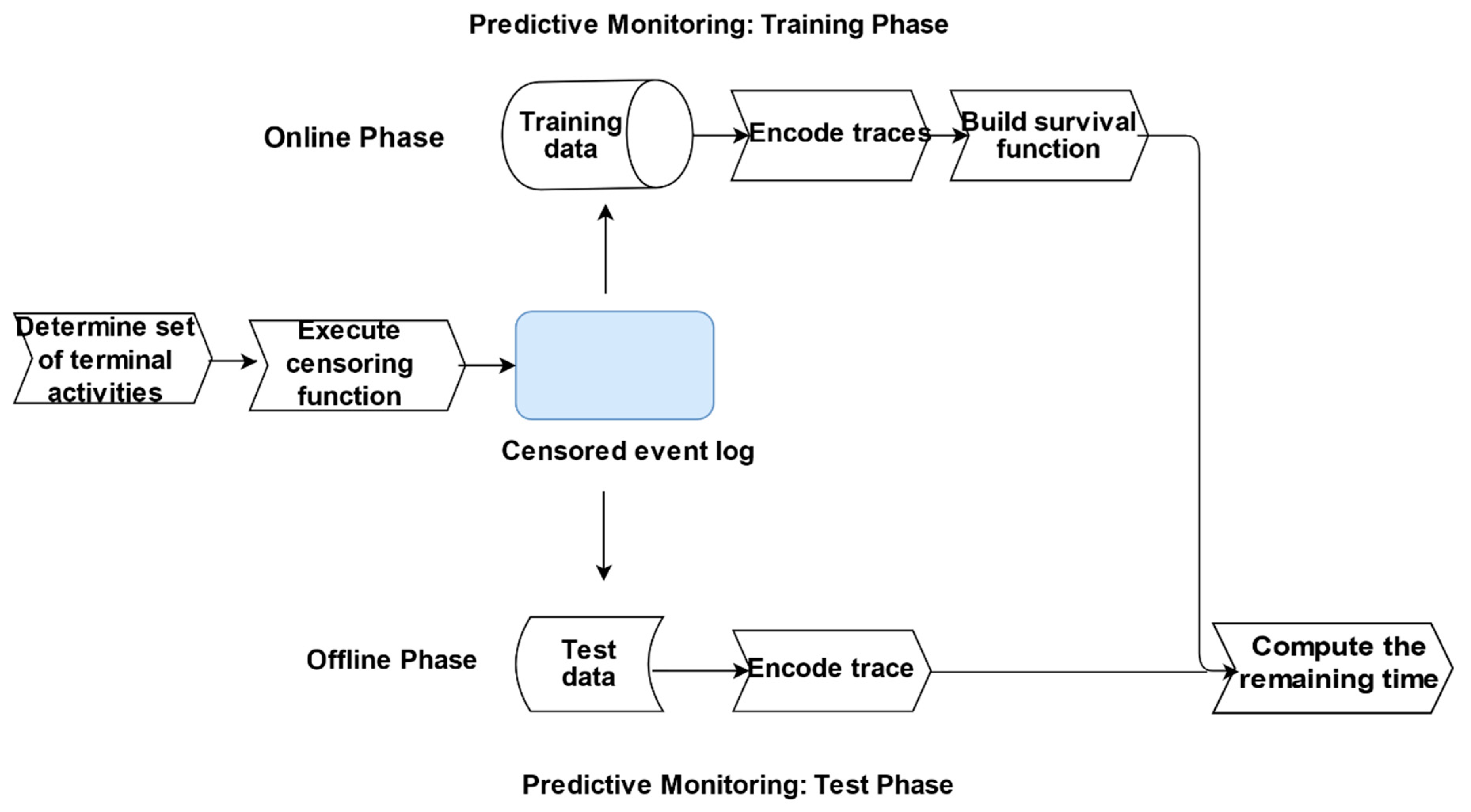
2.2. Overview
2.3. Pre-Processing
2.4. Predictive Monitoring
| Algorithm 1 Survival Algorithm. | |
| Input: | An event log L over some trace universe σ with the associated feature elapsed time τela, cycle time τcyc, a target measure remaining time τrem, a set of terminal activity labels (T), an estimation quantile q and a survival analysis (SURV) method |
| Output: | A Survival Analysis predictive model (SA-PM) for L |
| 1 | Associate a binary variable #censored(σ) with each trace σ ϵ L using #activity(en), T (see definition 3) |
| 2 | Encode each trace using a suitable encoding function |
| 3 | Induce a survival function sa-pm out of L using method SURV {#censored(σi), # cycle time(σi) …..# attributen(σi)} as input value |
| 4 | Let σ1… σn denote each trace |
| 5 | For each σi do |
| 6 | Estimate the cycle time τi.cyc_pred for each trace from sa-pm utilising q |
| 7 | Estimate the remaining time for each trace τi.rem_pred: τi.cyc_pred − τela |
| 8 | End |
| 9 | Return c {τrem_pred1……. τrem_predn} |
2.5. Evaluation
2.5.1. Datasets
2.5.2. Experimental Setup
3. Results
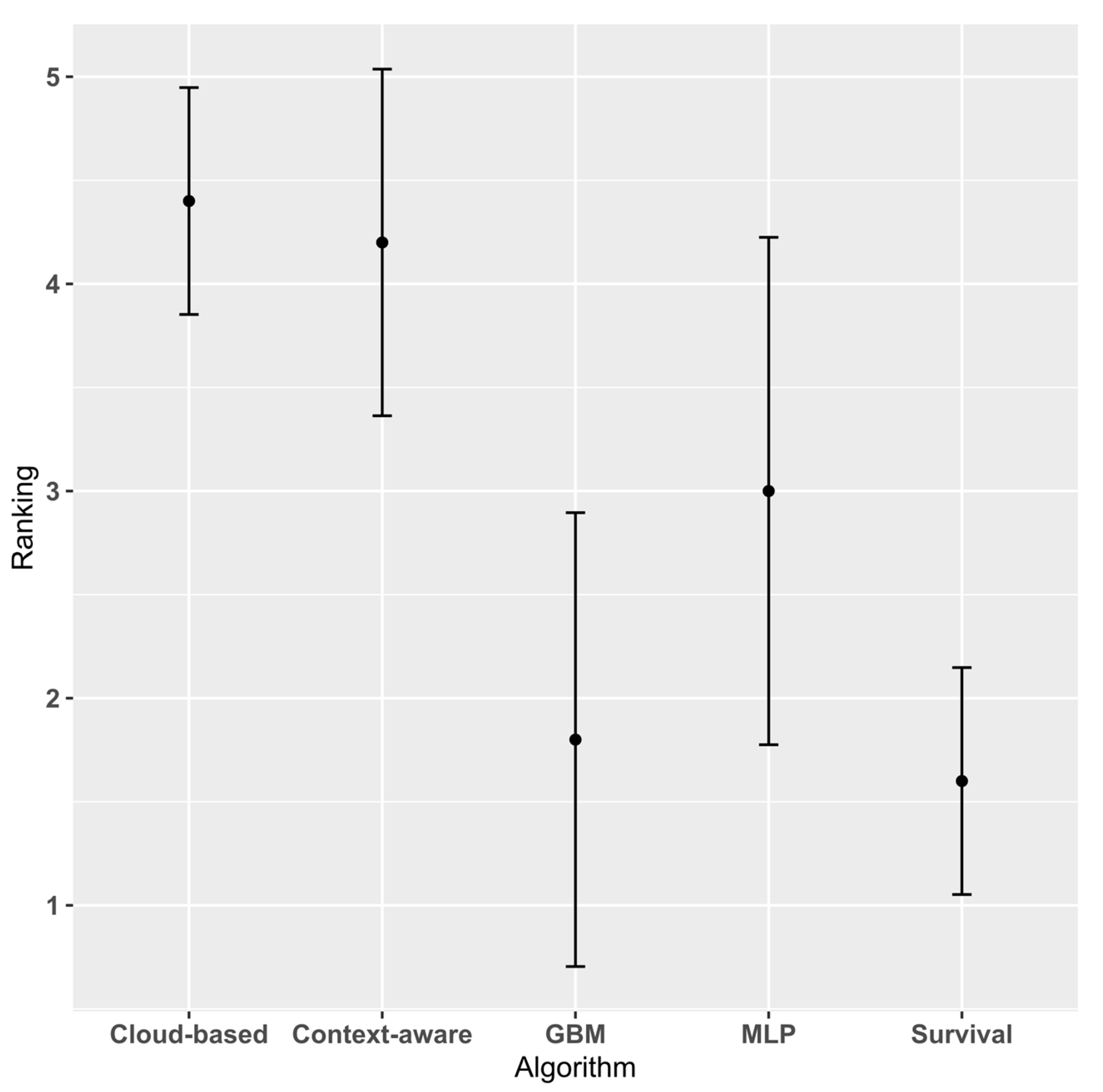
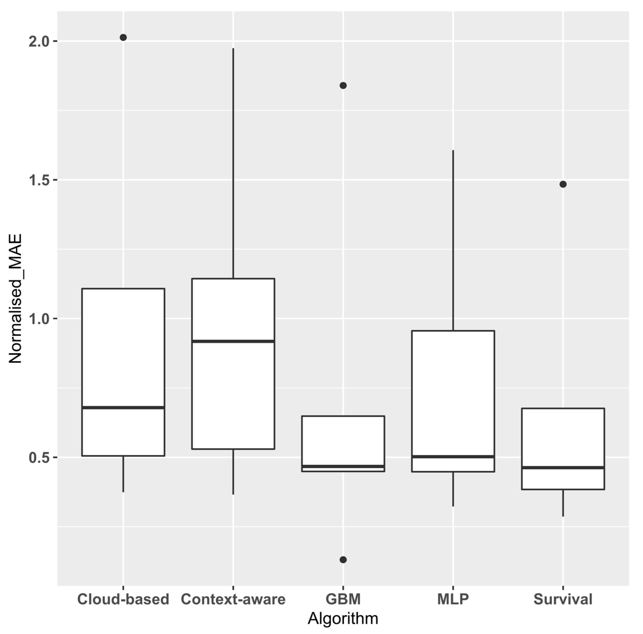
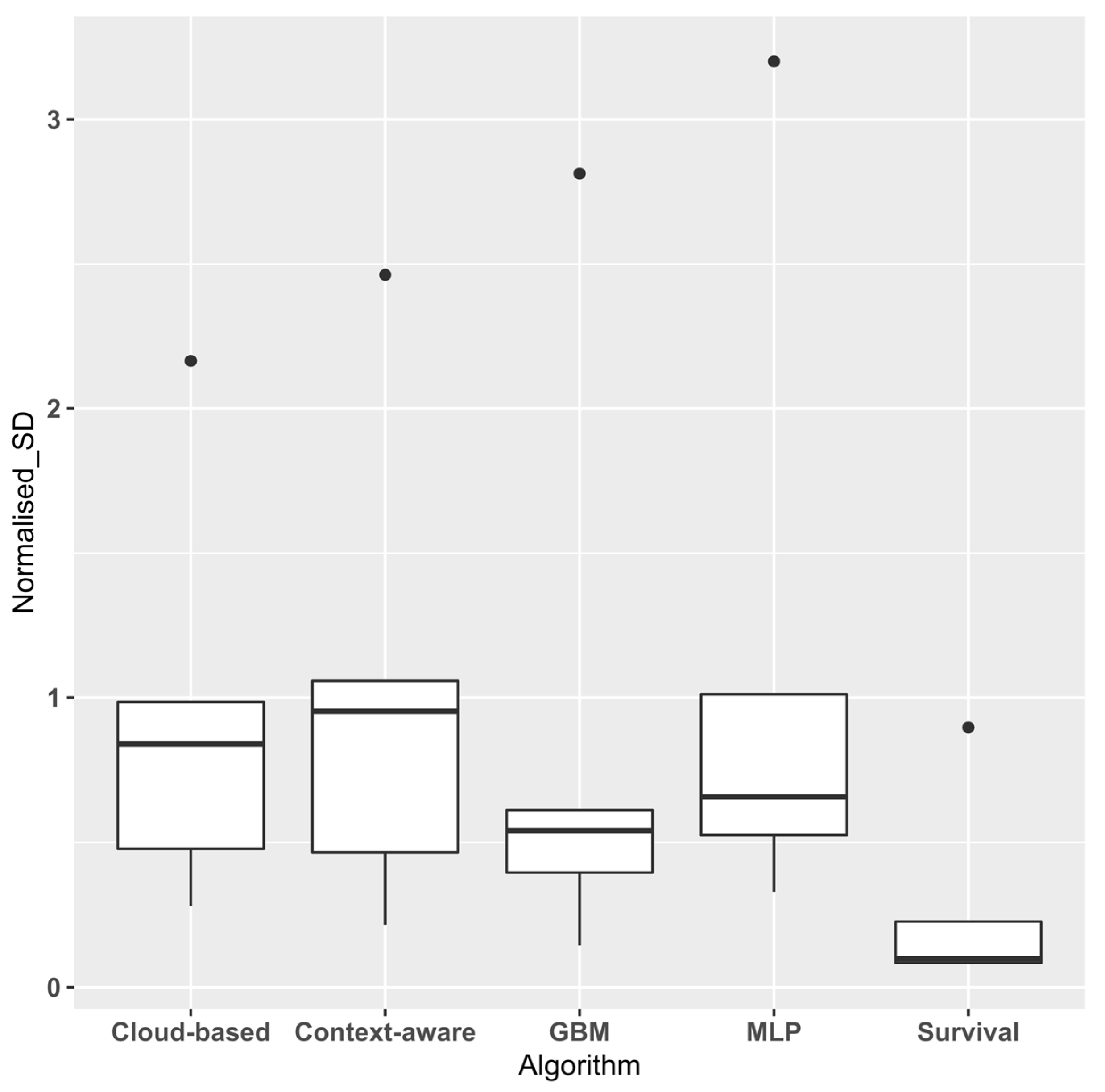
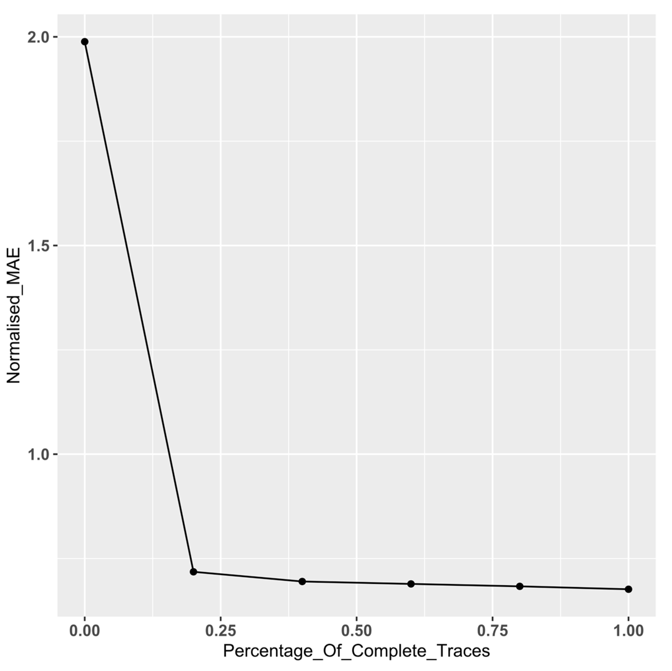
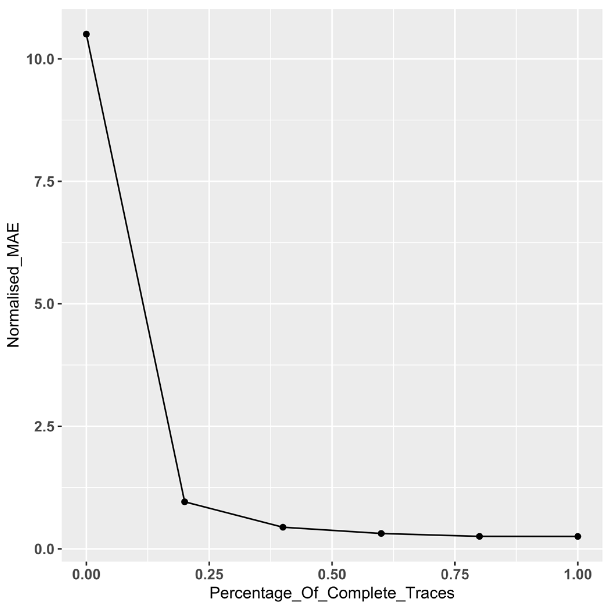
3.1. Experimental Results
3.2. Threats to Validity
4. Conclusions
Author Contributions
Funding
Conflicts of Interest
References
- Van der Aalst, W.M. Process Mining: Data Science in Action, 2nd ed.; Springer: Berlin/Heidelberg, Germany, 2016. [Google Scholar]
- Tax, N.; Verenich, I.; La Rosa, M.; Dumas, M. Predictive business process monitoring with LSTM neural networks. In Proceedings of the International Conference on Advanced Information Systems Engineering, Essen, Germany, 12–16 June 2017; pp. 477–492. [Google Scholar]
- Aslan, A. Combining Process Mining and Queueing Theory for the ICT Ticket Resolution Process at LUMC. Master’s Thesis, University of Twente, Enschede, The Netherlands, 2017. [Google Scholar]
- Rogge-Solti, A.; Weske, M. Prediction of remaining service execution time using stochastic petri nets with arbitrary firing delays. In International Conference on Service-Oriented Computing; Springer: Berlin/Heidelberg, Germany, 2013; pp. 389–403. [Google Scholar]
- Akritas, M.G. Non-parametric survival analysis. Stat. Sci. 2004, 19, 615–623. [Google Scholar] [CrossRef][Green Version]
- Somers, M.J. Modelling employee withdrawal behaviour over time: A study of turnover using survival analysis. J. Occup. Organ. Psychol. 1996, 69, 315–326. [Google Scholar] [CrossRef]
- Larivière, B.; Van den Poel, D. Investigating the role of product features in preventing customer churn, by using survival analysis and choice modeling: The case of financial services. Expert Syst. Appl. 2004, 27, 277–285. [Google Scholar] [CrossRef]
- Dirick, L.; Claeskens, G.; Baesens, B. Time to default in credit scoring using survival analysis: A benchmark study. J. Oper. Res. Soc. 2017, 68, 652–665. [Google Scholar] [CrossRef]
- Verenich, I.; Nguyen, H.; La Rosa, M.; Dumas, M. White-box prediction of process performance indicators via flow analysis. In Proceedings of the 2017 International Conference on Software and System Process Pages, ACM, Paris, France, 5–7 July 2017; pp. 85–94. [Google Scholar]
- Folino, F.; Guarascio, M.; Pontieri, L. Discovering Context-Aware Models for Predicting Business Process Performances. In On the Move to Meaningful Internet Systems, Proceedings of OTM 2012. OTM, Rome, Italy, 10–14 September 2012; Meersman, R., Panetto, H., Dillon, T., Rinderle-Ma, S., Dadam, P., Zhou, X., Pearson, S., Ferscha, A., Bergamaschi, S., Cruz, I.F., Eds.; Springer: Berlin/Heidelberg, Germany, 2012. [Google Scholar]
- Senderovich, A.; Di Francescomarino, C.; Ghidini, C.; Jorbina, K.; Maggi, F.M. ‘Intra and Inter-case Features in Predictive Process Monitoring: A Tale of Two Dimensions’. In Lecture Notes in Computer Science, Proceedings of Business Process Management. BPM 2017, Barcelona, Spain, 10–15 September 2017; Carmona, J., Engels, G., Kumar, A., Eds.; Springer: Cham, Switzerland, 2017; Volume 10445. [Google Scholar]
- Rozinat, A.; Wynn, M.T.; van der Aalst, W.M.; ter Hofstede, A.H.; Fidge, C.J. Workflow simulation for operational decision support. Data Knowl. Eng. 2009, 68, 834–850. [Google Scholar] [CrossRef]
- Veldhoen, J. The Applicability of Short-term Simulation of Business Processes for the Support of Operational Decisions. Master’s Thesis, Technische Universiteit Eindhoven, Eindhoven, The Newzerlands, March 2011. Available online: http://alexandria.tue.nl/extra2/afstversl/tm/Veldhoen%202011.pdf (accessed on 22 April 2020).
- Verenich, I.; Dumas, M.; La Rosa, M.; Maggi, F.M.; Teinemaa, I. Survey and Cross-Benchmark Comparison of Remaining Time Prediction Methods in Business Process Monitoring. Available online: https://arxiv.org/abs/1805.02896 (accessed on 11 May 2018).
- Breuker, D.; Matzner, M.; Delfmann, P.; Becker, J. Comprehensible Predictive Models for Business Processes. MIS Q. 2016, 40, 1009–1034. [Google Scholar] [CrossRef]
- Evermann, J.; Rehse, J.R.; Fettke, P. Predicting process behaviour using deep learning. Decis. Support Syst. 2017, 100, 129–140. [Google Scholar] [CrossRef]
- Pasquadibisceglie, V.; Appice, A.; Castellano, G.; Malerba, D. Using Convolutional Neural Networks for Predictive Process Analytics. In Proceedings of the 2019 International Conference on Process Mining (ICPM), Aachen, Germany, 24–26 June 2019; pp. 129–136. [Google Scholar]
- Van Der Aalst, W.M.; Reijers, H.A.; Song, M. Discovering social networks from event logs. Comput. Supported Coop. Work (CSCW) 2005, 14, 549–593. [Google Scholar] [CrossRef]
- Song, M.; Van der Aalst, W.M. Towards comprehensive support for organisational mining. Decis. Support Syst. 2008, 46, 300–317. [Google Scholar] [CrossRef]
- Nakatumba, J.; van der Aalst, W.M. Analysing resource behavior using process mining. In Proceedings of the International Conference on Business Process Management, Vienna, Austria, 1–6 September 2019; pp. 69–80. [Google Scholar]
- Everett, M.G.; Borgatti, S.P. The centrality of groups and classes. J. Math. Sociol. 1999, 23, 181–201. [Google Scholar] [CrossRef]
- Zhang, J.; Thomas, L.C. Comparisons of linear regression and survival analysis using single and mixture distributions approaches in modelling LGD. Int. J. Forecast. 2012, 28, 204–215. [Google Scholar] [CrossRef]
- Carroll, K.J. On the use and utility of the Weibull model in the analysis of survival data. Control. Clin. Trials 2003, 24, 682–701. [Google Scholar] [CrossRef]
- van Dongen, B.F. BPI Challenge 2012. 4TU. Centre for Research Data. Dataset. Available online: https://data.4tu.nl/articles/BPI_Challenge_2012/12689204 (accessed on 4 May 2020).
- van Dongen, B.F. BPI Challenge 2014. 4TU. Centre for Research Data. Dataset. Available online: https://data.4tu.nl/collections/BPI_Challenge_2014/5065469 (accessed on 4 May 2020).
- van Dongen, B.F. BPI Challenge 2015 Municipality 3. Eindhoven University of Technology. Dataset. Available online: https://data.4tu.nl/articles/dataset/BPI_Challenge_2015_Municipality_3/12718370 (accessed on 4 May 2020).
- van Dongen, B.F. BPI Challenge 2017. Eindhoven University of Technology. Dataset. Available online: https://data.4tu.nl/articles/BPI_Challenge_2017/12696884 (accessed on 4 May 2020).
- van Dongen, B.F. BPI Challenge 2018. Eindhoven University of Technology. Dataset. Available online: https://data.4tu.nl/articles/BPI_Challenge_2018/12688355 (accessed on 4 May 2020).
- van Dongen, B.F. BPI Challenge 2020. 4TU. Centre for Research Data. Dataset. 2020. Available online: https://data.4tu.nl/collections/BPI_Challenge_2020/5065541 (accessed on 26 May 2020).
- Bevacqua, A.; Carnuccio, M.; Folino, F.; Guarascio, M.; Pontieri, L. A Data-Driven Prediction Framework for Analysing and Monitoring Business Process Performances. In Lecture Notes in Business Information Processing, Proceedings of Enterprise Information Systems. ICEIS 2013, Angers, France, 4–7 July 2013; Hammoudi, S., Cordeiro, J., Maciaszek, L., Filipe, J., Eds.; Springer: Cham, Switzerland, 2014; Volume 190. [Google Scholar]
- Cesario, E.; Folino, F.; Guarascio, M.; Pontieri, L. A Cloud-Based Prediction Framework for Analyzing Business Process Performances; Springer: Cham, Switzerland, 2016. [Google Scholar]
- Ancona, D.G. Outward bound: Strategic for team survival in an organization. Acad. Manag. J. 1990, 33, 334–365. [Google Scholar] [CrossRef]
- Demšar, J. Statistical comparisons of classifiers over multiple data sets. J. Mach. Learn. Res. 2006, 7, 1–30. [Google Scholar]
- Linden, A.; Yarnold, P.R. Modeling time-to-event (survival) data using classification tree analysis. J. Eval. Clin. Pract. 2017, 23, 1299–1308. [Google Scholar] [CrossRef] [PubMed]


| BPIC 18 | BPIC 17 | BPIC 15(3) | BPIC 14 | BPIC 12 | |
|---|---|---|---|---|---|
| Number of events | 267,830 | 233,928 | 59,681 | 277,577 | 262,200 |
| Number of cases | 3285 | 9453 | 1409 | 13,985 | 13,087 |
| Number of traces | 3277 | 5211 | 1350 | 13,942 | 4366 |
| Number of distinct activities | 141 | 26 | 277 | 39 | 24 |
| Mean trace length | 81.53 | 24.75 | 42.36 | 19.85 | 20.04 |
| Mean throughput time (days) | 580.63 | 24.11 | 62.23 | 12.93 | 8.62 |
| Throughput time SD (days) | 580.62 | 14.893 | 97.64 | 27.94 | 12.13 |
| Domain | Public Admin | Financial services | Public Admin | Financial services | Financial services |
| GB | GC | GE | GD | |
|---|---|---|---|---|
| BPIC 18 | −0.058 | −0.014 | 0.248 | 0.107 |
| BPIC 17 | 0.063 | 0.176 | 0.063 | 0.093 |
| BPIC 15(3) | 0.289 | 0.414 | −0.208 | −0.045 |
| BPIC 14 | 0.078 | 0.119 | −0.183 | −0.171 |
| BPIC 12 | 0.877 | 0.848 | −0.475 | −0.003 |
| Survival | MLP | GBM | Cloud-Based | Context-Aware | |
|---|---|---|---|---|---|
| BPIC 18 | 166.27 ± 46.6 | 187.37 ± 190.62 | 76.09 ± 84.18 | 217.27 ± 162.30 | 212.34 ± 124.37 |
| BPIC 17 | 11.158 ± 2.03 | 12.11 ± 12.67 | 10.83 ± 9.54 | 12.18 ± 11.53 | 12.77 ± 11.23 |
| BPIC 15(3) | 23.91 ± 6.12 | 27.88 ± 40.91 | 29.07 ± 33.63 | 42.26 ± 52.27 | 57.12 ± 59.31 |
| BPIC 14 | 19.19 ± 11.6 | 20.78 ± 41.39 | 23.79 ± 36.37 | 26.03 ± 27.99 | 25.53 ± 31.84 |
| BPIC 12 | 5.83 ± 1.95 | 8.24 ± 8.72 | 5.59 ± 5.27 | 9.55 ± 8.49 | 9.86 ± 9.12 |
| Survival | MLP | GBM | Cloud-Based | |
|---|---|---|---|---|
| MLP | 0.04173 | |||
| GBM | 0.75592 | 0.07598 | ||
| Cloud-based | 0.00042 | 0.04173 | 0.00082 | |
| Context-aware | 0.00082 | 0.07598 | 0.00159 | 0.75592 |
| % of Complete Traces in Event Log | |||||
|---|---|---|---|---|---|
| 0% | 20% | 40% | 60% | 80% | |
| BPIC 12 | 1.2 × 10⁻⁷ | 0.0003 | 0.1158 | 0.0737 | 0.0909 |
| BPIC 18 | <2 × 10⁻¹⁶ | <2 × 10⁻¹⁶ | <2 × 10⁻¹⁶ | 2.5 × 10⁻¹⁶ | 6.0 × 10⁻¹² |
Publisher’s Note: MDPI stays neutral with regard to jurisdictional claims in published maps and institutional affiliations. |
© 2020 by the authors. Licensee MDPI, Basel, Switzerland. This article is an open access article distributed under the terms and conditions of the Creative Commons Attribution (CC BY) license (http://creativecommons.org/licenses/by/4.0/).
Share and Cite
Ogunbiyi, N.; Basukoski, A.; Chaussalet, T. Investigating Social Contextual Factors in Remaining-Time Predictive Process Monitoring—A Survival Analysis Approach. Algorithms 2020, 13, 267. https://doi.org/10.3390/a13110267
Ogunbiyi N, Basukoski A, Chaussalet T. Investigating Social Contextual Factors in Remaining-Time Predictive Process Monitoring—A Survival Analysis Approach. Algorithms. 2020; 13(11):267. https://doi.org/10.3390/a13110267
Chicago/Turabian StyleOgunbiyi, Niyi, Artie Basukoski, and Thierry Chaussalet. 2020. "Investigating Social Contextual Factors in Remaining-Time Predictive Process Monitoring—A Survival Analysis Approach" Algorithms 13, no. 11: 267. https://doi.org/10.3390/a13110267
APA StyleOgunbiyi, N., Basukoski, A., & Chaussalet, T. (2020). Investigating Social Contextual Factors in Remaining-Time Predictive Process Monitoring—A Survival Analysis Approach. Algorithms, 13(11), 267. https://doi.org/10.3390/a13110267