Before proceeding with the proof for Theorem 3, we present Lemma A1 that we will use to substantiate some intermediate claims in the theorem’s proof.
Proof of Theorem 3. We begin by noting that although other well-known arguments may be used to prove the result for some specific values of n and , but we prove all four statements using the common framework of allocation schemes and Lemma 1. Given an instance L, define to be the set of jobs accepted by Algorithm A and to be the offline optimal set. Then, the individual proofs of the four statements are as follows.
Statement 1. Given instance
L, define function
as follows:
Claim 1: is an allocation scheme from the set to the set .
Proof of Claim 1. If job , then it does not overlap with any other job in except itself (Lemma A1), and therefore, . Otherwise if job , it cannot overlap with more than 2 jobs in (Lemma A1), and therefore, . Therefore, by Definition 1, is a valid allocation scheme. □
Claim 2: for any job c in .
Proof of Claim 2. If job , then it does not overlap with any other job in except itself (Lemma A1), and therefore, . Otherwise if job , it must overlap with at least one job in because Algorithm A could not have declined job c otherwise. Therefore, . □
Since instance L was arbitrary, by Lemma 1 and Theorem 2, the result is proved. □
Statement 2. Given instance
L, define function
as follows:
Claim 3: is an allocation scheme from the set to the set .
Proof of Claim 3. If job , then it does not overlap with any other job in except itself (Lemma A1), and therefore, . Otherwise if job , the total duration of jobs in that can overlap with it is strictly less than (Lemma A1), and therefore, . Therefore, by Definition 1, is a valid allocation scheme. □
Claim 4: for any job c in .
Proof of Claim 4. If job , then it does not overlap with any other job in except itself (Lemma A1), and therefore, . Otherwise if job , it must overlap with at least one job in because Algorithm A could not have declined job c otherwise. Therefore, . □
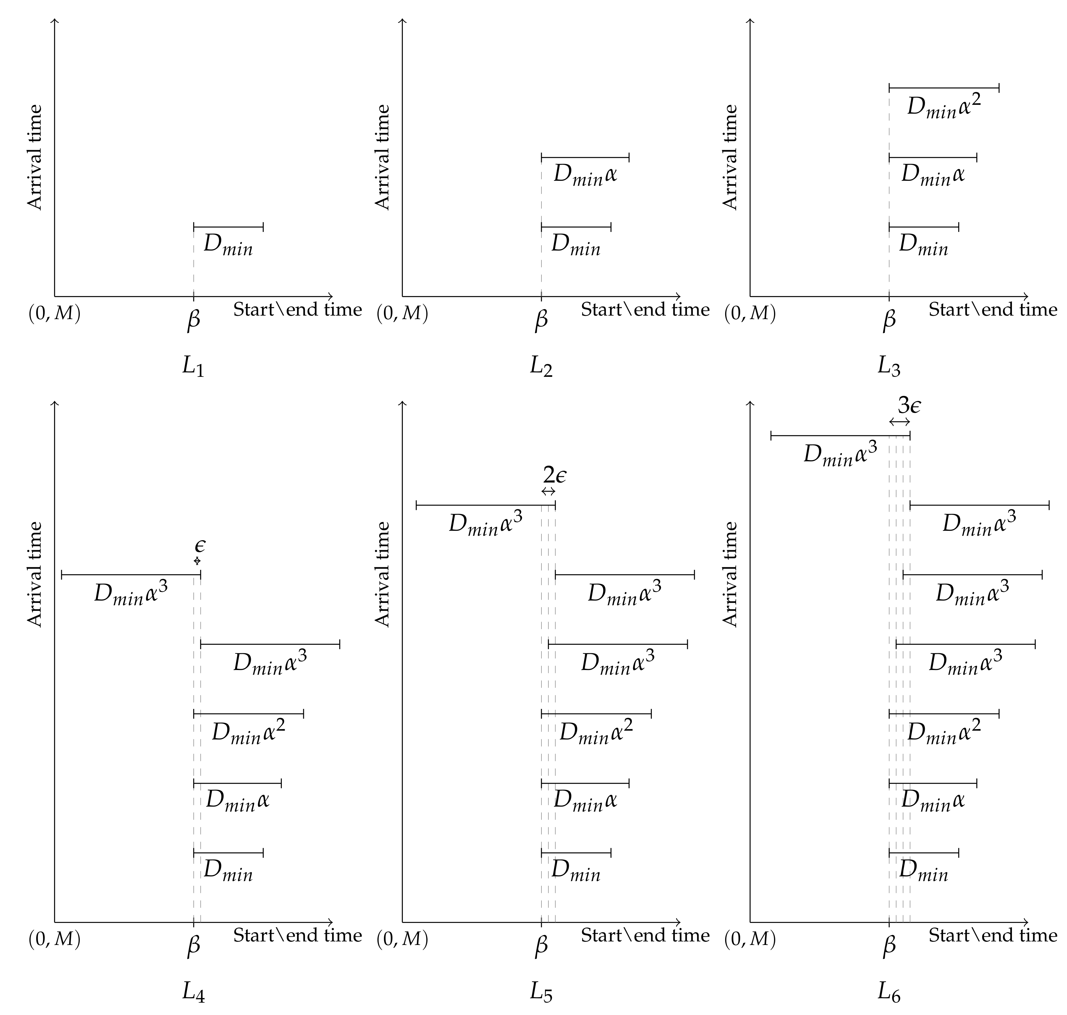
Since instance L was arbitrary, by Lemma 1, . We will now prove a matching lower bound. Let be arbitrarily large and be arbitrarily small. Consider instance L in which the jobs arrive in following sequence: . Each 2-tuple represents a job, with first value being the start time and the second being the duration. Then, . Therefore, . Since was arbitrary, this inequality holds for every , letting gives us the matching lower bound, . □
Statement 3. Given instance
L, define function
as follows:
Claim 5: is an allocation scheme from the set to the set .
Proof of Claim 5. For any job b in , at most jobs from can overlap with it (Lemma A1), and therefore, . Further, if , . Therefore, for any job , . Hence, by Definition 1, is an allocation scheme. □
Claim 6: for any job c in .
Proof□
of Claim 6. If job , then . Otherwise if job , it must overlap with at least n jobs in because Algorithm A could not have declined job c otherwise. Therefore, . □
Since instance L was arbitrary, by Lemma 1, the result is proved. □
Statement 4. Given instance
L, define function
as follows:
Claim 7: is an allocation scheme from the set to the set .
Proof□
of Claim 7. For any job
b in
, jobs from
that overlap with it have total duration strictly less than
(Lemma A1), and therefore,
Further, if , . Therefore, for any job , . Hence, by Definition 1, is an allocation scheme. □
Claim 8: for any job c in .
Proof■
of Claim 8. If job , then . Otherwise if job , it must overlap with at least n jobs in because Algorithm A could not have declined job c otherwise. Therefore, . □
Since instance L was arbitrary, by Lemma 1, . We will now prove the lower bound. Let be arbitrarily large and be arbitrarily small. Consider instance L in which the jobs arrive in following sequence:
. Each 2-tuple represents a job, with first value being the start time and the second being the duration. Then, . Therefore, . Since was arbitrary, this inequality holds for every , letting gives us the lower bound, .


