1. Introduction
The utilization of large data repositories is a crucial factor in improving various types of businesses. Such a kind of massive data repositories is defined as “big data”. Extracting the skyline objects is a vital task for understanding the dataset in the early stage of the knowledge discovery process from large data repositories. Skyline objects in a database are objects that are not dominated by any other object in the database and the skyline query [
1] is a function to find a set of skyline objects.
Given an
m-dimensional dataset
, an object
is said to be in the skyline of
if there is no other object
in
such that
is better than
. If there exists such an
, then we say that
is dominated by
, or
dominates
.
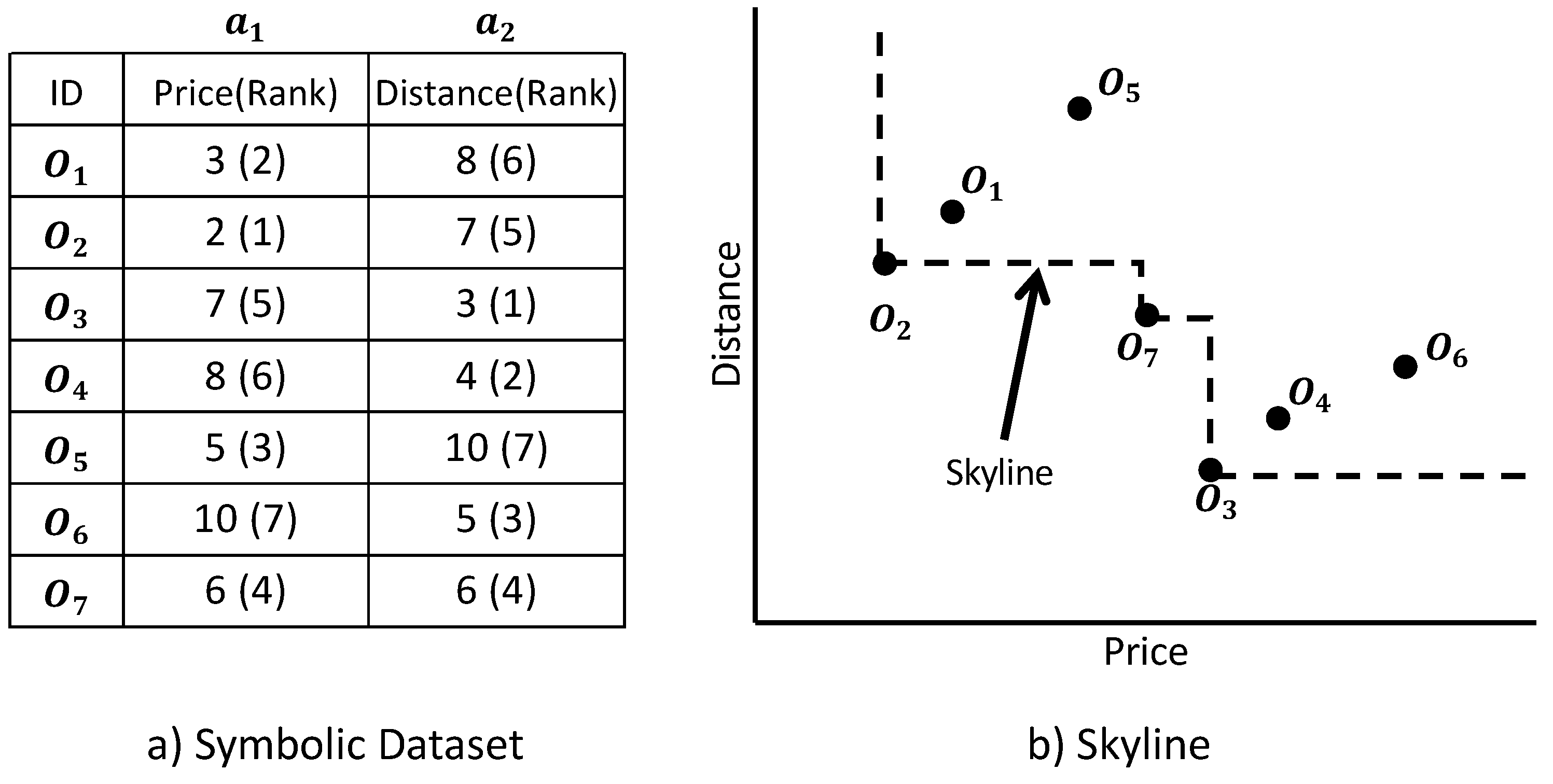
Figure 1 presents an example skyline. The table in the figure contains a list of hotels, each of which has two numerical attributes: distance and price. If we assume that a smaller value is better, then the skyline query retrieves objects
as in
Figure 1b. Objects
and
are dominated by object
. Objects
and
are dominated by object
.
Top-
k dominating query [
2] is a variant of the skyline query. In the query, a scoring function
is used for evaluating strongness of an object
:
= |{
∈
|
O≺
} |.
The scoring function
returns how many objects the object
O dominate in the dataset. In the above example,
because
dominates two objects:
and
. Similarly,
. The top-
k dominating query selects
k objects based on
. For example, a top-2 dominating query for the example in
Figure 1 retrieves
and
.
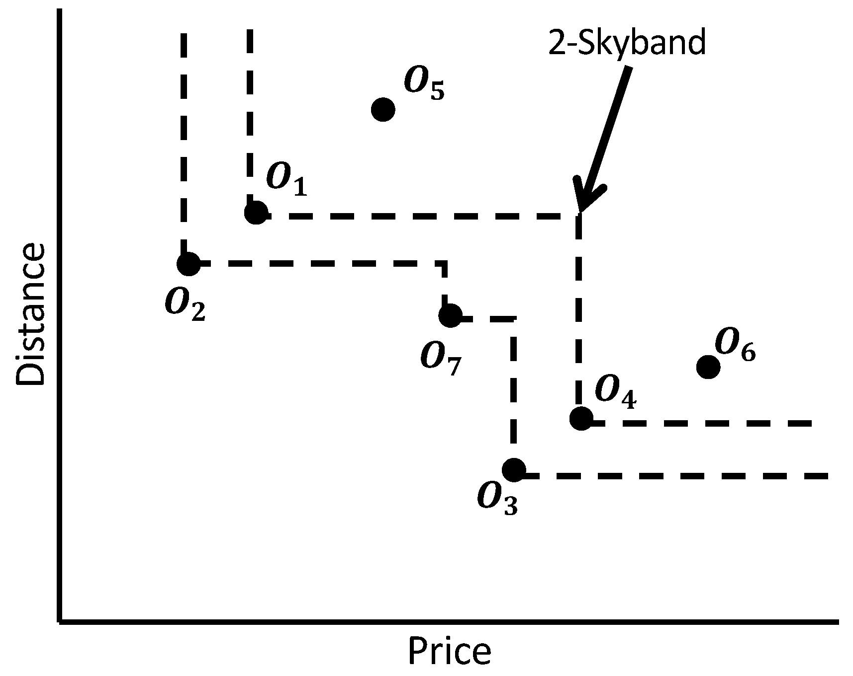
The skyband query, also known as
K-skyband query [
3], is another well known variant of the skyline query. A
K-skyband query returns a set of objects, each object of which is not dominated by
K other objects. For the dataset in
Figure 1a, the skyband query for
retrieves objects
. Object
is not in the skyband because it is dominated by two objects:
and
. Similarly, object
is not in the skyband result because it is also dominated by two objects:
and
. We illustrate this procedure in
Figure 2.
As mentioned above, recent “big data” is too large to analyze intensively. Instead of analyzing raw big data, we propose using a relatively small subset, i.e., the results of skyband and dominating queries that contain the important features of the raw data. However, conventional algorithms for computing such skyline variants are not designed for parallel distributed environments. In recent years, the MapReduce framework has been applied for parallel processing of huge amounts of data on large-size clusters of commodity computers in a reliable manner. MapReduce and Hadoop, which is a popular open source variant of MapReduce, has attracted significant research attention. Our parallel algorithm utilizes the MapReduce framework. In this paper, we propose a MapReduce algorithm, i.e., a parallel algorithm that simultaneously computes skyband and dominating query.
The contributions of this paper can be summarized as follows:
We examine the skyband and dominating queries for processing “big data”.
We develop a scalable parallel algorithm to compute the queries. The proposed algorithm simultaneously computes skyband and dominating queries. Exploiting the MapReduce framework for the skyband as well as dominating queries is an innovative approach that utilizes the advantage of parallel distributed computing environment.
The main focus of the proposed algorithm is to distribute the computation process evenly among multiple computing nodes so that “big data” can be effectively processed. We empirically prove the efficiency of the proposed method through intensive experiments using a real dataset and synthetic datasets.
The organization of this paper is as follows. We survey the literature and review related works in
Section 2. We present the concepts and properties of skyband and dominating query in
Section 3. We describe analysis of proposed algorithm with detailed examples in
Section 4. Next, we evaluate our algorithm through intensive experiments in
Section 5. Finally, in
Section 6, we conclude this paper.
2. Related Works
Skyline query and its variants have been widely used in several multi-criteria decision support applications. Borzsonyi et al., who first introduced the skyline query, proposed three basic algorithms for the skyline computation [
1]. Those algorithms are known as block-nested-loops (BNL), divide-and-conquer (D&C), and B-tree-based schemes. Chomicki et al. proposed a sort–filter–skyline (SFS) algorithm, which improved the efficiency of the skyline computation by presorting the database attributes [
4]. To optimize the average-case running time, Godfrey et al. proposed linear elimination sort for skyline (LESS) algorithm [
5]. To filter the dominated objects efficiently through recursively partitioning the dataset based on the nearest objects, Kossmann proposed the nearest neighbor (NN) algorithm for computing the skyline [
6].
On the other hand, instead of computing skyline from the original objects’ attributes, several algorithms have proposed to use the index of the objects’ attributes for computing skyline. Tan et al. has proposed two progressive algorithms to compute skyline based on attributes’ bitmap and index [
7]. The recent state-of-the-art algorithm is the
-
-
, proposed by Papadias et al., which is shown to be I/O optimal for computing skylines on datasets indexed by R-trees [
3]. Meanwhile, various approaches have been proposed for effective skyline querying from the high dimensional dataset. Yuan et al. proposed a
structure to reduce the cost of skyline computation over all possible subspaces [
8]. Later, Xia et al. revised the
structure and proposed CSC structure as a more promising alternative for removing identical skyline objects in the
by storing each skyline object only to its minimum-subspace [
9].
As a variant of the skyline query, Chan et al. introduced the concept of top-
k frequent skyline queries [
10]. They suggested that a metric, called
skyline frequency, can be used to rank and select skyline objects by their interesting-ness. Li et al. proposed a data-cube structure to speed up the query evaluation by analyzing the dominance relationship [
11]. On the other hand, Lin et al. have considered extracting k most representative skyline objects [
12]. They have introduced the concept of a representative object by the population it dominates. According to their definition, a skyline object is more representative than other skyline objects, when it dominates more objects than others. Chan et al. illustrated
k-dominant skyline based on the measure of the
k-dominance relationship. The
k-dominant skyline query can control the number of retrieved objects by changing
k. If we set a larger
k value, an object more likely to be dominated by another object. They developed specialized algorithms to compute the
k-dominant skyline [
13].
K-skyband query, which is another variant of skyline query, selects those objects which are dominated by at most (
K-1) other objects. It has been noticed that, for any increasingly monotone aggregate function, the top-
k objects belong to the k-skyband, where
[
3,
14].
There exist more spontaneous techniques for skyline query formalization. Lin et al. proposed
n-of-
N skyline query to support online query on data streams, i.e., to find the skyline of the set composed from the most recent
n elements. The proposed method considers a very widely distributed dataset, which is impossible to process in a centralized fashion [
15]. Balke et al. has also investigated skyline computation over a vertically distributed database [
16]. Tao et al. examined skyline query in arbitrary subspaces [
17]. Papadias et al. studied on dynamic skyline query [
18]. Dellis et al. proposed the reverse skyline query, which selects the number of users who like the given object most based on the dominance relationship among the objects [
19].
Nowadays, the parallel computing paradigm becomes very popular for processing and analyzing “big data”. Therefore the computation of skyline and its variants are becoming challenging today. Noted that [
10,
11,
13] cannot be directly applied to evaluate top-
k dominating queries. Moreover, the computation of skyband query requires a separate algorithm. This paper proposed an efficient algorithm for computing both types of queries(top-
k dominating and skyband) over a large volume of data, such as “big data”. For such data intensive applications, the most notable platform, which has attracted a lot of attention, is MapReduce For this kind of data-intensive application, the MapReduce framework has attracted much attention as the most prominent platform [
20,
21,
22]. It facilitates the deployment of scalable parallel applications on the share-noting machines cluster for processing large dataset. Google’s MapReduce or its open source equivalent Hadoop is a powerful tool for building such applications [
23]. The MapReduce framework has also been utilized for some of the recent research works on the computation of skyline and
k-dominant skyline [
24,
25,
26].
Recently, Ezatpoor et al. [
27] exploits the MapReduce framework for computing top-
k dominance on incomplete big data. Besides, Chen et al. [
28] utilized the Spark streaming framework to process top-
k dominating query over the distributed data stream. Both [
27,
28] divided the data by using the method of the hash map to process the data through distributed computing nodes.
This paper complements the existing efforts to address the K-skyband and top-k dominating query problems by the rank of objects obtained using two intuitive scoring functions. Specifically, our algorithm can provide solutions for these two types of queries within the same framework. To the best of our knowledge, there is no such MapReduce algorithm had been proposed for the k-dominating query and the K-skyband query so far.
3. Preliminaries
Consider an
m-dimensional dataset
. We assume that the dataset is distributed into
n subsets
in different locations. Without loss of generality, we assume that the dataset contains non-negative numerical values. We also assume that smaller values are preferable in each dimension/attribute.
.
denotes that the
p-th dimension’s/attribute’s value for object
, where
is an object
which means object
j in dataset
i (
). Assume that the dataset
shown in
Figure 1 is distributed into three subsets,
, and
, each of which has two attributes,
and
, as shown in
Table 1.
Definition 1. (Dominance) For two objects O and , object O is said to dominate object , denoted , if for all attributes () and for at least one attribute (). We refer to such an O as a dominant object and such a as A dominated object. If O dominates , then O is preferable to .
In
Table 1, object
dominates object
(
). This is because object
has a smaller value for both attributes than object
.
Definition 2. (Skyline) An object is in a skyline of (i.e., a skyline object in ) if O is not dominated by any other object in . The skyline of , denoted , is the set of skyline objects in . For the dataset , objects , and can dominate all other objects and are not dominated by any other object. Therefore, a skyline query on dataset will retrieve = , .
Definition 3. (The μ score) The μ score of an object shows how many objects the object dominate in the dataset. We use to denote the μ score of an object O. In Table 1, object dominates objects and . Therefore, the μ score of is 2 (i.e., ). Definition 4. (The score). The score of an object is the number of objects dominating that object. We use to denote the score of an object O. In Table 1, object is dominated by objects and . Therefore, the score of is 2 (i.e., ). Definition 5. (Dominating query) Given a positive integer k and a dataset , the top-k dominating query returns the k objects that have the top-k μ scores in . For the dataset in Table 1, a top-two dominating query retrieves and . Definition 6. (Skyband query) Given a positive integer K, the K-skyband is the set of objects that are not dominated by K other objects. For the dataset in Table 1, the skyband query for retrieves objects . Intuitively, K represents the thickness of the skyline. A 1-skyband query is the same as a conventional skyline query. Definition 7. (Worst rank) For an object O, assume and are the rank values of attributes and , respectively. For example, in Figure 1, and . We refer to the largest () as “the worst rank of O” and as “the worst rank attribute of O.” In this example, the worst rank of was six and the worst rank attribute was . Definition 8. (Domination check set) The domination check set () for an object O is the set of objects that have equal or greater rank than the worst rank of O for the worst rank attribute. For example, has a greater rank than the worst rank of (7th > 6th) in (price). Therefore, the set of object is . Similarly, the worst rank of is 6 in (distance). So, the set of object is .
From the above definitions, we have observed an important property [
28] and a lemma.
Property 1. Top-k dominating queries result always comes from skyband queries result. For example, a top-two dominating query for the example in Figure 1 retrieves and . Those are also belongs to two-skyband result (Figure 2). Lemma 1. Dominance relation among the objects within a dataset also remains in the transformed ranked dataset. For example, in Figure 1 object dominates object , since object has a smaller value for both attributes than object . This dominance relation is also true according to the rank dataset. This is because object has a greater rank for both attributes than object . 4. Skyband and Dominating Query Processing
Our MapReduce-based algorithm for skyband and dominating queries consists of the following five phases:
P1: Data map and ranking. Each distributed dataset was partitioned vertically. Then, each partition was dispatched to the map workers (mappers). Each map worker, next, generates (, ) pairs, where is the numeric value of the corresponding object in the attribute domain and represents the object . After receiving (, ) pairs as input, each “reduce” worker (reducer) produced the (, ) pairs for each object, where is the rank value of each object in the attribute domain.
P2: Shuffling. In this phase, each map worker outputs (, ) pairs, where is the attribute name with the corresponding attribute rank for each object in the attribute domain. Next, each “reduce” worker also produced (, ) pairs for each object, where is a list of attribute names and the respective rank value for each attribute.
P3: Worst rank computation. The coordinator collected all pairs to reduce data transmissions from map workers to reduce workers. After rearranging the pairs, the coordinator found the worst attribute rank for each object.
P4: DC sets computation. The coordinator sends the attributes with the worst ranks to the workers, which are responsible for set computation for each object. Each worker takes an attribute rank, and the corresponding attribute’s worst rank as input and outputs sets for each object.
P5: Skyband and dominating objects computation. At this stage, the map workers take sets as inputs and perform domination checks between the sets and corresponding objects. Finally, the reducer produced the score and the score required to compute the skyband query and top-k dominating query, respectively.
4.1. Data Map and Ranking
We first vertically split the dataset into m partitions, if the number of attributes in a dataset is m. Therefore, if the number of data subsets was n, then the total number of partitions was equal to (e.g., ). For simplicity, we denote , , and as , , ⋯, and , respectively. In the example, had two attributes and . We split into two partitions called and . Since we had two partitions, we needed at least two map workers to complete the computation.
Figure 3 illustrates the “data map and ranking” procedure. Figure shows that objects
and
have rank “1" for attribute
and
, respectively. Therefore,
had the smallest
value and
has the smallest
value.
Recall that in the Hadoop framework in which we have implemented our system, each map worker operates on a non-overlapping partition of the input file independently and the worker emits key-value pair lists in parallel according to a user-defined “map function”. In proposed algorithm, each map worker produces (, ) pairs, where is the numeric value of each object in the attribute domain and is the corresponding object . Next, the reduce workers begin their processing job. They receive (, ) pairs as inputs and produce (, ) pairs for each object, where is the ascending order sorted rank value of each object in the attribute domain. To calculate the rank value for each key-value pair of , the corresponding reduce worker sorts its attribute in ascending order. The reduce worker, then, replaces the values with their corresponding ascending rank value.
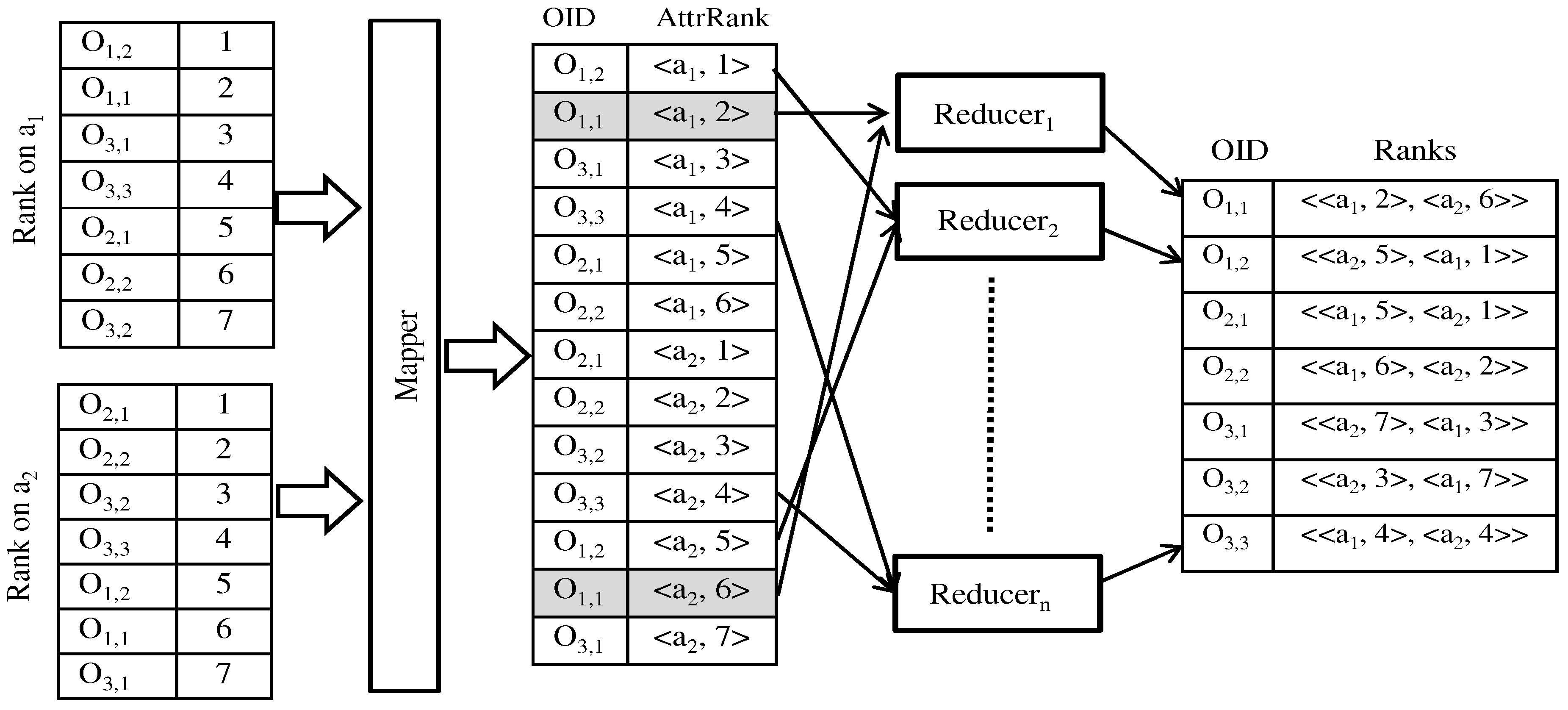
4.2. Shuffling
The second MapReduce phase is invoked for skyband and top-
k dominating query computation. After generating
pairs in the data map and ranking phase, map workers take those pairs as inputs and produce (
,
) pairs, where
is the attribute name with the corresponding attribute rank for each object in the attribute domain. Then, each map worker dispatches the (
,
) pairs to the reducers. After shuffling, reduce workers produce (
,
) pairs for each object, where
is a list of attribute names and respective rank values for each attribute.
Figure 4 illustrates the “shuffling” procedure. In the example,
has rank values of two and six for attributes
and
, respectively. Therefore, map workers produce two key-value pairs,
and
, for
. After shuffling those two pairs, the reduce worker generates an
pair for object
as a key-value pair, which is (
). Each reduce worker dispatches
pairs to the coordinator.
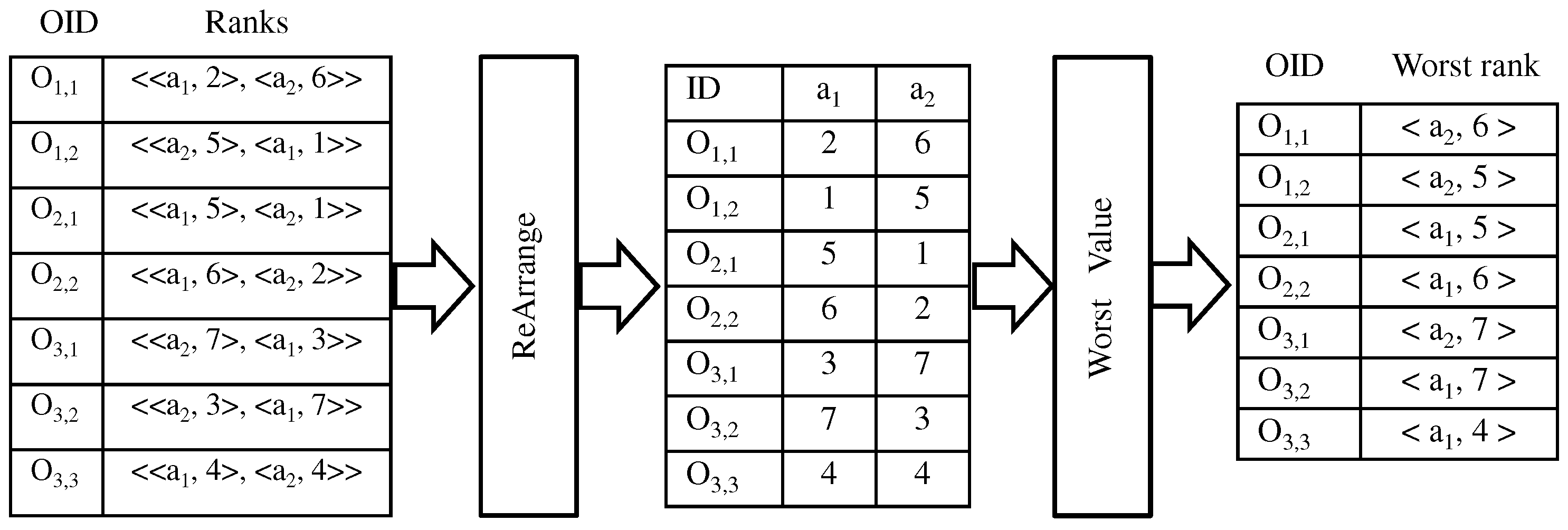
4.3. Worst Rank Computation
The coordinator computes the worst rank and corresponding worst rank attribute for each object.
Figure 5 illustrates the “worst rank computation” by the coordinator. In the example,
has rank values of two and six for attributes
and
, respectively. In the object,
’s rank is the worst among all attribute ranks. Therefore, the worst rank of
is six and the corresponding worst rank attribute of
is
. Therefore, the coordinator generates (
) as a key-value pair for
.
4.4. DC Sets Computation
The coordinator distributes the output pairs to the workers according to the worst rank attribute.
Figure 6 presents the “
sets computation” procedure. As shown in the figure, pairs of
,
,
, and
are distributed to worker
for
. Similarly, pairs of
,
, and
are distributed to worker
for
.
Each worker outputs
sets for each object. In
Figure 6, because object
has the worst rank of 5 in
,
outputs
as the
set for
. It should be noted that
and
have a greater rank than that of
in
. Object
has the worst rank of 6 in
and
outputs the
set member of
as
. We calculate the
sets for other objects similarly.
4.5. Skyband and Dominating Objects Computation
Each map worker takes the previous sets as inputs and performs domination checks between corresponding objects and sets to produce pairs, where the score is the number of objects dominated by an object. In contrast, the score of an object is the number of dominant objects. However, to compute either a score or score, our method does not need to perform a domination check with any objects outside the sets. This advantage stems from the following theorem.
Theorem 1. For two objects , if is not in the set of object O, then O cannot dominate object (i.e., ).
Proof. Let be the worst rank attribute of O. If O dominates , must be in the set of O because . If is not in the set of O, it means . Therefore, O cannot dominate . □
Theorem 1 demonstrates that it is sufficient to perform a domination check between an object O and the corresponding set to determine whether or not O is in the query results. To analyze this result, recall object and its corresponding set . Because has the worst rank of 5 for attribute , this means that this object has no possibility to dominate a higher rank object, such as , or . This means we need to perform a domination check only between and its set .
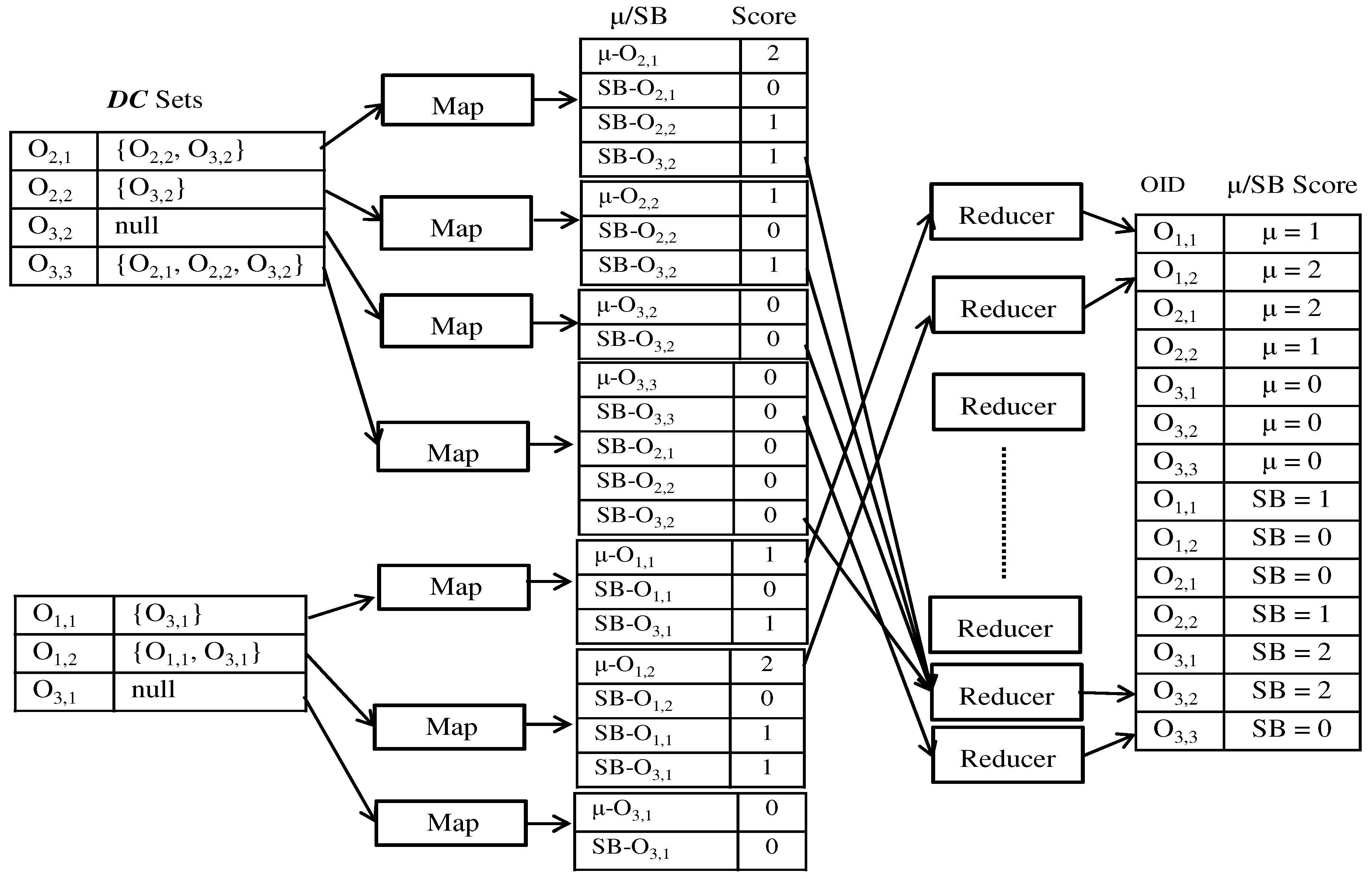
Figure 7 presents the skyband and dominating objects computation process. To compute
K-skyband, if we set
, the query returns
,
,
,
,
as the two-skyband objects set, since the
score values for these objects is less than 2. Then, our method outputs objects
and
as the top-2 dominating result because both objects have the highest
score value.
After performing a domination check, each map worker produces two types of keys: the score for the corresponding object and the score for all objects. If an object dominates another object in the set, the score value of the corresponding object and score value of the dominated objects are incremented by 1. Next, all of the scores and scores are sent to the reduce workers. After applying a “group-by” operation, the reduce workers can provide K-skyband and top-k dominating query results.


