Hybrid MU-MIMO Precoding Based on K-Means User Clustering


Abstract
:1. Introduction
2. Precoding Schemes
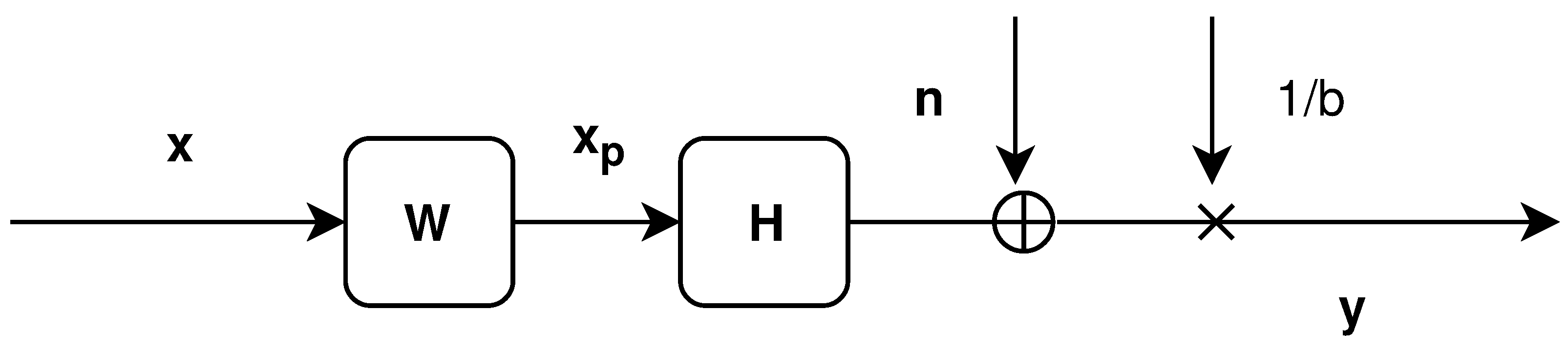
2.1. Linear Precoding
2.2. Non-Linear Precoding Schemes
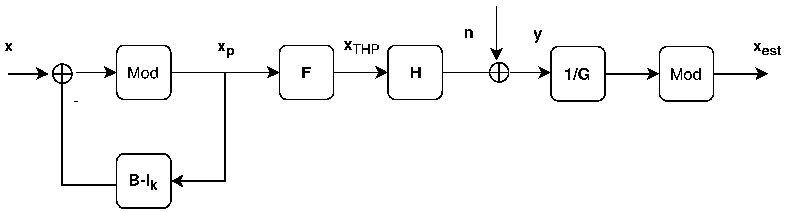
2.2.1. THP Precoding
2.2.2. Vector Perturbation Precoding
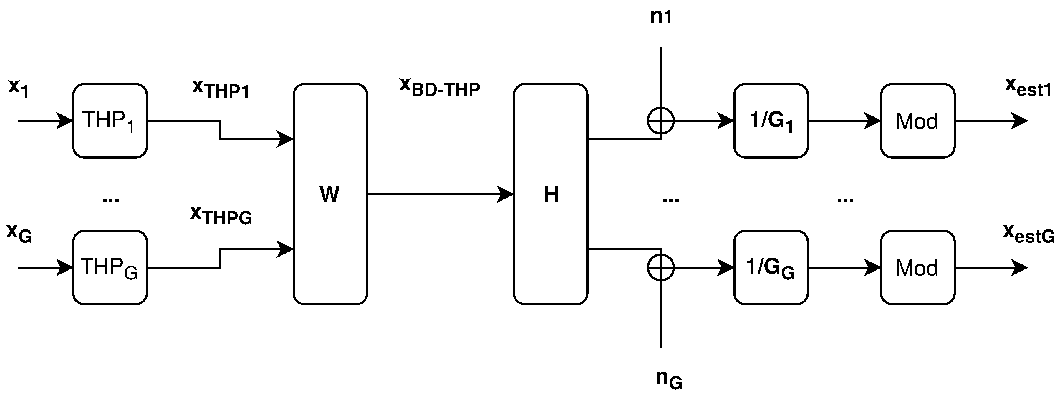
2.3. Hybrid Precoding
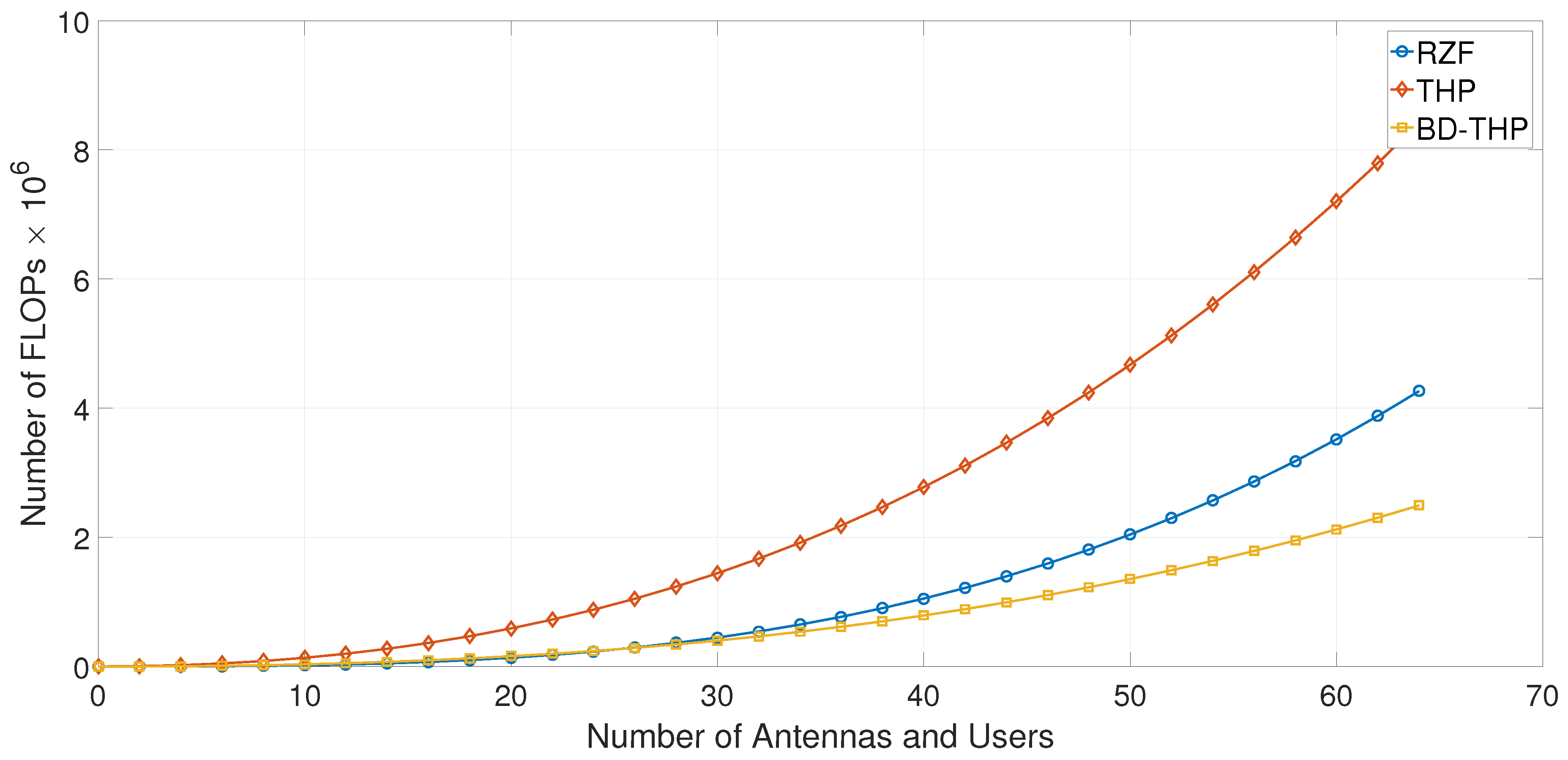
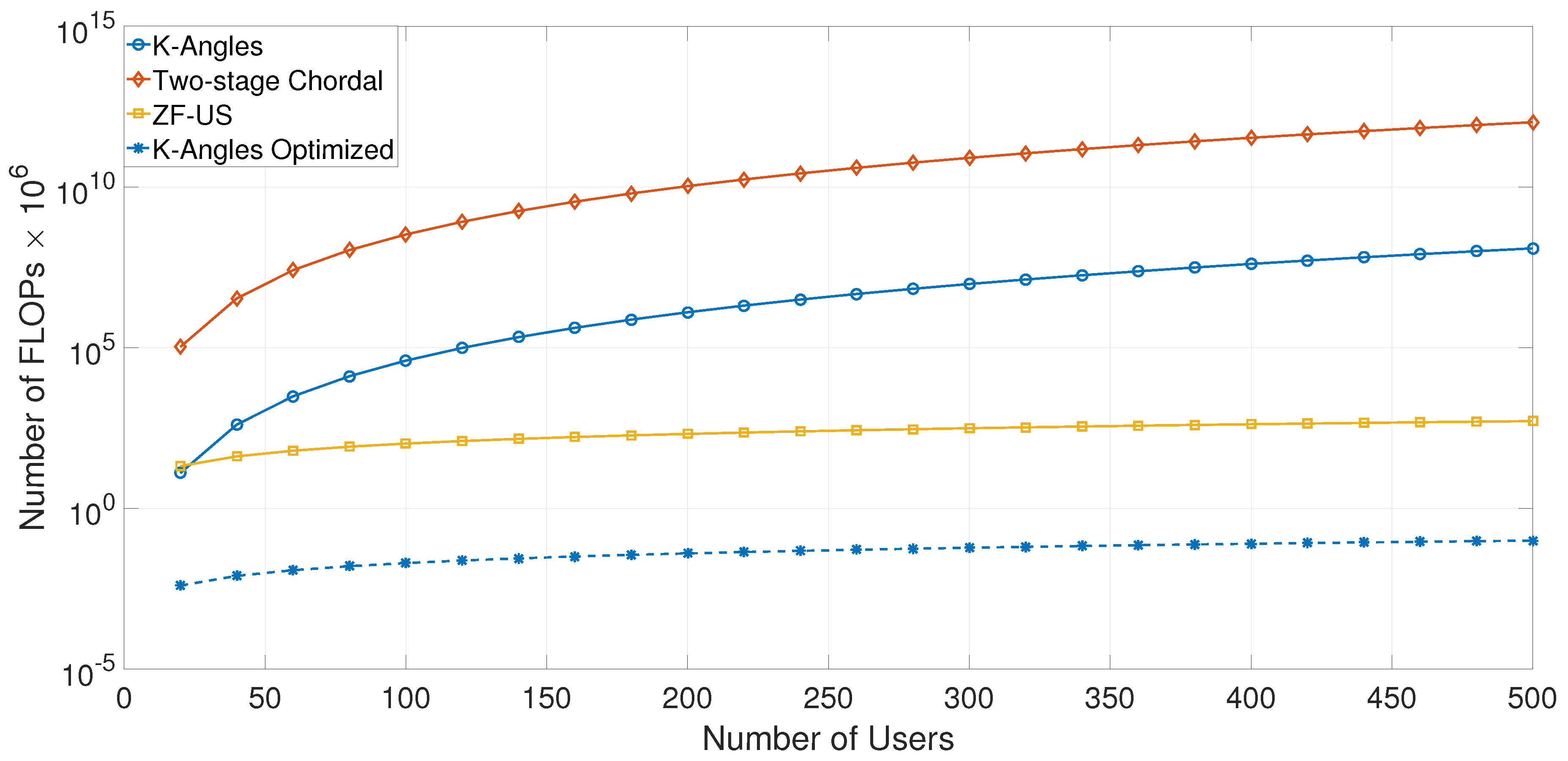
2.4. Complexity Evaluation
3. Spatial Compatibility and Channel Modeling
3.1. Channels Separation Metric
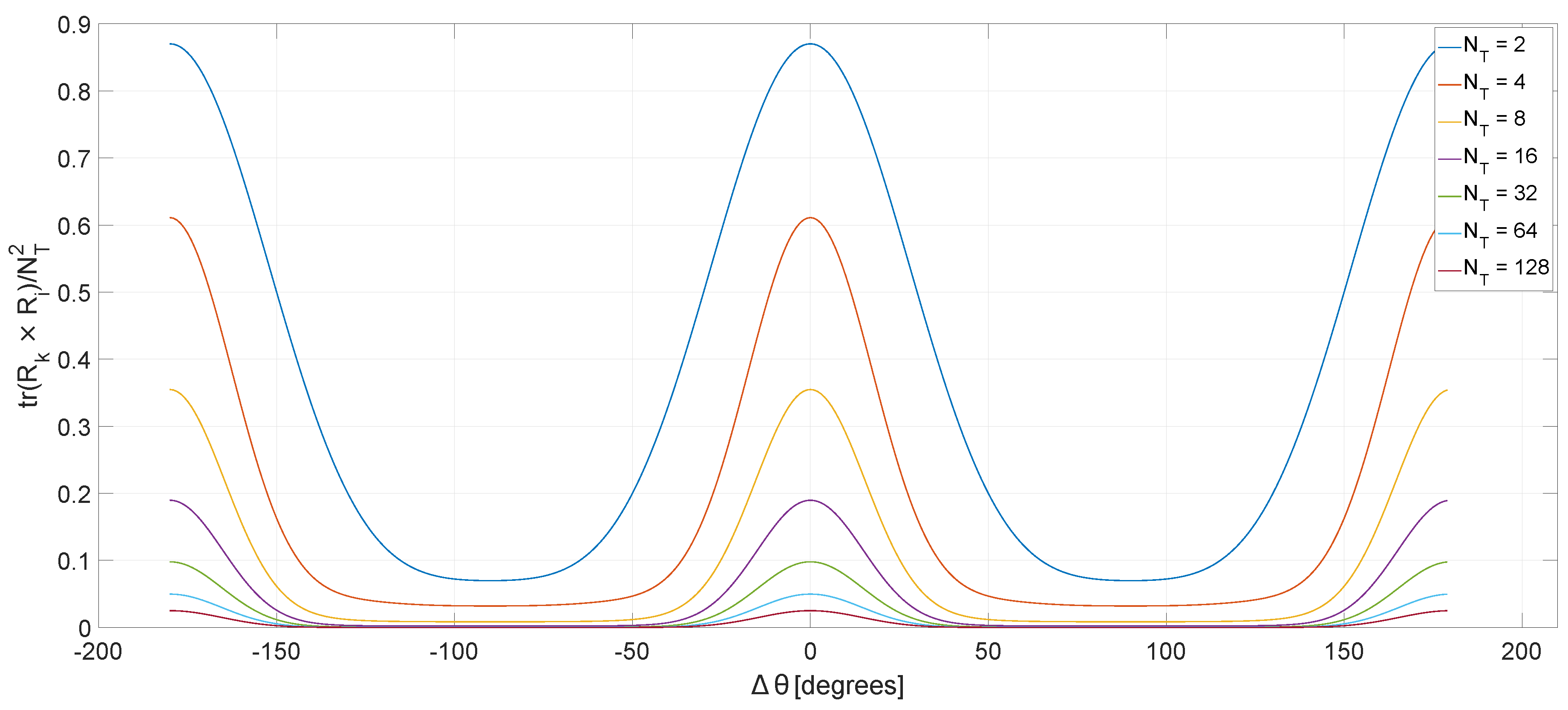
3.2. Correlation Model
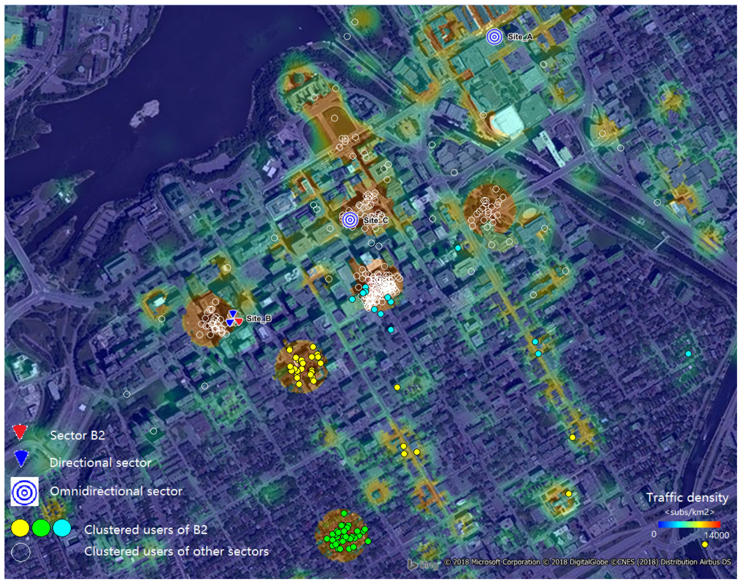
4. User Grouping
| Algorithm 1 K-means clustering. |
|
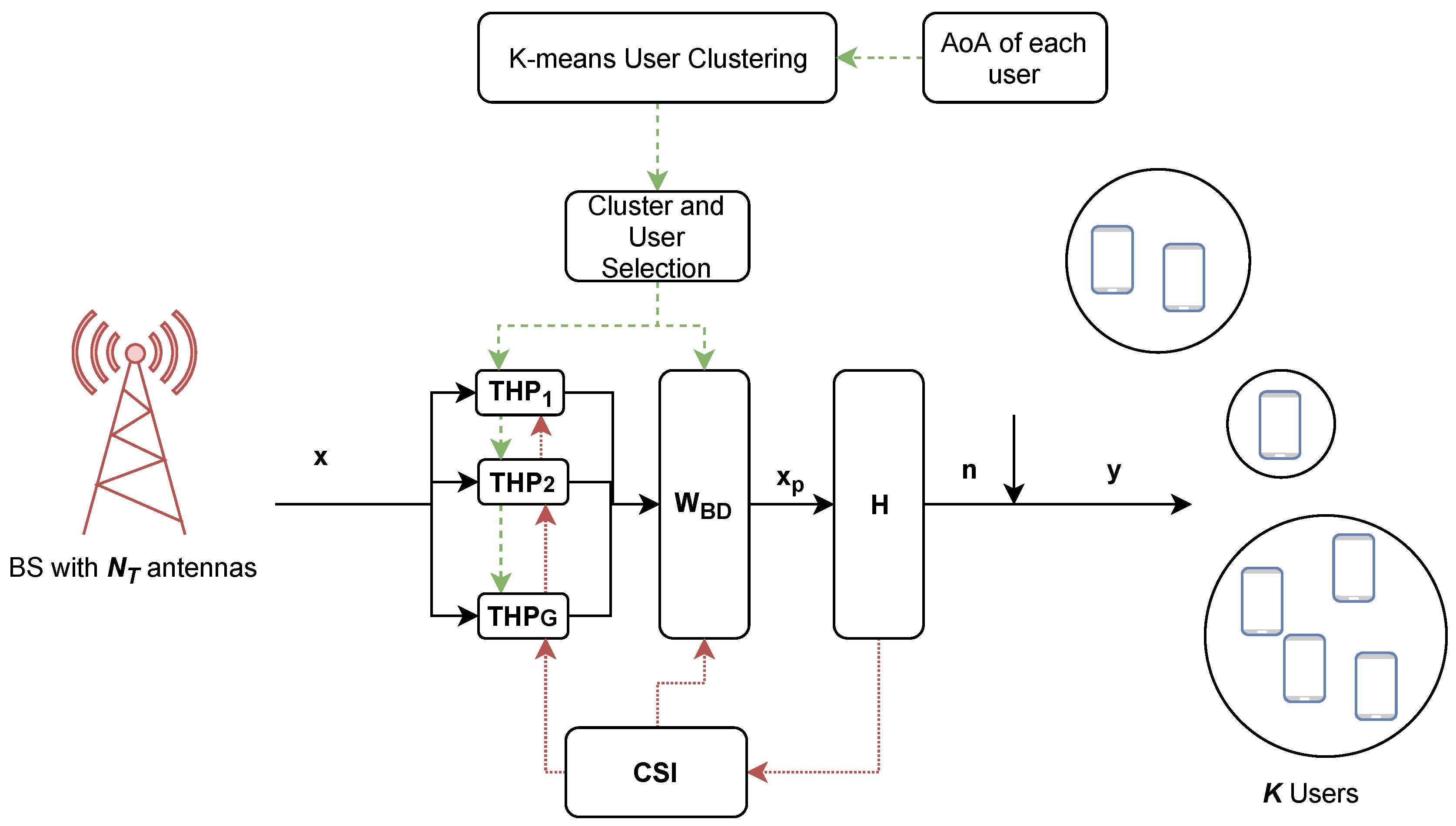
5. System Model
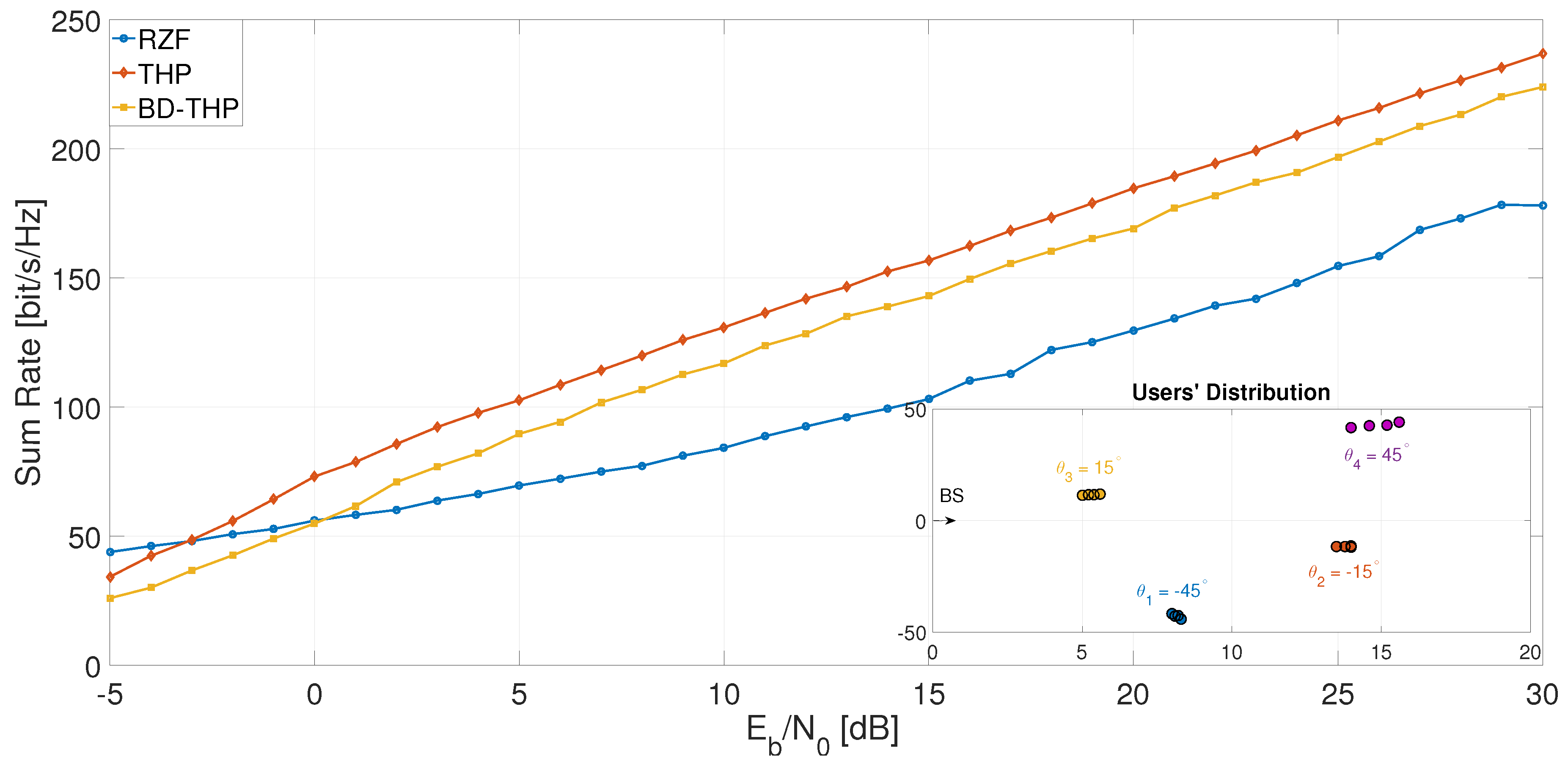
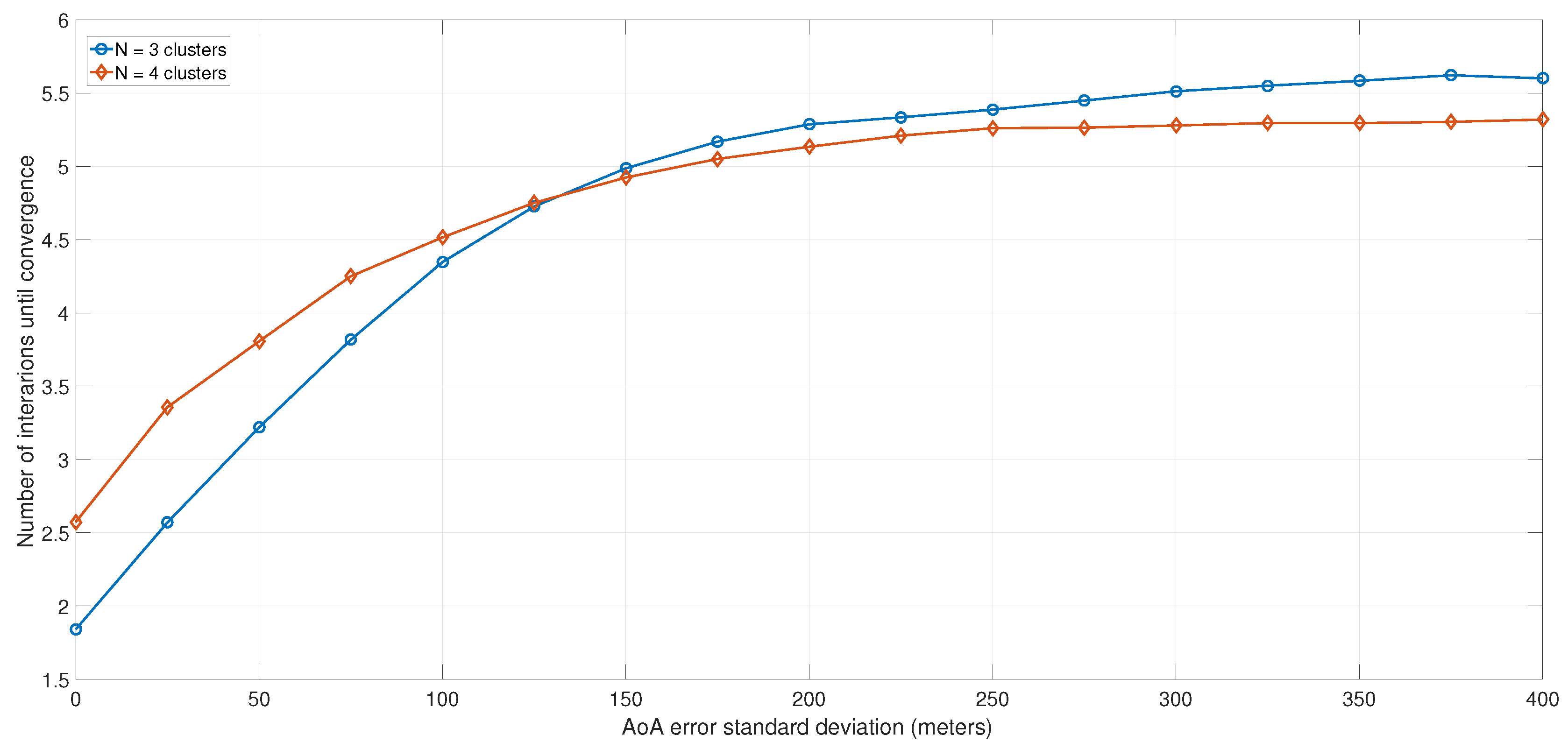
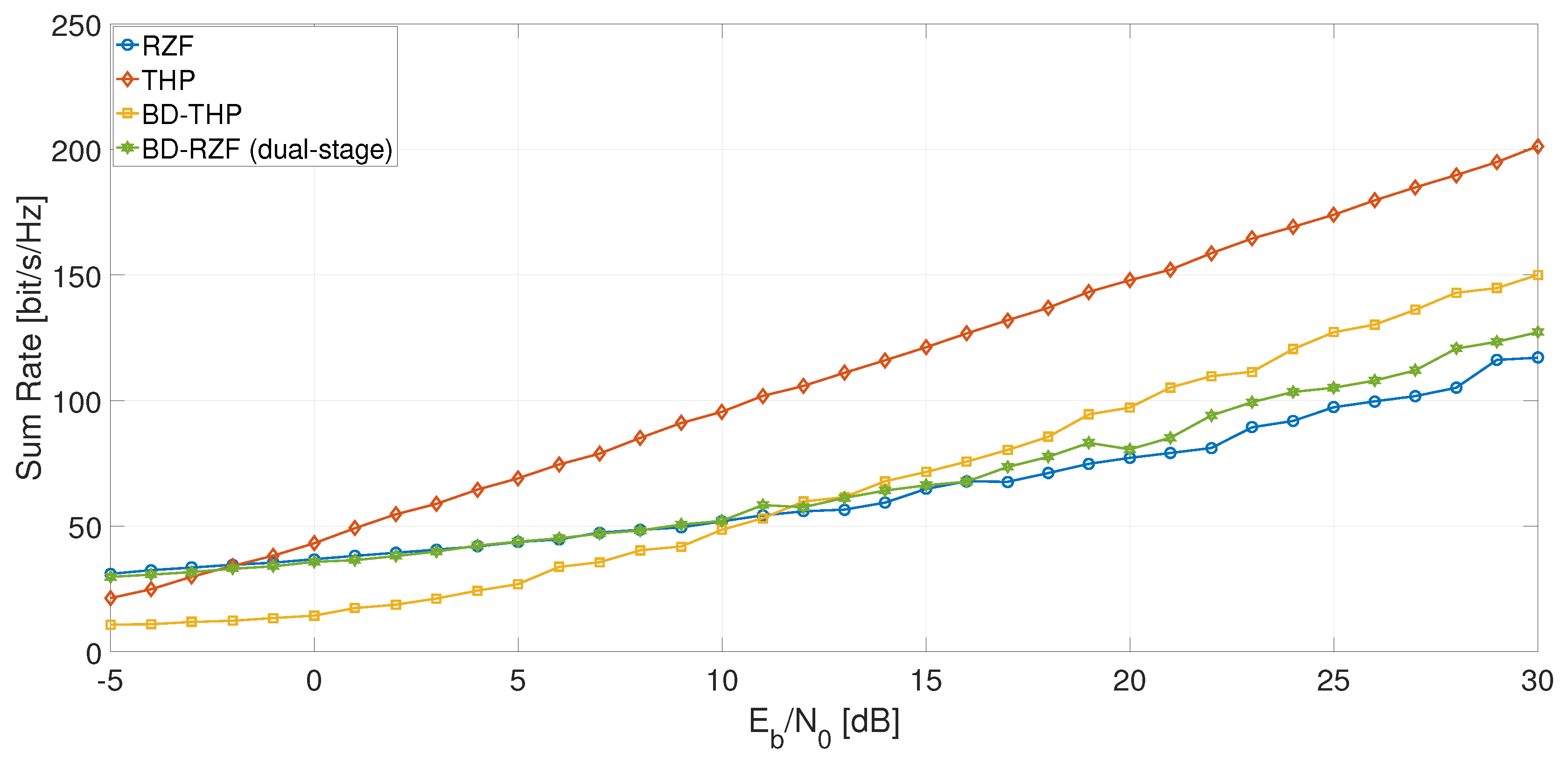
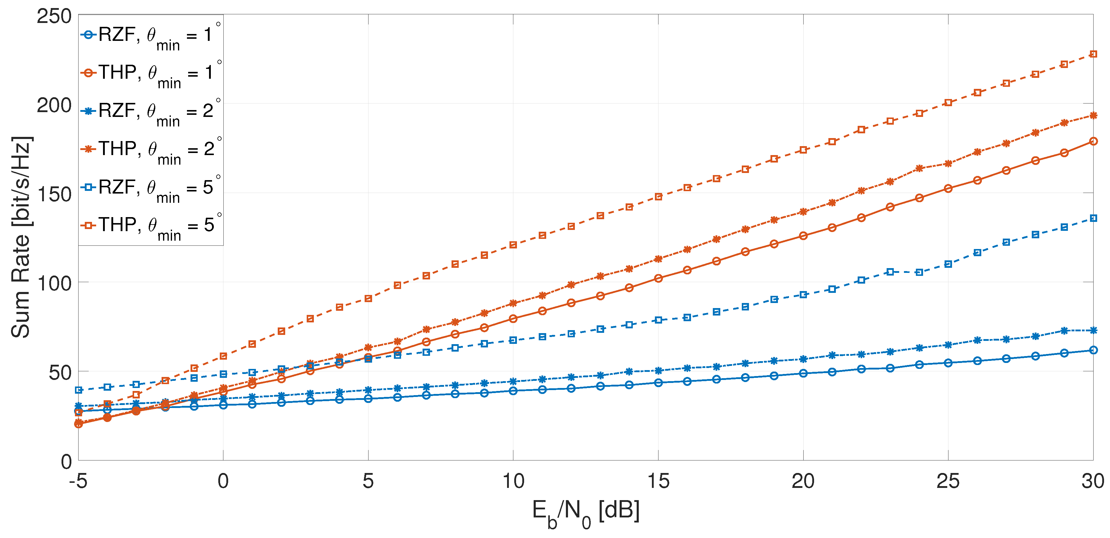
6. Simulations
7. Conclusions
Author Contributions
Funding
Conflicts of Interest
References
- Chien, T.V.; Bjornson, E. Massive MIMO Communications, 5G Mobile Communications; Springer: Basel, Switzerland, 2017; pp. 77–116. [Google Scholar]
- Castaneda, E.; Silva, A.; Gameiro, A.; Kountouris, M. An Overview on Resource Allocation Techniques for MU-MIMO Systems. IEEE Commun. Surv. Tutor. 2016, 19, 239–284. [Google Scholar] [CrossRef]
- Trifan, R.F.; Paleologu, C. Non-Linear Precoding Performance in Spatio-Temporally Correlated MU-MIMO Channels. In Proceedings of the 2018 International Conference on Communications (COMM), Bucharest, Romania, 14–16 June 2018. [Google Scholar]
- Adhikary, A.; Caire, G. Joint Spatial Division and Multiplexing: Opportunistic Beamforming and User Grouping. IEEE J. Sel. Top. Signal Process. 2014, 8, 879–890. [Google Scholar]
- Xu, Y.; Yue, G.; Mao, S. User Grouping for Massive MIMO in FDD Systems: New Design Methods and Analysis. IEEE Access 2014, 2, 947–959. [Google Scholar] [CrossRef]
- Majumdar, I. Implementation of Block Diagonalization Type Precoding Algorithms for IEEE 802.11ac Systems. In Proceedings of the 2015 Fifth International Conference on Advances in Computing and Communications (ICACC), Kochi, India, 2–4 September 2015. [Google Scholar]
- Cho, Y.S.; Kim, J.; Yang, W.Y.; Kang, C.G. MIMO-OFDM Wireless Communications with Matlab; Wiley: Hoboken, NJ, USA, 2010. [Google Scholar]
- Spencer, Q.H.; Swindlehurst, A.L.; Haardt, M. Zero-forcing methods for downlink spatial multiplexing in MU-MIMO channels. IEEE Trans. Signal Process. 2004, 52, 461–471. [Google Scholar] [CrossRef]
- Trifan, R.F.; Enescu, A.A. MU-MIMO Precoding Performance Conditioned by Inter-user Angular Separation. In Proceedings of the 2018 International Symposium on Electronics and Telecommunications (ISETC), Timisoara, Romania, 8–9 November 2018. [Google Scholar]
- Fischer, R.F.H.; Windpassinger, C.A. Improved MIMO Precoding for Decentralized Receivers Resembling Concepts from Lattice Reduction. In Proceedings of the GLOBECOM ’03, IEEE Global Telecommunications Conference (IEEE Cat. No.03CH37489), San Francisco, CA, USA, 1–5 December 2003. [Google Scholar]
- Hasegawa, F. MU-MIMO performance evaluation of nonlinear precoding schemes. In Proceedings of the 3GPP TSG RAN WG1 Meeting 88b, Spokane, WA, USA, 3–7 April 2017. [Google Scholar]
- Classon, B. Non-linear Precoding for Downlink MU-MIMO. In Proceedings of the 3GPP TSG RAN WG1 Meeting 88, Athens, Greece, 13–17 February 2017. [Google Scholar]
- Zarei, S.; Gerstacker, W.; Schober, R. Low Complexity Hybrid Linear/Tomlinson–Harashima Precoding for Downlink Large-Scale MU-MIMO Systems. In Proceedings of the 2016 IEEE Globecom Workshops (GC Wkshps), Washington, DC, USA, 4–8 December 2016. [Google Scholar]
- Costa, M. Writing on Dirty Paper. IEEE Trans. Inf. Theory 1983, 29, 439–441. [Google Scholar] [CrossRef]
- Bjornson, E.; Hoydis, J.; Sanguinetti, L. Massive MIMO Networks: Spectral, Energy, and Hardware Efficiency. Found. Trends Signal Process. 2017, 11, 154–655. [Google Scholar] [CrossRef]
- Herdin, M.; Czink, N.; Ozcelik, H.; Bonek, E. Correlation Matrix Distance, a Meaningful Measure for Evaluation of Non-Stationary MIMO Channels. In Proceedings of the 2005 IEEE 61st Vehicular Technology Conference, Stockholm, Sweden, 30 May–1 June 2005. [Google Scholar]
- Wang, B.H.; Hui, H.T.; Yu, Y.T. Maximum volume criterion for user selection of MU-MIMO downlink with multiantenna users and block diagonalization beamforming. In Proceedings of the IEEE Antennas and Propagation Society International Symposium, Toronto, ON, Canada, 11–17 July 2010; pp. 1–4. [Google Scholar]
- Godana, B.; Ekman, T. Parametrization Based Limited Feedback Design for Correlated MIMO Channels Using New Statistical Models. IEEE Trans. Wirel. Commun. 2013, 12, 5172–5184. [Google Scholar] [CrossRef]
- Adhikary, A.; Nam, J.; Ahn, J.Y.; Caire, G. Joint Spatial Division and Multiplexing The Large-Scale Array Regime. IEEE Trans. Inf. Theory 2013, 59, 6441–6463. [Google Scholar] [CrossRef]
- Yoo, T.; Goldsmith, A. On the Optimality of Multiantenna Broadcast Scheduling Using Zero-Forcing Beamforming. IEEE J. Sel. Areas Commun. 2006, 24, 528–541. [Google Scholar]
- Lloyd, S.P. Least squares quantization in PCM. IEEE Trans. Inf. Theory 1982, 28, 129–137. [Google Scholar] [CrossRef]
- Tian, R.; Liang, Y.; Tan, X.; Li, T. Overlapping User Grouping in IoT Oriented Massive MIMO Systems. IEEE Access 2017, 5, 14177–14186. [Google Scholar] [CrossRef]
- Inaba, M.; Katoh, N.; Imai, H. Applications of weighted Voronoi diagrams and randomization to variance-based k-clustering. In Proceedings of the 10th ACM Symposium on Computational Geometry, Stony Brook, NY, USA, 6–8 June 1994. [Google Scholar]
- Hamerly, G. Making k-means Even Faster. In Proceedings of the SIAM International Conference on Data Mining, Columbus, OH, USA, 29 April–1 May 2010. [Google Scholar]
- Planet. Available online: https://www.infovista.com/products/planet-network-planning-solutions (accessed on 18 May 2019).


© 2019 by the authors. Licensee MDPI, Basel, Switzerland. This article is an open access article distributed under the terms and conditions of the Creative Commons Attribution (CC BY) license (http://creativecommons.org/licenses/by/4.0/).
Share and Cite
Trifan, R.-F.; Enescu, A.-A.; Paleologu, C. Hybrid MU-MIMO Precoding Based on K-Means User Clustering. Algorithms 2019, 12, 146. https://doi.org/10.3390/a12070146
Trifan R-F, Enescu A-A, Paleologu C. Hybrid MU-MIMO Precoding Based on K-Means User Clustering. Algorithms. 2019; 12(7):146. https://doi.org/10.3390/a12070146
Chicago/Turabian StyleTrifan, Razvan-Florentin, Andrei-Alexandru Enescu, and Constantin Paleologu. 2019. "Hybrid MU-MIMO Precoding Based on K-Means User Clustering" Algorithms 12, no. 7: 146. https://doi.org/10.3390/a12070146
APA StyleTrifan, R.-F., Enescu, A.-A., & Paleologu, C. (2019). Hybrid MU-MIMO Precoding Based on K-Means User Clustering. Algorithms, 12(7), 146. https://doi.org/10.3390/a12070146