1. Introduction
The main monetary policy approach since the 1980s focuses on short-term interest rates; the role of monetary aggregates is reduced in the implementation of monetary policy. For decades, monetary aggregates were important in establishing central banking policies [
1], but many financial innovations have significantly increased the degree of complexity of the capital and financial markets, making money demand unstable. New and diverse assets and financial instruments were introduced, rendering traditional simple sum monetary aggregates inadequate, and, thus, less important in the conduct of monetary policy. Reference [
2] has linked the decline in the policy significance of monetary aggregates to the inherent problems of the naïve simple sum monetary aggregates: All monetary components are considered perfect substitutes at any given time and intertemporally. This type of aggregation has been criticized in the relevant literature since [
3]. Reference [
4] argues that internal inconsistency between this type of aggregation used to produce monetary aggregates and the economic theory used to produce the models within which the aggregates are used are responsible for the appearance of unstable demand and supply for money. This discussion became known as the “Barnett Critique” [
5,
6]. Despite this critique, currently, most central banks around the world still produce and use the simple sum monetary aggregates in which all financial assets are assigned a constant and equal weight. This index is
Mt in,
where
χjt is one of the
n components of the monetary aggregate
Mt, implying that all financial assets contribute equally to the money total and all assets are perfect substitutes.
References [
4,
7] developed and proposed the use of the Divisia monetary aggregates that are theoretically correct. In constructing them, based on index number theory, proper weights are applied to different monetary components, such as currency, demand deposits, savings, time deposits, etc., taking into account the microeconomic aggregation theory. The Divisia index (in discrete time) is defined as,
According to Equation (2) the growth rate of the aggregate is the weighted average of the growth rates of the component quantities, with the Divisia weight is defined as the expenditure shares averaged over the two periods of the change, = (1/2)(wjt + wj,t−1) for j = 1, …, n, where
Equation (3) is the expenditure share of assets
j during period
t, and
πjt is the user cost of asset
j, derived in [
7],
which is just the opportunity cost of holding a dollar’s worth of the
jth asset. In Equation (4),
rjt is the market yield on the
jth asset and
Rt is the yield available on a ‘benchmark’ asset that is held only to carry wealth between multiperiods [
8] (For more details regarding the Divisia approach to monetary aggregation see [
9].).
Many studies tried to empirically compare the simple sum and the Divisia monetary aggregates to check which have a higher contribution in monetary policy. [
10] use advanced panel cointegration tests to check the existence of a long-run link between the Divisia, income and interest rates in a simple Keynesian money demand function. They use data for the United States, United Kingdom, Euro Area and Japan spanning from 1980Q1 to 1993Q3. Their empirical results show a long-run link between Divisia, income and interest rates. [
11] apply wavelet analysis to compare the relationship between simple sum and Divisia monetary aggregates for the US, with real GDP and CPI inflation. The results indicate stronger comovements between CPI inflation and growth in Divisia monetary aggregates than between inflation and growth rates in simple sum aggregates. Reference [
12] investigate the relationship between money growth uncertainty and the level of economic activity in the United States. They use a bivariate VARMA, GARCH-in-mean, asymmetric BEKK model, and they show that increased Divisia money growth volatility is associated with a lower average growth rate of real economic activity. Also, according to their findings, there are no effects of simple-sum money growth volatility on real economic activity, except with the Sum M1 and perhaps Sum M2M aggregates. Moreover, Reference [
13] tested the balanced growth hypothesis and classical money demand theory in the context of a multivariate stochastic process consisting of the logarithms of real per capita consumption, investment, money balances, output, and the opportunity cost of holding money. They have made comparisons among traditional simple sum monetary aggregates and the Divisia monetary aggregates. According to their results, Divisia monetary aggregates can and should play an important role in monetary growth theory and money demand theory.
Numerous studies show that the Divisia have significant forecasting ability in predicting various macroeconomic variables, compared to the corresponding simple sum. Reference [
14] compare the forecasting ability of the simple sum and Divisia monetary aggregates with respect to U.S. GDP using the Support Vector Regression (SVR) methodology. The dataset spans from 1967Q1 to 2011Q4. According to the empirical findings, the Divisia outperforms the simple sum in predicting the U.S. GDP. Reference [
15] show that the Divisia monetary aggregates can be useful in gauging the stance of monetary policy and estimating the effects of that monetary policy on output and inflation. Reference [
16] nowcast the Chinese monthly GDP growth rate using a dynamic factor model, incorporating as indicators the Divisia M1 and M2, simple sum along with additional information from a large panel of other relevant time series data. The empirical findings show that the Divisia are better indicators than the simple sum monetary aggregates and provide better nowcasting results. Reference [
17] shows that forecasts of USA real GDP from a four-variable vector autoregression are most accurate when a Divisia aggregate is included rather than a simple sum aggregate.
The innovations of this empirical work are: (a) We compare the forecasting ability of the simple sum and the Divisia monetary aggregates on the economic activity using the Eurocoin index (The Eurocoin is computed by the Bank of Italy and the CEPR.): An index coincident with the euro area business cycle that includes information on the underlying growth rate of the euro area GDP and it is published monthly in contrast to the GDP that is available only quarterly; (b) we depart from the traditional econometrics area and employ the support vector machines (SVM) methodology for classification from the machine learning toolbox; and (c) we focus our tests to the Eurozone area.
We use machine learning in the effort to address the suspected non-linearities in the data generating mechanism of the models. The cases of studies that employ machine learning are very sparse, and the vast literature uses traditional econometrics over the last three decades on this subject.
The paper is interesting for both the computer science and economics communities: For computer scientists, the paper concludes that the Eurocoin index can be better forecasted with simple sum and Divisia monetary aggregates M1, M2, and M3; for economists, it shows evidence that money neutrality is not true.
The paper is organized as follows: In
Section 2, we briefly discuss the methodology and the data, then in
Section 3, we present our empirical results.
Section 4 concludes the paper.
2. Methodology and Data
2.1. Support Vector Machines
The support vector machines (SVM) are a set of machine learning methods for data classification and regression. The basic idea of the SVM is to define the optimal (optimal in the sense of the model generalization to unknown data) linear separator that separates the data points into two classes. The linear model is defined in two steps: Training and testing. The largest part of the dataset is used in the training process, where the linear separator is defined. In the testing step, the generalization ability of the model is evaluated by calculating the model’s performance in the testing set: A small part of the dataset that was left aside in the first step.
In the following, we briefly describe the mathematical derivations of the SVM technique. We consider a dataset of n vectors xi∈ℝm (i = 1, 2…, n) belonging to two classes yi ∈ {−1, +1}.
If the two classes are linearly separable, we define a boundary as:
w is the parameter vector, and
b is the bias (
Figure 1). So
.
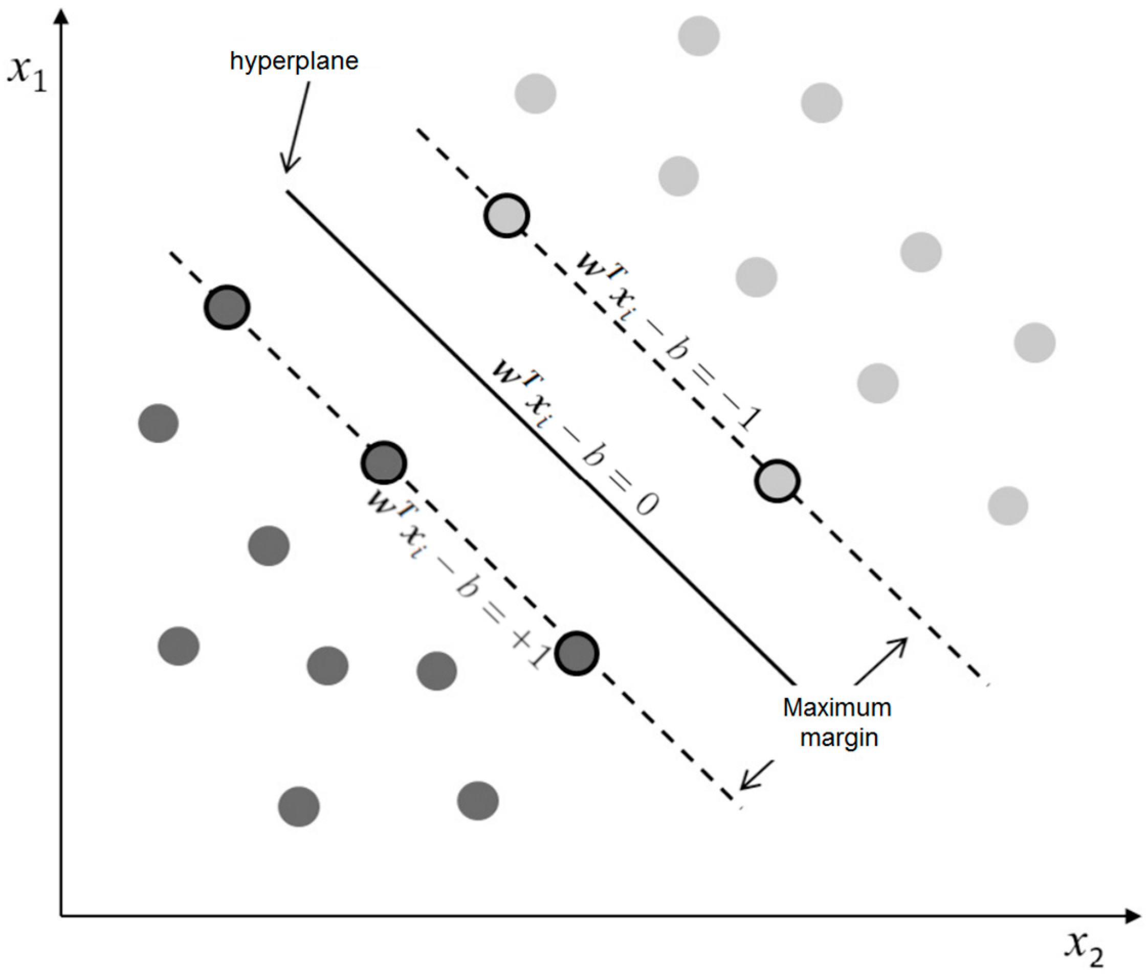
In the linearly separable case, the linear separator (line in two-variable datasets, the plane in three-variable datasets, and a hyperplane in the dataset with more dimensions) is defined as the decision boundary that classifies each data point to the correct class. The position of the separator is defined by the Support Vectors (SV), a small number of data points from the dataset. In
Figure 1, the SV are represented with the pronounced black contour, the margin lines (parallel lines to the optimal separator passing from the SV) are represented by dashed lines, and the separator is represented by a continuous line. The distance between the two margin lines defines the distance between the two classes. The goal of SVM is to find the linear separator that yields the maximum distance between the two classes.
In real-life phenomena, datasets are contaminated with noise and may contain outliers. In order to treat such datasets [
18], introduced non-negative slack variables,
ξi ≥ 0, ∀
i, and a parameter C, describing the desired tolerance to classification errors. The solution to the problem of identifying the optimal separator can be dealt with through the Lagrange relaxation procedure of the following equation:
where
measures the distance of vector
from the separator when classified erroneously, and
α1,
α2, …,
αn are the non-negative Lagrange multipliers.
The hyperplane is then defined as:
where:
where
is the set of the support vector indices.
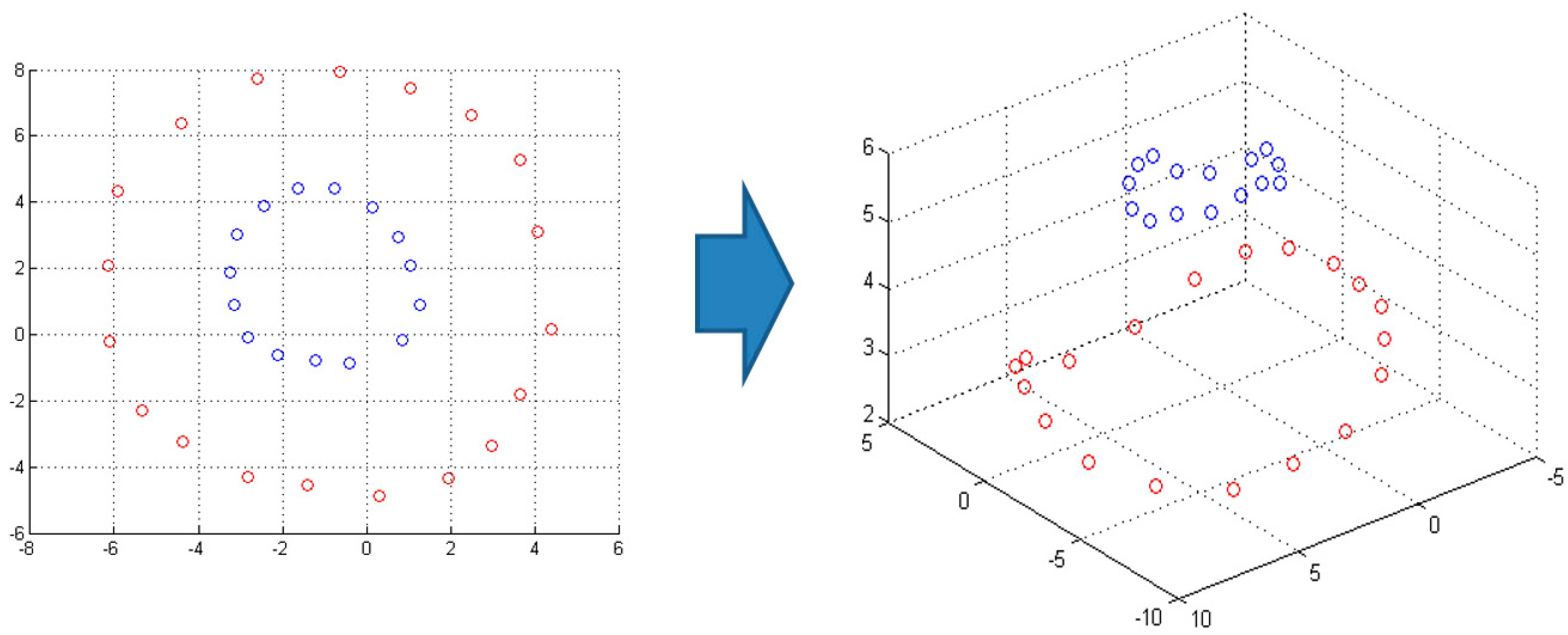
When the dataset is not linearly separable, the SVM model is paired with kernel projection: The initial data space is projected through a kernel function into a higher dimensionality space (called feature space) where the dataset may be linearly separable. In
Figure 2, we depict a dataset that is not linearly separable in the initial two-dimensional data space (left graph), denoted by the red and blue circles. By projecting the dataset in a three-dimensional feature space (right graph) using a kernel function, the linear separation is feasible.
The solution to the dual problem with the projection of Equation (11) now transforms to:
under the constrains
and
where
is the kernel function. The projection to a higher dimensional space, using the kernel trick, is a computationally efficient approach because it projects just the inner product
of the vectors (Our implementation of SVM models is based on LIBSVM [
19]. The software is available at
http://www.csie.ntu.edu.tw/~cjlin/libsvm/).
In this paper, we examine two kernels, the linear kernel and the radial basis function (RBF) kernel. The linear kernel detects the separating hyperplane in the original dimensions of the data space, while the RBF project the initial dataset to a higher dimensional space. The mathematical representation of each kernel is as follows:
The RBF:
where γ is a kernel parameter.
A possible issue when training a model is the problem of overfitting. This is a situation where the selected model is very well fitted to the sample data, but fails to describe the actual true data generating process. In this case, the model’s forecasting ability in out-of-sample data is significantly lower. Thus, an overfitted model provides high accuracy for the in-sample data, while, it fails to reproduce the same performance to the unknown out-of-sample data.
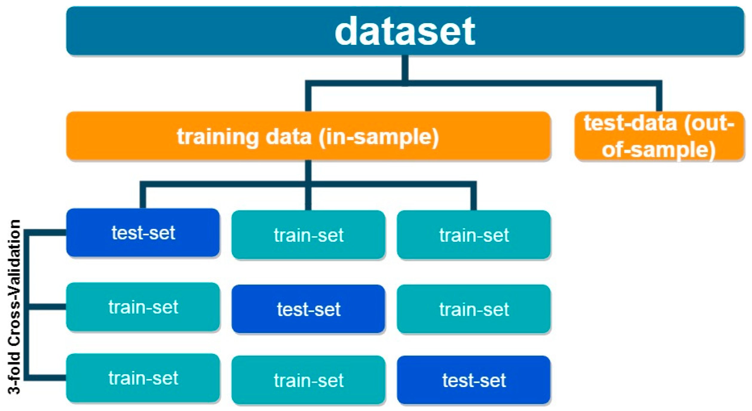
To avoid the problem of overfitting, we implement a
k-fold cross validation procedure. The in-sample data, used for training the model, are divided into
k parts (folds) of equal size. In each iteration, one part is used as the test-set, while the rest are used as the train-set. This process is repeated
k times. Each time a different fold is used for testing and the rest of the folds are used to train the model. The model’s accuracy is evaluated by the average performance over all
k folds for each set of the model’s parameters.
Figure 3 provides a representation of a three-fold cross validation procedure.
In brief, the cross validation is performed to avoid overfitting of our forecasting methodology to the training dataset. The optimal parameters of our forecasting methodology are identified in a coarse-to-fine grid search to avoid exhaustive search, which is computationally enormous to handle [
20]. The SVM methodology finds the optimal linear classificator by maximizing the distance of the marginal data points between the two classes; when the problem is not linearly separable, the kernelization of the system (the projection of the data space into a higher space using a kernel function) allow us to search for non-linear classifiers.
2.2. The Data
The dataset consists of the Eurocoin index and the Simple Sum and Divisia monetary aggregates in three levels of aggregation: M1, M2, and M3. M1 is the sum of currency in circulation and overnight deposits, M2 is the sum of M1, deposits with an agreed maturity of up to two years and deposits redeemable at notice of up to three months and M3 is the sum of M2, repurchase agreements, money market fund shares/units and debt securities with a maturity of up to two years.
The data are monthly covering the period from 2001:1 to 2018:6. The data for the Eurocoin index was obtained from the Centre for Economic Policy Research (CEPR) and the monetary aggregates from Bruegel. Bruegel is a leading independent and non-doctrinal international economics think-tank, contributing to European and global economic policy-making.
The Eurocoin is an index coincident with the euro area business cycle, and among other properties, it is published monthly and includes information on the underlying growth rate of the euro area GDP. It is computed by the Bank of Italy and the CEPR [
21] (the data is available at:
https://eurocoin.cepr.org/). The monetary aggregates used by most central banks are simple-sum indices in which all monetary components are assigned the same weight. The Divisia indices, originated from [
4], apply different weights to different assets in accordance with the degree of their contribution to the flow of monetary services in an economy. The computation of the Divisia monetary aggregates for the Eurozone was conducted by [
22] (the data is available at:
http://bruegel.org/publications/datasets/divisia-monetary-aggregates-for-the-euro-area/).
In what follows, we use the levels of the Eurocoin index, since seasonality and time trend are well removed by the Bank of Italy and CEPR [
21], and log-levels for all the monetary aggregates. We do not use log returns for the monetary aggregates because we would be testing for money super neutrality. According to the money neutrality theory, changes in the money supply only affect nominal variables (exchange rates, wages and prices) and not real variables (GDP, unemployment, etc.), while the super-neutrality theory assumes that changes in the rate of money supply growth do not affect real variables. Moreover, since the SVM methodology is robust in the existence of unit root processes in the data [
23], we did not test for stationarity and proceeded with the levels of all variables. The data are normalized to the [−1,1] range.
We split our 195-samples dataset into two parts: The first 156 observations form the training sample, and the rest 39 observations were used to evaluate the out-of-sample forecasting accuracy (80-20 split). In order to avoid overfitting, we used a 10-fold cross validation and the out-of sample subset that was kept aside during training and which did not participate in the cross validation procedure, was used to evaluate the generalization ability of the model (out-of-sample forecasting). We implemented the linear and the RBF kernels (the parameter c was scanned from 1 to 50.001 with step 100 and g from 1 to 101 with step 10.).
3. Empirical Results
We proceeded in three steps. The first step was to use the SVM to produce the best autoregressive model AR(q) in forecasting the Eurocoin index. The AR(q) model is the simplest model structure where lagged values of the dependent variable are used to forecast the current value and is defined as:
where
X is the Eurocoin index, q the maximum number of lags and
φi the parameter vector of the lags to be estimated.
We used q = 1–15 and tested the corresponding directional accuracy with respect to the Eurocoin index. The best AR model was the one that included six lags for both, linear and RBF kernel; the AR model is not overfitted, since the in-sample and out-of-sample accuracies are high and close (
Figure 4 and
Figure 5). Overall, the best AR model is the one equipped with the RBF kernel with in-sample accuracy of 84.62% and out-of-sample accuracy 79.49%.
In the second step, we built structural directional forecasting models by augmenting the best AR(6) with the monetary aggregates and their lags, and we evaluated their ability to forecast the Eurocoin index.
Finally, we attempt to provide evidence on the issue of money neutrality. We create and test the forecasting accuracy of six structural models by augmenting the best AR models with the inclusion one-by-one of all simple sum and Divisia monetary aggregates. If the augmented model outperforms, in terms of directional forecasting accuracy, the corresponding AR one, then this is interpreted as evidence against money neutrality. Money matters as it is mentioned in the relevant literature. In the opposing case, where the augmented models are unable to outperform the AR ones, we have evidence of money neutrality. The Eurocoin is an index that measures the real GDP growth rate in the euro area. Thus, by providing evidence that it can be forecasted more accurately with the inclusion of the monetary aggregates is interpreted as direct evidence that money affects not only the nominal, but the real economic activity as well. In this context, we can also compare the forecasting ability of the simple sum and the Divisia monetary aggregates. If money is not neutral, then we expect that the Divisia will be superior to the simple sum ones in terms of forecasting ability. The Divisia are constructed in a theoretically “correct” procedure following aggregation theory. The simple sum ones are mere sums of the included assets. These results are presented in
Table 1 for the linear kernel and in
Table 2 for the RBF one.
We can observe from
Table 1 that the inclusion of the monetary aggregates in the structural models improved the in-sample forecasting accuracy of the AR(6) one for all six aggregates. The out-of-sample forecasting accuracy was improved for the simple sum M1, Divisia M1, Divisia M2, and Divisia M3, while it remained the same as the AR model for the simple sum M2 and the simple sum M3. Thus, the augmented models improve the directional forecasting of the Eurocoin index -as they are compared to the AR ones- providing evidence against money neutrality.
In
Table 2, we present the results for the RBF kernel. Augmenting the AR(6) model with the monetary aggregates provides an inferior in-sample forecasting accuracy. More specifically, the AR(6) model coupled with the RBF kernel reaches an accuracy of 84.62%. The maximum accuracy for the monetary aggregates augmented models is achieved with the simple sum M2 and Divisia M2 and is equal to 77.56% for both. The out-of-sample results are qualitatively similar: No monetary aggregate augmented model outperforms the AR(6) model that reaches a 79.49% accuracy. The maximum accuracy for the monetary aggregates augmented models is achieved with the simple sum M3 and Divisia M3 and is equal 74.36% and 64.10% respectively.
Moreover, we observe that in the case of the structural models coupled with the RBF kernel, the in-sample forecasting accuracy is significantly higher than the out-of-sample one. This may be the result of possible overfitting in the training procedure. In this case, the model fits the sample at hand very well, but not the true data generating process. As a result, we achieve a high forecasting accuracy in the sample, but this is significantly reduced when new data are used. Thus, the results in the case of the RBF kernel must be interpreted with caution.
According to the above, the best overall model is the augmented model with the Divisia M2 as the explanatory variable coupled with the linear kernel reaching 82.05% out-of-sample accuracy and 87.18% in-sample accuracy. This finding proves that AR models are less accurate than their respective structural models, and we created a model of Eurocoin directional forecasting with high accuracy.
4. Conclusion
In this study, using the money supply, we attempt to forecast, out-of-sample, the economic activity within the euro area. In this macroeconomic setting, we innovate by employing in the empirical section a machine learning methodology, the support vector machines (SVM) for binary classification. Moreover, instead of using the low frequency (quarterly) GDP time series to measure economic activity, we use the Eurocoin index that is available in monthly frequency from January 2001 to June 2018. The Eurocoin is an index that measures the growth rate of the euro area GDP, and it is produced by the Bank of Italy and the CEPR. Furthermore, we use two alternative sets of monetary aggregates as a proxy for money supply: The commonly used by most statistical agencies and central banks all over the world simple sum monetary aggregates and the theoretically correct, as they are constructed according to the index numbers theory, Divisia monetary aggregates proposed by the Barnett Critique [
5,
6]. Both aggregates are used in three levels of aggregation, from the narrow M1 to the broader M2 and M3 aggregates.
The forecasting methodology employed comes from the area of machine learning and is the support vector machines supervised algorithm for classification. Two alternative kernels are used in the taring process: The linear and radial basis function (RBF). First, we train the best possible Autoregressive Models (AR) to forecast the Eurocoin. Next, we train structural models by adding one-by-one each of the six alternative monetary aggregates (simple sum M1, simple sum M2, simple sum M3, Divisia M1, Divisia M2 and Divisia M3). This empirical setup allows us to derive significant inference in several directions. First, we can compare the forecasting accuracy of the simple sum and the Divisia monetary aggregates in terms of the Eurocoin index (euro area GDP growth rate). Second, in the case that some of the aggregates can adequately forecast economic activity better than the best AR models, this can be interpreted as evidence against money neutrality; money, in that case, would matter for the economy. The money supply at t forecasts economic activity at t + 1. If the structural models (with the use of the monetary aggregates) cannot forecast the Eurocoin index better than the AR models, then we can conclude that money is neutral as it cannot adequately forecast economic activity: The money supply at t cannot forecast the economic activity at t + 1.
The empirical results show that the structural models that use the monetary aggregates (using the linear kernel) outperform the autoregressive ones in terms of forecasting accuracy. In that case, the money supply (expressed by the simple sum and Divisia monetary aggregates) affects the economic activity, thus, since money can forecast economic activity as measured by the Eurocoin index, we provide empirical evidence against money neutrality: Money seems to matter.
Moreover, the Divisia monetary aggregates outperform the relevant, simple sum ones both in-sample and out-of-sample. In one case only (the M1 out-of-sample) the two aggregates have the same accuracy. The best overall out-of-sample forecasting accuracy is achieved with the Divisia M2 monetary aggregate reaching 82.05%. Thus, we conclude that the Divisia monetary aggregates, overall, outperform the simple sum ones in terms of forecasting the Eurocoin index.
The policy implications of these results are obvious for the European Central Bank (ECB) when designing and implementing monetary policy in the euro area. The money supply was abandoned as a target for the monetary policy three decades ago as it did not seem to adhere closely to economic activity. As a result, the monetary aggregates were replaced by the interest rate as a tool for the implementation of monetary policy by most large central banks around the world. Our results corroborate the strand of similar studies that provide evidence that the loose relationship between the money supply and the economic activity was an inherent drawback of the monetary aggregates that were (and still are) used: The simple sum. The theoretically correct Divisia monetary aggregates seem to overcome this problem, and thus, the ECB and other central banks may consider increasing the role of monetary aggregates and more specifically the Divisia ones, alongside with the interest rates, in the designing and implementation of the monetary policy.


