Article

A New Regularized Reconstruction Algorithm Based on Compressed Sensing for the Sparse Underdetermined Problem and Applications of One-Dimensional and Two-Dimensional Signal Recovery

1
School of Computer and Communication Engineering, Northeastern University at Qinhuangdao, Qinhuangdao 066004, China
2
School of Computer Science and Engineering, Northeastern University, Shenyang 110819, China
*
Author to whom correspondence should be addressed.
Algorithms 2019, 12(7), 126; https://doi.org/10.3390/a12070126
Submission received: 27 May 2019 / Revised: 23 June 2019 / Accepted: 24 June 2019 / Published: 26 June 2019
(This article belongs to the Special Issue Data Compression Algorithms and their Applications)

Abstract

:
The compressed sensing theory has been widely used in solving undetermined equations in various fields and has made remarkable achievements. The regularized smooth L0 (ReSL0) reconstruction algorithm adds an error regularization term to the smooth L0(SL0) algorithm, achieving the reconstruction of the signal well in the presence of noise. However, the ReSL0 reconstruction algorithm still has some flaws. It still chooses the original optimization method of SL0 and the Gauss approximation function, but this method has the problem of a sawtooth effect in the later optimization stage, and the convergence effect is not ideal. Therefore, we make two adjustments to the basis of the ReSL0 reconstruction algorithm: firstly, we introduce another CIPF function which has a better approximation effect than Gauss function; secondly, we combine the steepest descent method and Newton method in terms of the algorithm optimization. Then, a novel regularized recovery algorithm named combined regularized smooth L0 (CReSL0) is proposed. Under the same experimental conditions, the CReSL0 algorithm is compared with other popular reconstruction algorithms. Overall, the CReSL0 algorithm achieves excellent reconstruction performance in terms of the peak signal-to-noise ratio (PSNR) and run-time for both a one-dimensional Gauss signal and two-dimensional image reconstruction tasks.

1. Introduction

Compressed sensing, also known as compressive sampling or sparse sampling, is a technique for finding sparse solutions of underdetermined linear systems. In 2006, Donoho et al. proposed the concept of compressed sensing (CS), which provides a new idea for signal sampling theory [1,2,3]. CS theory has attracted the attention of many experts and scholars and has been widely used in many fields such as signal processing [4] , radar imaging [5], wireless sensor networks [6], blind source separation [7] and so on. According to compressed sensing theory, if the signal is sparse on a dictionary basis, it can be sampled and compressed simultaneously with an observation matrix that is not related to the sparse dictionary to project the high-dimensional signal in the low-dimensional space. Then, the sparse representation vector of the signal can be obtained by solving the l 0 norm optimization problem, and the original signal will be reconstructed.
Unlike the traditional Nyquist sampling theory, compressed sensing theory requires that the signal must be compressible or sparse in a transform space. In other words, the new compressed sensing theory breaks through the limitation of the traditional Nyquist sampling theorem in signal acquisition, innovatively realizes the simultaneous sampling and compression of signals, and can accurately recover the original signals by random sampling compared with the traditional method. Accurate signal reconstruction refers to the accurate recovery of the original high-dimensional signal from a small amount of data. The essence of the reconstruction process is to find the optimal solution for a set of undetermined equations. Therefore, it can be seen that the reconstruction algorithm plays an important role in all of compressed sensing theory. The reasonable design and selection of the method is directly related to the accuracy of reconstructed data. The higher the reconstructed accuracy, the greater the practicality of the theory.
Compressed sensing theory, with its unique advantages, has made rapid development and at the same time has also set off a research boom. At present, many universities and research institutes have joined in the research of compressed sensing theory and have achieved many excellent results. Research results for signal reconstruction algorithms for compressed sensing are emerging in an endless stream. There are many kinds of compressed sensing reconstruction algorithms, but the most common variants are greedy and convex relaxation algorithms. Among greedy algorithms, the earliest matching pursuit algorithm used for reconstruction is the matching pursuit algorithm (MP) [8]. Additionally, there are many variants of it, such as the orthogonal matching pursuit algorithm (OMP) [9], subspace pursuit algorithm (SP) [10], compressed sampling matching pursuit algorithm (CoSaMP) [11], sparsity adaptive matching pursuit algorithm (SAMP) [12], multi-orthogonal least squares algorithm (MOLS) [13] and so on. There are also many convex relaxation optimization algorithms, such as the basis pursuit algorithm (BP) [14], interior point algorithm [15], gradient projection for sparse reconstruction algorithm (GPSR) [16], fast iterative threshold shrinkage algorithm (FISTA) [17] and so on.
In 2009, Mohimani proposed a smooth SL0 [18] reconstruction algorithm that directly minimizes the l0 norm. Compared with the previous convex optimization method, in this algorithm, the discrete l0 norm is replaced by the continuous Gaussian function with parameters to construct a new objective function, then the steepest descent method is used to minimize the approximate continuous function, and finally, the minimal solution is projected into the solution space to satisfy the constraints. From the implementation process of the algorithm, the algorithm combines the rapidity of the greedy algorithm and the accuracy of convex optimization and is a better reconstruction algorithm. There are many improved algorithms based on the SL0 algorithm. Recently, in [5], the author proposed a regularized smooth l 0 reconstruction algorithm called ReSL0 [5], which can reconstruct the signal in the presence of noise, and the reconstruction effect is impressive. However, the ReSL0 algorithm uses the Gauss approximation function and the steepest descent optimization method of the SL0 algorithm. On the one hand, through our research and investigation, we find that many approximation functions are better than the Gauss function, such as the approximation function in [19]; on the other hand, although the steepest descent optimization method adopted by ReSL0 does not require the accurate initial value, the optimization algorithm itself has drawbacks. In the early stage of the algorithm, the steepest descent method does have the best approach; however, in the later stage of optimization, there will be a jagged optimization path, and the convergence becomes very slow. The well-known Newton method has second-order convergence, but the Newton method requires a more accurate initial value, and it is not easy to get a perfect initial value. For this reason, we add the combined optimization method of the steepest descent method and Newton method to the ReSL0 algorithm and select the approximation function as used in [19]. Thus, the combined-optimization ReSL0 algorithm is proposed in this paper, which is called the CReSL0 algorithm.

2. Preliminaries

In the theory of compressed sensing, if a signal is sparsely represented under an orthogonal basis ( ψ 1 , ψ 2 , , ψ N ) , the original signal s R N with length N ( N > > M ) can be reconstructed through the sensing matrix A R M N and the observation vector y R M obtained from m instances of observation. Suppose s R N is a real signal and ( ψ 1 , ψ 2 , , ψ N ) is a set of orthogonal vectors, then the signal s can be expressed as s = i = 1 N ψ i x i , where x i is the representation coefficient of the signal s under the corresponding orthogonal basis (i.e., x i = < s , ψ i > , < , > denotes the inner product operation). If the ψ i and x i in the above formulas are expressed in matrix form, respectively, the orthogonal basis matrix Ψ R N N and the representation coefficients vector x R N , s = i = 1 N ψ i x i can be written in the following matrix form,
s = Ψ x
when the coefficients indicate that there are few non-zero elements in vector x ; that is, x is sparse. According to the CS theory described above, we can use the observation matrix Φ to observe m times to get y = Φ s , where y is the observed M-dimensional column vector. According to (1), we can further get y = Φ Ψ x . Let A = Φ Ψ and y = Φ Ψ x be rewritten as y = A x , which is the general expression of compressed sensing, where matrix A is called the sensing matrix. After that, x can be reconstructed from y by sensing matrix A and the observation vectors y . However, in most cases, the observed signal in reality will be contaminated by noise, so a more general form is given here.
y = A x + w
in which w is usually Gauss white noise. Besides, the matrix A needs to satisfy the restricted isometry property (RIP) [3] described below:
( 1 δ k ) | | x | | 2 2 | | A x | | 2 2 ( 1 + δ k ) | | x | | 2 2
Although Equation (2) is an underdetermined equation problem, the signal can be recovered because of the sparsity of the signal by solving an l0 -minimization problem, as below:
min   | | x | | 0      s . t .        | | y A x | | 2 ε

3. ReSL0 Algorithm

The ReSL0 algorithm is an improved algorithm on the basis of the SL0 algorithm. The advantage of the ReSL0 algorithm over the SL0 algorithm is that it can reconstruct the algorithm in the presence of noise. That is to say, Equation (4) will be studied and analyzed. The ReSL0 algorithm only changes the projection part of the SL0 algorithm. The regularization factor and error term are added to adjust the sparse solution and error term, and then a compromise value between the two terms is taken to realize signal reconstruction in the case of noise. The overall structure of the ReSL0 algorithm is the same as that of the SL0 algorithm, which consists of the inner and outer loops. The inner loop is composed of the steepest descent optimization method, as x ^ x + μ σ 2 F σ ( x ) . The outer loop features the following improvements:
min x p | | x p x ^ | | 2      s . t .        | | A x p y | | 2 δ
The Lagrangian form of the above formula is as follows:
x ^ p = arg    min x p | | x p x ^ | | 2 2    +     λ    | | A x p y | | 2 2 ,
where λ is a positive regularization factor, which is used to compromise the sparse solution and reconstruction residual term. Then, Equation (6) can be obtained by the weighted least squares method as follows:
x ^ p = ( I n + λ A H A ) 1 ( x ^ + λ A H y ) ,
where I n is the unit matrix of m m and A H is the conjugated transposed matrix of A . We can see from [18] that
( I n + A B ) 1 = I A ( I n + B A ) 1 B
Then, the following solution is obtained:
x ^ p = x ^ A H ( A A H I n + λ 1 I m ) 1 ( A x ^ y )
Next, the pseudocode of the ReSL0 algorithm can be summarized as Algorithm 1.
Algorithm 1. The pseudo-code of the ReSL0 algorithm.
Initialization:
  (1) Set L   ,   μ > 0 and x ^ 0 = A H ( A A H ) 1 y .
  (2) Set 0 < ρ < 1 , σ 1 , σ J and σ j = ρ σ j 1 where j > 1 .
While σ j > σ J
  (1) Let σ = σ j .
  (2) Initialization: x = x ^ j 1 .
    -for k = 1 , , L
    (a) x x + μ x exp ( x 2 / ( 2 σ 2 ) ) .
    (b) x = x A H ( A A H I n + λ 1 I m ) 1 ( A x y ) .
  (3) Set x ^ j = x .
The estimated value is x ^ = x ^ j .

4. CReSL0 Algorithm

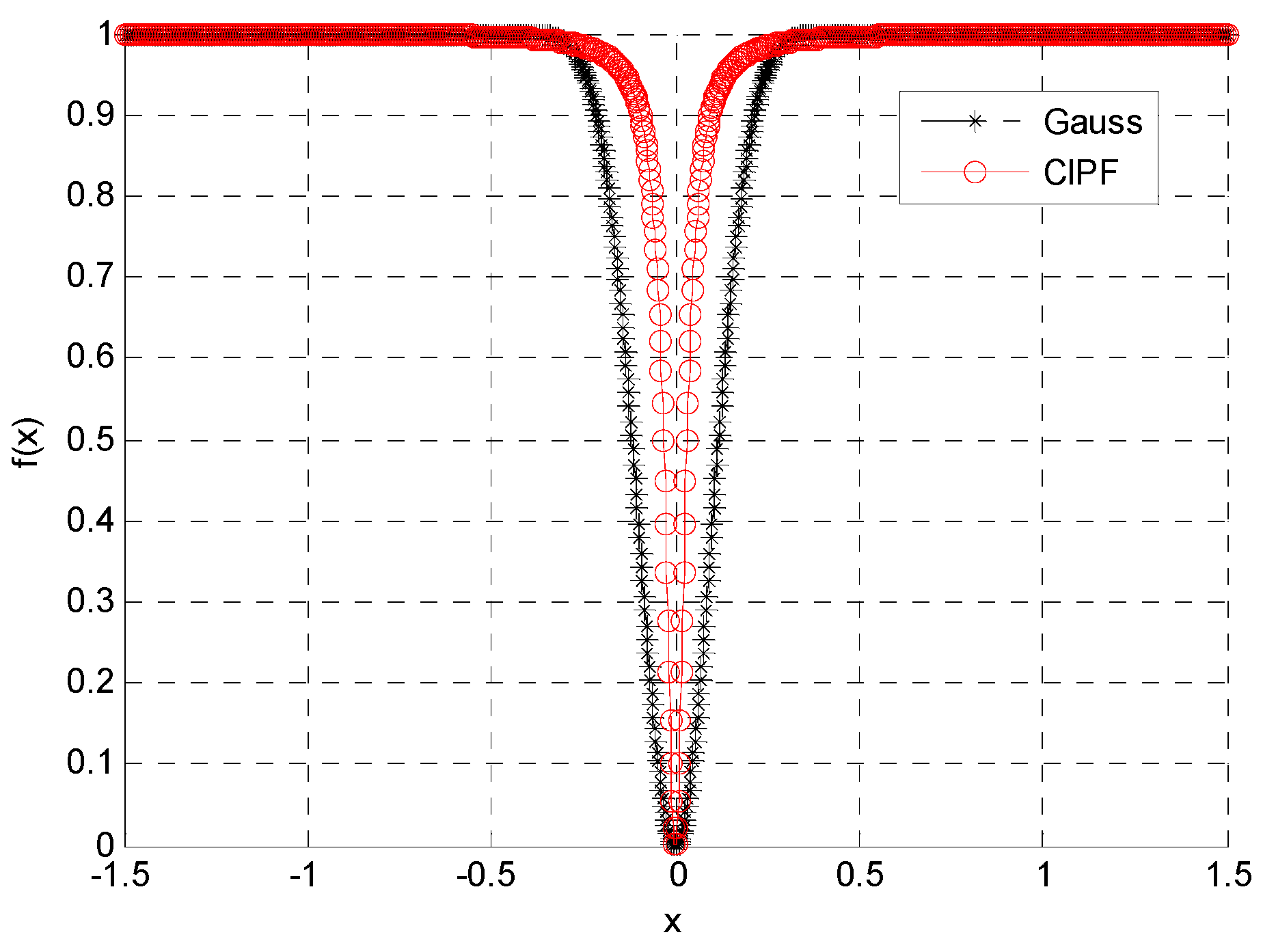
4.1. Selection of Approximation Function

In the section above, it can be clearly seen that the ReSL0 algorithm mainly changes the original projection part of the basis of the SL0 algorithm, but the optimization method still chooses the steepest descent method, and the approximation function is also the Gauss function. In this paper, the CIPF function in [19] will be selected as follows:
f σ ( x ) = 1 σ 2 α x 2 + σ 2 ,
where α = 10 . σ determines the steepness of the function. When σ = 0.01 , the steepness comparison between this function and the Gauss function is shown in Figure 1.
From Figure 1, we can clearly see that the CIPF function is much steeper than the Gauss function when it is approaching zero. When they are very close to zero, the steepness of the two functions is almost the same. From Figure 2, we can easily see that
lim σ 0 f σ ( x i ) = { 1 , x = 0 0 , x 0
Then, the zero norm of the reconstructed signal can be obtained as follows:
| | x | | 0 = lim σ 0 i = 1 N f σ ( x i )
Thus, Equation (4) can then be transformed into the following form:
min    lim σ 0 i = 1 N f σ ( x i )       s . t .         | | y A x | | 2 ε

4.2. Selection of Optimization Method

In this paper, the combination of the steepest descent method and Newton method is used to replace the simple steepest descent method in ReSL0. From Figure 1, we can see that the steepness of the Gauss function and CIPF function is almost the same when they are very close to zero; that is, the final stage of the optimization process. In addition, the form of the Gauss function y σ ( x ) = exp ( x 2 / 2 σ 2 ) will be much simpler. Thus, we select the CIPF function to approximate zero norm in the early steepest descent method part (that is, only the first derivative is needed). We choose the Gauss function to approximate zero norm in the latter Newton method part (that is, the second derivative is needed). Only in this way can we attain a more accurate reconstruction in less time. In the next, let
F σ ( x i ) =     lim σ 0 i = 1 N f σ ( x i )
Y σ ( x i ) =     lim σ 0 i = 1 N y σ ( x i )
Then, the gradients of Equations (14) and (15) are obtained as follows, respectively:
F σ ( x ) = [ f σ ( x 1 ) x 1 , , f σ ( x N ) x N ] T ,
where f σ ( x i ) x i = 2 α σ 2 x i ( α x i 2 + σ 2 ) 2 .
Y σ ( x ) = [ y σ ( x 1 ) x 1 , , y σ ( x N ) x N ] T ,
where y σ ( x i ) x i = s i σ 2 e x i 2 / 2 σ 2 .
Further, we can get the Hessen matrix of Equation (15) as follows:
2 Y σ ( x ) = [ 2 f σ ( x 1 ) x 1 2 0 0 0 2 f σ ( x 2 ) x 2 2 0 0 0 2 f σ ( x N ) x N 2 ]
where 2 f σ ( x i ) x i 2 = e s i 2 / 2 σ 2 ( σ 2 s i 2 σ 4 ) . From the above Hessen matrix, we see that it cannot be guaranteed that all the elements of the diagonal elements are greater than 0. If the Hessen matrix is not more than 0, it cannot be guaranteed that the direction of the Newton method is always the direction approaching the optimal solution. Thus, we need to further modify the Hessen matrix to get a modified Newton direction to meet the requirement of the positive definite matrix. The modified method replaces the Hessen matrix with the following matrix:
G = 2 Y σ ( x ) + p i I
where the modified factor chosen in this paper is p i = e s i 2 / 2 σ 2 2 s i 2 σ 4 .
In this way, we can get the optimization iteration formulas of the front and back parts of the optimization. The optimization iteration part of the steepest descent method in this paper is as follows:
x x + μ F σ ( x )
The optimization iteration part of the Newton method in this paper is as follows:
x x G 1 Δ Y σ ( x )
In summary, we can get the pseudocode of the CReSL0 algorithm as shown in Algorithm 2.
Algorithm 2. The pseudocode of CReSL0 algorithm.
Initialization:
  (1) Set L ,   μ > 0 and x ^ 0 = A H ( A A H ) 1 y .
  (2) Set σ 1 , , , , , σ J .
While σ j > σ J
  (1) Let σ = σ j .
  (2) Initialization: x = x ^ j 1 .
    -for k = 1 , , β , , L
    If k β (a) x x + μ F σ ( x ) .
        (b) x x A H ( A A H I n + λ 1 I m ) 1 ( A x y ) .
    Else  (c) x x G 1 Δ Y σ ( x ) .
        (d) x x A H ( A A H I n + λ 1 I m ) 1 ( A x y ) .
  (3) Set x ^ j = x .
The estimated value is x ^ = x ^ j .

4.3. Selection of Parameters

For the selection of μ , from Algorithm 2, we can obtain the steepest descent method part x x + μ F σ ( x ) of the CReSL0 algorithm; that is, x x + μ 2 α σ 2 x i / ( α x i 2 + σ 2 ) 2 . According to Equation (11), we know that x x + μ 2 α σ 2 x i / ( α x i 2 + σ 2 ) 2 must be approaching zero when σ 0 , so we can obtain μ = σ 2 / 2 α . For the selection of the σ generation mode, we do not utilize ρ ( 0 < ρ < 1 ) times the decreasing mode, but select the generation mode σ t = σ 1 exp ( log ( σ 1 / σ T ) ( t 1 ) / ( T 1 ) )   for t = 1 , 2 , , T in [15].

5. Simulation and Results

In order to verify the performance of the proposed algorithm, we compare the popular WReSL0 [19] and ReSL0 [5] algorithms with the proposed CReSL0 algorithm in reconstructing a one-dimensional signal and two-dimensional image by the MATLAB simulation platform. The MATLAB simulation platform runs on a 64-bit Intel i5-4210 [email protected] processor and Windows 8 system. The noise added in each experiment is Gauss white noise, which is generated by i N ( 0 , 1 ) . i in all the following experiments is set as 0.01. The peak reconstruction signal-to-noise ratio (PSNR) and running time of the reconstruction algorithms are selected as the performance indicators. The running time is obtained by the tic and toc functions of MATLAB. The PSNR of the one-dimensional signal and two-dimensional signal is defined by the following two formulas, respectively:
P S N R = 20 log ( n o r m ( x ) / n o r m ( x x ^ ) )
P S N R = 10 log ( 255 2 m n / i j ( x ^ ( i , j ) x ( i , j ) ) )
Each algorithm chooses the parameter settings when its performance is the best. For WReSL0, the iteration time T = 30 , step length L = 5 , and regularization parameter λ = 0.1 ; for ReSL0, the iteration step L = 5 , constant μ = 2.5 , regular parameter λ = 1.5 ; for CReSL0, the iteration time T = 30 , step length L = 5 , constant μ = 2.5 , regular parameter λ = 1.5 , β = 3 . σ J = 0.01 is set for all algorithms.

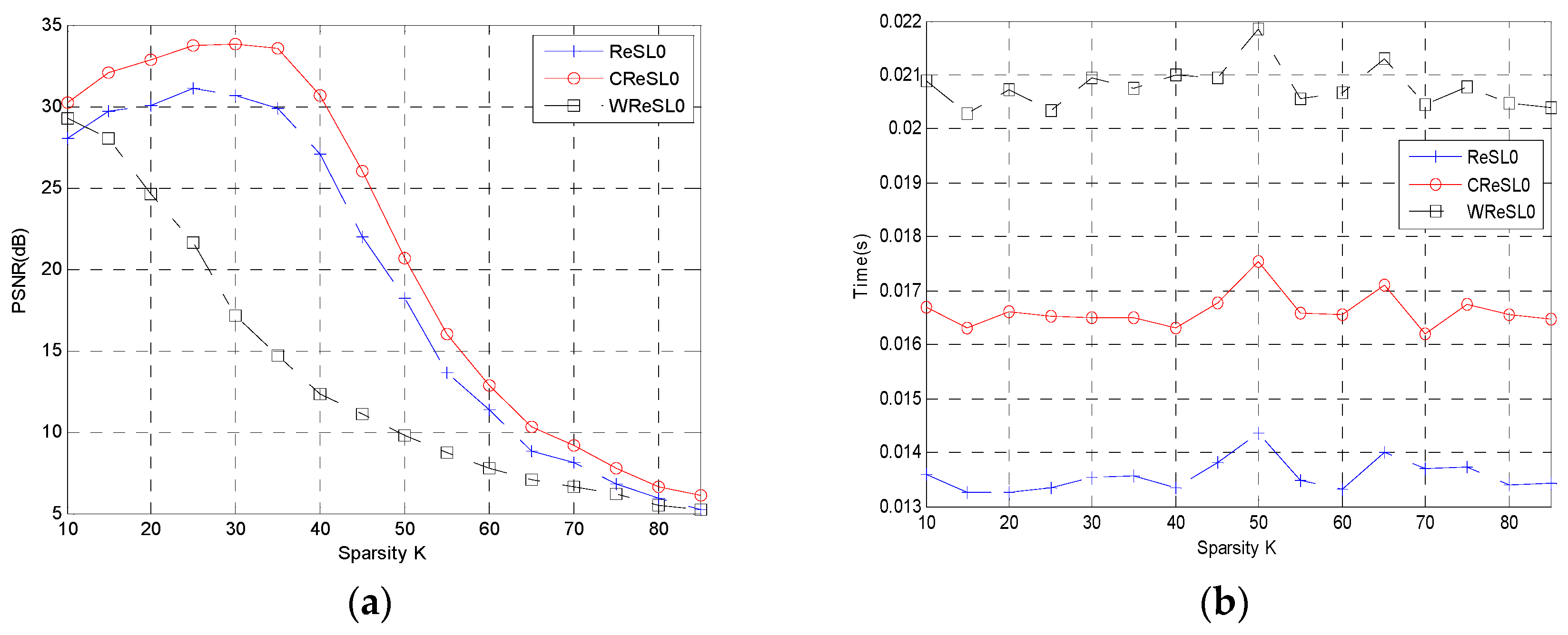
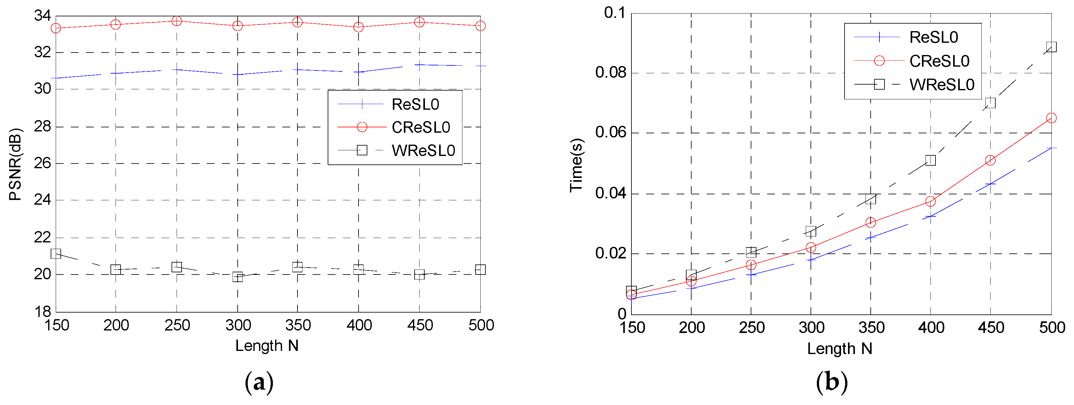
5.1. Reconstruction of One-Dimensional Gauss Signal

Firstly, the one-dimensional Gauss signal is chosen as the signal to be reconstructed, and the Gauss random matrix is used as the measurement matrix. The aim of this experiment is to set the signal length to 256 and the measurement number to 128 to study the reconstruction performance of each algorithm for different sparsities in the presence of noise. For each sparsity value (15–85, where the interval is 5), we repeat the process 100 times and take the final average PSNR as the final PSNR. The final experimental PSNR values are shown in Figure 2a, and the average reconstruction time of the corresponding algorithms is shown in Figure 2b.
As shown clearly in Figure 2a, the PSNR of CReSL0 algorithm is much higher than that of the other two algorithms for each sparsity value. Especially when the sparsity is 30, the PSNR of the CReSL0 algorithm proposed in this paper can reach 34, while the other two algorithms can only get to 31 and 18, respectively. From Figure 2b, the least time-consuming reconstruction algorithm is the ReSL0 algorithm, but the proposed CReSL0 algorithm still takes less time than the WReSL0 algorithm. Additionally, the reconstruction time of the three algorithms is not very different.
Secondly, the reconstruction performance of different signal lengths (150–500, where the interval is 50) is studied in the presence of noise. The reconstruction signal still chooses the one-dimensional Gauss signal. For each signal length, the measured value and sparsity are one-half and one-tenth of the signal length, respectively. Each experiment will also measure 100 times, and the final average PSNR will be taken as the final PSNR. The final experimental PSNR values are shown in Figure 3a, and the average reconstruction times of the corresponding algorithms are shown in Figure 3b.
As can be seen clearly from Figure 3a, the reconstruction PSNR of the three algorithms for different length signals tends to be stable. This shows that the reconstructed PSNR of these three algorithms is basically not affected by the length, and the PSNR of CReSL0 algorithm is still the highest for the reconstructed signals with different lengths. In Figure 3b, we see that the reconstruction time of these three algorithms increases with different length signals. However, the reconstruction time of the WReSL0 algorithm increases the fastest, followed by the CReSL0 algorithm and ReSL0 algorithm.

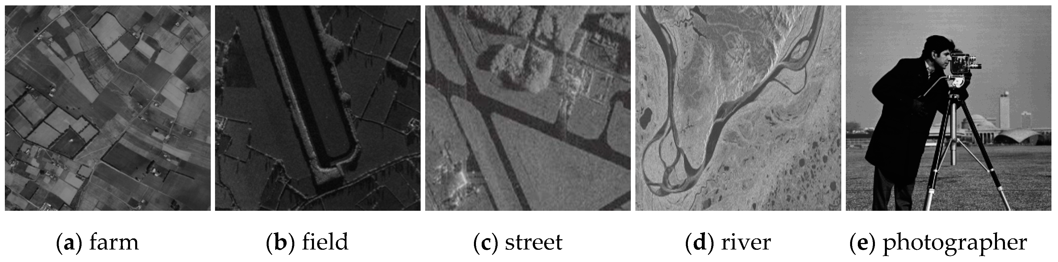
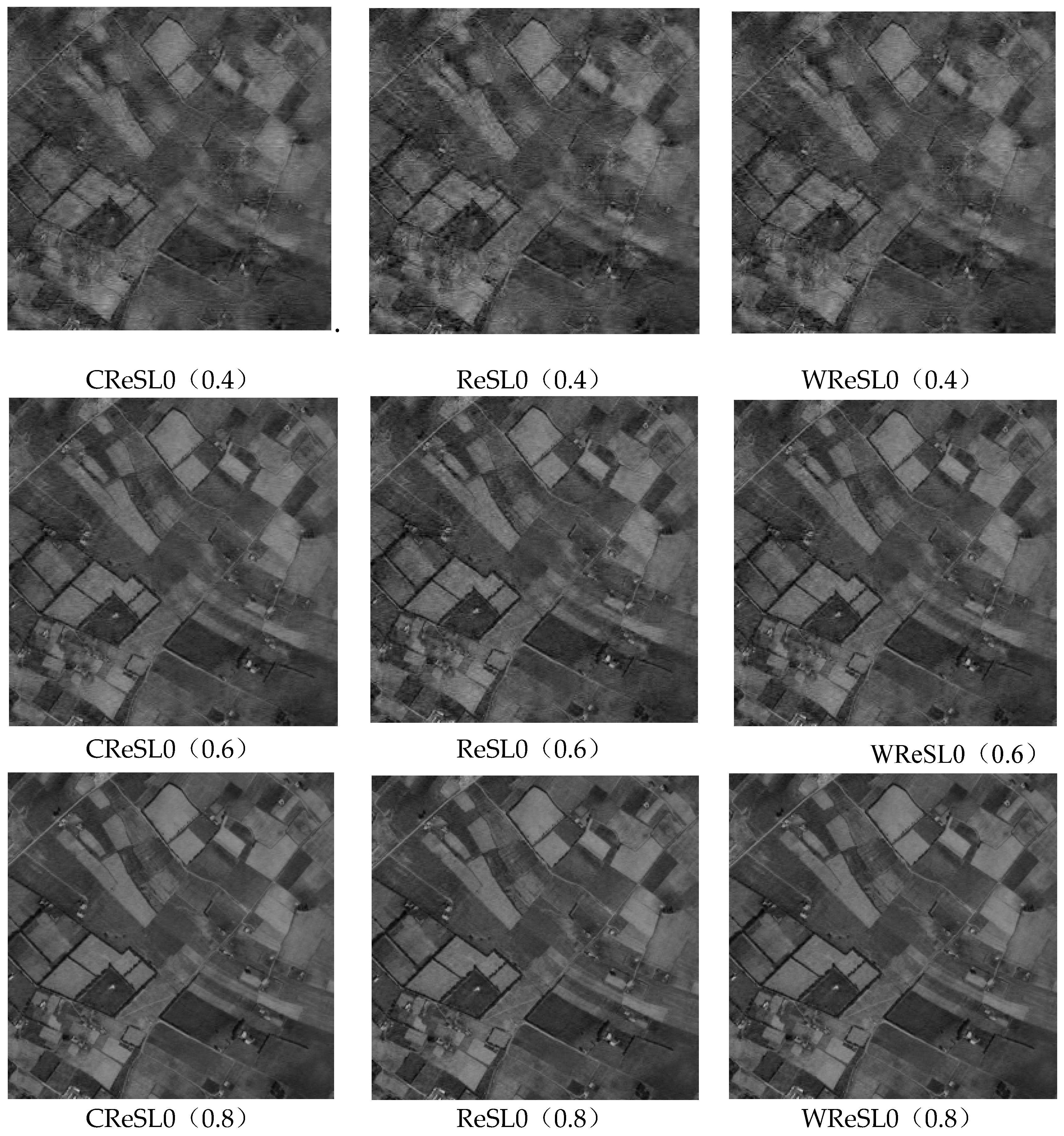
5.2. Reconstruction of Two-Dimensional Image Signal

Since the image itself is not sparse, the discrete wavelet transform (DWT) basis is selected as Ψ in Equation (1) to sparse the image. In addition, the image is a two-dimensional signal, which needs to be undersampled from two dimensions. Thus, Equation (1) is termed as below for the image reconstruction:
x = D W T s i m a g e D W T H
where D W T H is the conjugated transposed matrix of D W T . Next, the two-dimensional reconstruction of the image here treats each column of the image as a one-dimensional signal and then carries out further image reconstruction.
Firstly, five images in Figure 4 are selected as experimental reconstructed images. The dimension of the images is 256*256. The selected measurement matrix is still the Gauss random matrix, and the dimension of the measurement matrix is 190*256. The reconstructed PSNR of each algorithm and the running time are shown in Table 1.
From Table 1, it can be clearly seen that the PSNR of the CReSL0 algorithm is superior to the PSNR obtained by the other two algorithms for all different reconstructed images. CReSL0 takes more time than the ReSL0 algorithm, but less time than the WReSL0 algorithm. For different images, the PSNR obtained by each algorithm and the running time of each algorithm vary slightly, and the overall change is not significant. Therefore, the reconstruction performance of each algorithm is very stable. The ratio of PSNR and time is included, and the ratio of PSNR and the time of the CReSL0 algorithm is smaller than that of ReSL0 but bigger than that of WReSL0.
Secondly, the experiment chooses the image in Figure 4a to study the reconstruction effect of each algorithm under different compression ratios (the ratio of measured value to signal length). The compression ratios are set as 0.4, 0.6 and 0.8, respectively. The recovery images are shown in Figure 5. The reconstruction PSNR and the running time of each algorithm are shown in Table 2.
As shown in Figure 5, with the increment of the compression ratio, the reconstruction effect of each algorithm improves. Visually, we cannot judge which algorithm has the better reconstruction effect. However, from the data in Table 2, we can clearly see that the PNSR of the CReSL0 algorithm proposed in this paper is the highest for each compression ratio. The reconstruction of the CReSL0 algorithm takes a little more time than that of the ReSL0 algorithm but a little less time than that of the WReSL0 algorithm. The ratio of PSNR and time is included, and the ratio of PSNR and time of the CReSL0 algorithm is smaller than that of ReSL0 but bigger than that of WReSL0. Generally speaking, the performance of the algorithm proposed in this paper is the best.

6. Conclusions

This paper makes improvements on the shortcomings of the ReSL0 algorithm. Firstly, after the CIPF approximation function is introduced, the combined approximation model of the Gauss function and CIPF function is proposed, which reduces the run-time of the algorithm to a certain extent compared with the single CIPF approximation model. Then, the optimization objective equation is established. Furthermore, after combining the advantages of the steepest descent method, which does not require the accurate initial value, and the second-order convergence of the Newton method, a combined optimization method is added, which greatly improves the reconstruction performance of the algorithm. Then, the CReSL0 algorithm is proposed. The whole paper introduces the basic theory of compressed sensing and the basic content of the ReSL0 algorithm, and then introduces the CReSL0 algorithm proposed in this paper and makes a detailed analysis and explanation of it. Compared with several popular algorithms, the CReSL0 algorithm proposed in this paper has achieved excellent results with regard to the PSNR and running time, in both one-dimensional Gauss signal reconstruction and two-dimensional image reconstruction.

Author Contributions

Conceptualization, B.W.; Data curation, B.W.; Formal analysis, L.W.; Funding acquisition, B.W.; Investigation, B.W.; Methodology, H.Y.; Project administration, B.W.; Resources, B.W.; Software, L.W.; Supervision, B.W.; Validation, B.W.; Visualization, L.W.; Writing—original draft, B.W. and L.W.; Writing—review & editing, F.X.

Funding

This research was funded by the Natural Science Foundation of Hebei Province (No. F2018501051).

Conflicts of Interest

The authors declare no conflict of interest.

References

  1. Candés, E. Compressive sampling. In Proceedings of the international congress of mathematicians, Madrid, Spain, 22–30 August 2006; pp. 1433–1452. [Google Scholar]
  2. Baraniuk, R. Compressive sensing. IEEE Signal Process. Mag. 2007, 24, 118–121. [Google Scholar] [CrossRef]
  3. Candès, E.; Romberg, J.; Tao, T. Stable signal recovery from incomplete and inaccurate measurements. Commun. Pure Appl. Math. 2006, 59, 1207–1223. [Google Scholar] [CrossRef] [Green Version]
  4. Wang, H.; Guo, Q.; Zhang, G.X.; Li, G.X.; Xiang, W. Thresholded smoothed ℓ° norm for accelerated Sparse recovery. IEEE Commun, Lett. 2015, 19, 953–956. [Google Scholar] [CrossRef]
  5. Bu, H.X.; Tao, R.; Bai, X.; Zhao, J. Regularized smoothed ℓ° norm algorithm and its application to CS-based radar imaging. Signal Process. 2016, 122, 115–122. [Google Scholar] [CrossRef]
  6. Goyal, P.; Singh, B. Subspace pursuit for sparse signal reconstruction in wireless sensor networks. Procedia. Comput. Sci. 2018, 125, 228–233. [Google Scholar] [CrossRef]
  7. Wei-Hong, F.U.; Ai-Li, L.I.; Li-Fen, M.A.; Huang, K.; Yan, X. Underdetermined blind separation based on potential function with estimated parameter’s decreasing sequence. Syst. Eng. Electron. 2014, 36, 619–623. [Google Scholar]
  8. Mallat, S.; Zhang, Z. Matching pursuit in time–frequency dictionary. IEEE Trans. Signal Process. 1993, 41, 3397–3415. [Google Scholar] [CrossRef]
  9. Pati, Y.C.; Rezaiifar, R.; Krishnaprasad, P.S. Orthogonal matching pursuit: Recursive function approximation with applications to wavelet decomposition. In Proceedings of the 27th Asilomar Conference on Signals, Systems and Computers, Pacific Grove, CA, USA, 1–3 November 1993; pp. 40–44. [Google Scholar]
  10. Dai, W.; Milenkovic, O. Subspace pursuit for compressive sensing signal reconstruction. IEEE Trans. Inf. Theory 2009, 5, 2230–2249. [Google Scholar] [CrossRef]
  11. Needell, D.; Tropp, J.A. CoSaMP: Iterative signal recovery from incomplete and inaccurate samples. Commun. ACM 2010, 12, 93–100. [Google Scholar] [CrossRef]
  12. Do, T.T.; Lu, G.; Nguyen, N.; Tran, T.D. Sparsity adaptive matching pursuit algorithm for practical compressed sensing. In Proceedings of the 2008 42nd Asilomar Conference on Signals, Systems and Computers, Pacific Grove, CA, USA, 26–29 October 2008; pp. 581–587. [Google Scholar]
  13. Wang, J.; Li, P. Recovery of Sparse Signals Using Multiple Orthogonal Least Squares. IEEE Trans. Signal Process. 2017, 65, 2049–2061. [Google Scholar] [CrossRef]
  14. Ekanadham, C.; Tranchina, D.; Simoncelli, E.P. Recovery of Sparse Translation-Invariant Signals with Continuous Basis Pursuit. IEEE Trans. Signal Process. 2011, 10, 4735–4744. [Google Scholar] [CrossRef]
  15. Pant, J.K.; Lu, W.S.; Antoniou, A. New Improved Algorithms for Compressive Sensing Based on lp Norm. IEEE Trans. Circuits Syst. II Express Briefs 2014, 61, 198–202. [Google Scholar] [CrossRef]
  16. Figueiredo, M.A.T.; Nowak, R.D.; Wright, S.J. Gradient Projection for Sparse Reconstruction: Application to Compressed Sensing and Other Inverse Problems. IEEE J. Sel. Top. Signal Process 2008, 1, 586–597. [Google Scholar] [CrossRef]
  17. Kim, D.; Fessler, J.A. Another look at the fast iterative shrinkage/thresholding algorithm (FISTA). Siam J. Optim 2018, 28, 223–250. [Google Scholar] [CrossRef]
  18. Mohimani, G.H.; Babaie-Zadeh, M.; Jutten, C. Fast sparse representation based on smoothed ℓ0 norm, in: Independent Component Analysis and Signal Separation. In Proceedings of the International Conference on Latent Variable Analysis and Signal Separation, London, UK, 9–12 September 2007; pp. 389–396. [Google Scholar]
  19. Wang, L.; Yin, X.; Yue, H.; Xiang, J. A regularized weighted smoothed L0 norm minimization method for underdetermined blind source separation. Sensors 2018, 18, 4260. [Google Scholar] [CrossRef] [PubMed]
Figure 1. Comparison of CIPF and Gauss functions.
Algorithms 12 00126 g001
Figure 2. (a) Peak reconstruction signal-to-noise ratio (PSNR) values of each algorithm for different sparsities; (b) running time of each algorithm for different sparsities.
Algorithms 12 00126 g002
Figure 3. (a) PSNR of each algorithm for different signal lengths; (b) running time of each algorithm for different signal lengths.
Algorithms 12 00126 g003
Figure 4. Selected reconstruction images.
Algorithms 12 00126 g004
Figure 5. Reconstructed images of each algorithm for different compression ratios.
Algorithms 12 00126 g005
Table 1. The PSNR, time and PSNR/time of each algorithm for five images. ReSL0: regularized smooth L0; CReSL0: combined regularized smooth L0; WReSL0: weighted regularized smooth L0.
Figure 4PSNR (dB)Time (s)PSNR/Time
CReSL0ReSL0WReSL0CReSL0ReSL0WReSL0CReSL0ReSL0WReSL0
a35.6434.3634.946.565.657.165.436.084.88
b37.0135.3736.016.585.587.185.626.345.02
c36.8235.7836.316.395.607.375.766.394.93
d33.3931.8832.496.485.777.255.155.534.48
e33.0332.0132.686.545.747.185.055.584.55
Table 2. The PSNR, time and PSNR/time of each algorithm for different compression ratios.
CRPSNR (dB)Time (s)PSNR/Time
CReSL0ReSL0WReSL0CReSL0ReSL0WReSL0CReSL0ReSL0WReSL0
0.427.5526.8527.233.232.714.458.539.916.12
0.632.0430.8231.424.754.115.856.757.505.37
0.837.6836.3036.947.506.548.185.025.554.52

